Dirac-Harper Theory for One Dimensional Moiré SuperlatticesPreprint: DHpaper
Abstract
We study a Dirac Harper model for moiré bilayer superlattices where layer antisymmetric strain periodically modulates the interlayer coupling between two honeycomb lattices in one spatial dimension. Discrete and continuum formulations of this model are analyzed. For sufficiently long moiré period the we find low energy spectra that host a manifold of weakly dispersive bands arising from a hierarchy of momentum and position dependent mass inversions. We analyze their charge distributions, mode count and valley-coherence using exact symmetries of the lattice model and approximate symmetries of a four-flavor version of the Jackiw-Rebbi one dimensional solution.
Lattices with competing periodicities are interesting as discrete systems poised in between primitive crystals and random networks Simon82; Ostlund84. When the ratio of the competing periods is a rational fraction , the system is a crystal, although with superlattice translations that are inflated by the divisor . For these systems a spectral analysis of propagating Bloch waves is always possible, but it is ineffective if is large. Famously, the related problem in two dimensions has risen to prominence in addressing the behavior of moiré superlattices in bilayer graphene and twisted stacks of other two dimensional materials Bistritzer; KangVafek; KoshinoTBLG; Po; Song. In these situations, competing periodicities are introduced by a slight rotational misalignment between neighboring layers. For twisted bilayer graphene, important physics occurs near charge neutrality for rotation angles where as a practical necessity, one frequently adopts a continuum description Bistritzer. This is a first-order-in-derivatives expansion about the microscopic Brillouin zone corners, where the microscopic lattice structure appears only through a spatial modulation of matrix-valued coupling between the Dirac operators of individual layers. The correct interpretation of the narrow bands at small twist angles in these models, as well as the analytic structure of its moiré-Bloch bands at general angles, remains the subject of a vigorous discussion KangVafek; KoshinoTBLG; Po; Song.
In this Letter we analyze the one dimensional lattice variant of the twisted bilayer problem using graphene as the prototype. The models we construct are one-dimensional in the sense that they have layer-antisymmetric strains which produce moiré-scale modulation in only one spatial dimension, retaining lattice-scale periodicity in the orthogonal coordinate. With a conserved crystal momentum, the problem takes a strictly one dimensional form whose superlattice period is tuned by the lattice strain. This model generalizes the Harper equation Harper for a scalar field in a one dimensional potential with period
| (1) |
by promoting to a four-component spinor and the coupling parameters to matrices and . We find that this modified Dirac-Harper (DH) model hosts narrow band physics near charge neutrality for sufficiently large moiré periods without fine tuning to a magic angle condition as is required in two dimensions. The near-zero mode structure originates from a reconstruction of the low energy spectrum through a hierarchy of mass inversions necessitated by the matrix structure of the interlayer potential, reminiscent of the multi-flavor variant of the Jackiw Rebbi modelWen. Importantly, unlike its continuum counterpart, the DH model is formulated on a lattice and properly treats the coexistence of the discrete lattice and the moiré periods. The DH model does not admit a sharp identification of a conserved valley degree of freedom. Instead spectral degeneracies and topological properties of the bands are identified through the action of unitary and antinunitary symmetries on the discrete lattice Hamiltonian. Indeed we find that valley degeneracy, presumed to exist in continuum models, is generically preempted by an ordering field that is required by the lattice symmetry and is essential for understanding responses that are activated by the chirality of a bilayer.
One-dimensional bilayer moiré patterns evolving from fully eclipsed () through both staggered (, ) stacking configurations are produced by layer antisymmetric strains (Figure 1a). Two limiting cases are the armchair setting (AC, top) with shear strain and the zigzag setting (ZZ, bottom) with uniaxial strain. The lattice orientations control the projection of the microscopic and points onto the long axis of the folded moiré Brillouin zone, aligning them for AC and keeping them maximally separated in ZZ (Figure 1b). Most of our analysis uses periodic boundary conditions on a large single moiré supercell, restricting .
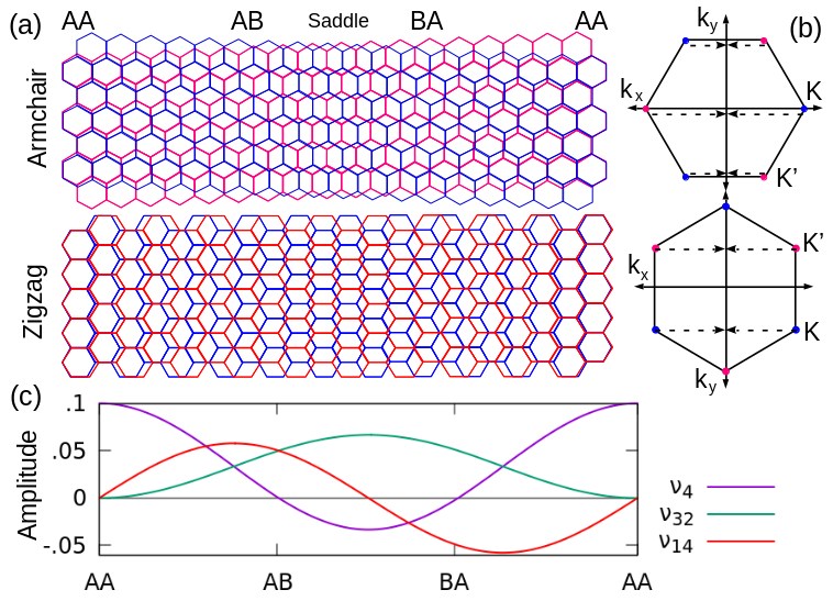
The Harper model for bilayer graphene generalizes Eqn.1
| (2) |
where are four component fields with the conventional ordering of amplitudes on two sublattices and two layers: . Here are block diagonal matrices derived from the nearest neighbor tight-binding kinetic energy for the individual graphene layers supplement and is a spatially modulated interlayer coupling. Defining the Pauli matrices and acting on sublattice index and layer index respectively, the products and form a basis for
where is the hopping amplitude. Explicit formulae for the coefficients and are tabulated in the supplementary section, supplement.
The interlayer coupling is represented as a Fourier interpolation between , , and stacking supplement. The high-symmetry configurations admit a represention in terms of Dirac matrices , , and
where is the interlayer hopping strength. The matrix-valued Fourier coefficients are defined on this basis of mass matrices, allowing the interlayer coupling to be written with amplitudes
plotted in Figure 1c. The and terms ( term) are symmetric (antisymmetric) under , sublattice exchange, and layer exchange. The or -directed choice of sublattice orientation assigns symmetries of to the mirrors , for ZZ and the two-fold rotations , , for AC.
Linearizing this problem in the low energy regime gives the continuum variant of the DH model:
| (3) |
where expresses the expansion of in small about either Dirac point where . This expansion is parameterized by a Fermi velocity where is the microscopic lattice constant. The reduce to for AC and for ZZ supplement. The continuum model requires a choice of valley ( or ) about which to carry out the expansion, and consequently it implies a spectral doubling associated with the conserved valley index. Although this simplification enforces a valley polarization which is not present in the discrete Dirac-Harper model, it can be useful for analytic purposes.
The electronic spectrum of a one-dimensional moiré superlattice in bilayer graphene has been studied previously within a valley-projected continuum theory sanJose1 and in a lattice model Gonzalez which focused on the non-Abelian character of the interlayer coupling matrices. For sufficiently large moiré periods both models predict a manifold of narrow bands near charge neutrality but interestingly they have quite different underlying mode structures Gonzalez. This can be appreciated by comparing the spectra calculated from the discrete DH model (Equation 2) shown in Figure 3. The differences arise from the commutation relations among the mass terms and the kinetic energy operators, represented in Figure 2a as a graph with two edge types. The AC and ZZ structures are distinguished by the relative roles of kinetic energy operators and carrying different commutation relations with the mass terms. These distinctions encode the different symmetries of these structures and persist even in the limit of large moiré period where they control the low energy narrow band physics.

The sublattice-diagonal mass term commutes with both kinetic terms and displaces the layer-degenerate Dirac cones (Figure 2b) by energy (Figure 2c). These displaced cones intersect on a ring at of radius (henceforth called the critical ring) which defines the extent of a band-inverted region. In the full moiré these widths are defined by the extrema in both the and regions, and the spectra in Figure 3 display projections of cones displaced on both scales. The sublattice antisymmetric mass term carries a different commutation relation with each kinetic term, distinguishing the two lattice orientations. Anticommutation with both and opens a gap around zero energy, but commutation with enforces a pair of gap closures on the axis (Figure 2d) supplement. These closures both project to in ZZ of the full moiré, whereas for AC they are maximally separated on either side of the gap (Figure 3). The third mass matrix plays a secondary role: it commutes with every term except , displacing the two cones in opposite directions along the axis (Figure 2. This is reflected in the translation of displaced cones in the ZZ spectrum (Figure 3).

In the gaps opened by we observe a manifold of weakly dispersive bands near zero energy. Although the cones overlap this gap significantly in ZZ, they can be shifted in energy by tuning . For ZZ, pairs of nearly degenerate modes remain weakly dispersive over half the critical ring width and disperse with opposite velocities at the ring edges. Two sets of these together span the full critical ring, and summing over the two inequivalent valleys we find a total of eight modes with charge densities confined to the region (Figure 4). In the case the AC moiré, pairs of nearly degenerate modes span the entire critical ring diameter and are exactly pairwise degenerate. Two of these pairs (four branches) have charge densities peaked in the region, and another two (four branches) have densities that shift from the and regions toward the region as a function of (Figure 4). The total mode count is again eight branches, though with twice the measure of the ZZ modes.

Exact symmetries of the two-valley discrete DH model can be utilized to study valley coherence. Augmenting the symmetries to preserve momentum, these are , trivially , and their product for ZZ and , , and their product for AC supplement. The symmetry of AC is notable because it exchanges valleys and thereby imposes a valley-mixed eigenbasis. It does not commute with the coexisting antiunitary symmetries, enforcing twofold degeneracies. From symmetry under valley exchange in , we can understand the multiplicity to be a consequence of valley coherence. ZZ does not support this type of degeneracy with just one unique nontrivial symmetry operation, but we understand the analogous doubling of the energy eigenstates states to arise from its two momentum-separated valleys.
Low-energy approximate symmetries of the continuum DH model describe single-valley contributions to the mode count. Defining a single-valley ‘time-reversal’ to reverse momenta about a Dirac point, the operator negates the spectrum in a single-valley ‘particle-hole’ symmetry. In AC, leaves the spectrum invariant due to the purely-imaginary kinetic terms, so the spectrum also exhibits chiral symmetry. In ZZ, the purely real kinetic energy terms produce a modified spectrum under , breaking chiral symmetry. Since the weakly-dispersing bands are not exactly at zero energy, this chiral symmetry doubles the mode count in AC, and particle-hole symmetry is consistent with the two sets of half ring-width bands found in ZZ. More precisely, the spectra at are related by the operator , which by commuting with all terms but , preserves the energies while reversing . In AC this manifests in the low bands extending across the full width of the ring, and in ZZ it causes a low-energy approximate degeneracy of states at momenta on the critical ring. Conversely, the sublattice-even is reversed via which also inverts the spectrum. This causes pairs of states at in AC and in ZZ to lie at opposite energies, completing a measure of two full-width bands per valley.
The symmetries of the continuum DH model can be associated with an Altland Zirnbauer symmetry classification. From the local Hamiltonian , one can classify band manifolds by topological invariants computed at each value of . The ZZ Hamiltonian is a real operator which commutes with the complex conjugation operator and therefore lies in class AI. AC commutes with and anticommutes with , putting it into to class BDI. At fixed momentum , these one dimensional Hamiltonians depend on a single position-like coordinate , so the bands of both structures are classified by a topological index Chiu. In AC, the even multiplicity of states in isolated bands prevents juxtaposition of topologically distinct regions. In ZZ, a loop integral of the connection over the moiré period in yields values inside and outside the ring boundary supplement. These two sectors are isolated by the low energy modes that become strongly dispersive at the critical ring.
This analysis identifies the relation between the peaked states found in both settings, but there exists a second set of four peaked states in AC which have no analog in ZZ. The presence of spatially localized modes near zero energy suggest a Jackiw-Rebbi (JR) mechanism for a relativistic model with mass inversion JackiwRebbi. Indeed the regions correspond to sign changes of , and the and regions present sign changes of a coupled mass term supplement. The four-component DH problem cannot be reduced to an exact first order single-component theory unless certain conditions JackiwRebbi are satisfied, but for slowly varying mass terms we can diagonalize the continuum DH equation at zero energy
| (4) |
by ignoring the order commutator of with diagonalization of the RHS. The real part of the eigenvalues of the RHS determine evanescent growing and decaying solutions, and critical points correspond to the nullspace of
i.e. the local Hamiltonian supplement. In AC, this nullspace is nontrivial in the region and a pair of -dependent points between and where the mass terms locally support gap closures. In ZZ, it is nontrivial in and a range of points around where the -displaced cones cross zero energy. These points all offer eigenvalue branches changing sign which allow solutions to peak at the observed locations supplement.
The one-dimensional moiré structures studied in this Letter support narrow band physics for sufficiently large superlattice periods without requiring fine-tuning to a magic angle condition. An extension of the discrete theory to two dimensions can describe the competition between the lattice and moiré periods with physical consequences that are inaccessible to the continuum theory but are important for any response of the system that is activated by chirality. The drift of the AB/BA peaks as a function of is reminiscent of anomalous transport in the Hall effect, although time-reversal symmetry here forbids a charge Hall conductance. Nevertheless, the breaking of in the AC structure allows anomalous transport for a neutral transverse dipole current consistent with time reversal symmetry, the active point symmetries and the low energy mode count.
This work was supported by the Department of Energy under grant DE-FG02-84ER45118.
References
- (1) B. Simon “Almost Periodic Schroedinger Operators: A Review” J. Appl. Math. 3, 463 (1982)
- (2) S. Ostlund and R. Pandit “Renormalization Group Analysis of the Discrete Quasiperiodic Schroedinger Equation” Phys. Rev. B 29, 1394 (1984)
- (3) R. Bistritzer and A.H. MacDonald “Moire bands in twisted double-layer graphene” PNAS 108, 12233-12237 (2011).
- (4) J. Kang and O. Vafek “Symmetry, Maximally LocalizedWannier States, and a Low-Energy Model for Twisted Bilayer Graphene Narrow Bands” Phys. Rev. X 8, 031088 (2018).
- (5) M. Koshino, et al. “Maximally Localized Wannier Orbitals and the Extended Hubbard Model for Twisted Bilayer Graphene” Physical Review X 8, 031087 (2018).
- (6) L. Zou, H.C., Po, A. Vishwanath, and T. Senthil “Band structure of twisted bilayer graphene: Emergent symmetries, commensurate approximants, and Wannier obstructions” Phys. Rev. B 98, 085435 (2018).
- (7) Z. Song et al “ All Magic Angles in Twisted Bilayer Graphene are Topological” Phys. Rev. Lett. 123, 036401 (2019).
- (8) S.H. Ho, F.L. Lin, and X.G. Wen. “Majorana zero-modes and topological phases of multi- avored Jackiw-Rebbi model” Journal of High Energy Physics, 12, 74 (2012).
- (9) R. Jackiw and C. Rebbi “Solitons with fermion number 1/2” Physical Review D 13, 3398 (1976)
- (10) P. G. Harper “Single Band Motion of Conduction Electrons in a Uniform Magnetic Field” Proceedings of the Physical Society A, 68 879 (1955)
- (11) P. san Jose, J. Gonzalez and F. Guinea “Nonabelian Gauge Fields in Graphene Bilayers” Physical Review Letters 108, 216802 (2012)
- (12) J. Gonzalez. “Confining and repulsive potentials from effective non-abelian gauge fields in graphene bilayers” Physical Review B, 94, page (2016)
- (13) M. Koshino, “Electronic Transmission through AB-BA domain boundary in bilayer graphene” Phys. Rev. B 88, 115409 (2013) Phys. Rev. X 8, 031087 (2018)
- (14) John W. Eaton, David Bateman, Søren Hauberg, and Rik Wehbring. “GNU Octave version 5.1.0 manual: a high-level interactive language for numerical computations”, 2019.
- (15) [Supplementary Information]
- (16) Ching-Kai Chiu, Jeffrey C.Y. Teo, Andreas P. Schnyder, and Shinsei Ryu. “Classification of topological quantum matter with symmetries” Rev. Mod. Phys. 88, 035005 (2016)
Supplementary Information: Dirac-Harper Theory for One Dimensional Moire Superlattices
I Lattice kinetic energy operators

The kinetic energy of the discrete DH model follows from the tight-binding model using a choice of cells shown in Figure S1:
where is the layer index, and , are the two sublattice sites. A Bloch phase of where and is acquired at the end of the moiré supercell. It is useful to apply a gauge transformation to distribute this phase accumulation evenly across the supercell, resulting in matrix representations
| (S1) | |||
| (S2) |
for the Harper kinetic energy
These can be written in the basis , with intracell term and intercell whose coefficients are tabulated in Table 1.
| AC | ||
|---|---|---|
| ZZ |
This gauge has the advantage that there is no phase accumulation under operations taking . Such a phase accumulation occurs in the original gauge because a reversal shifts the marked cell by in AC or in ZZ, accumulating a phase . The operator reversing then takes the form
which transforms to the new gauge as
from which we can drop the constant phase to write .
The symmetries of the kinetic term
can be written as combinations of (which effectively takes ), sublattice exchange , layer exchange , and complex conjugation . Since is invariant under any pair of , , and , we only consider operations with an even multiplicity of these operators. From Equation S1, it is clear that which takes is a symmetry for both structures. Additionally, at , the AC kinetic terms are invariant under and , which can be augmented to symmetries of by combining with to yield and . In ZZ at , is trivial so we can split into and the trivial .
The gauge dependence of makes it easy to see why in AC does not commute with the coexisting antiunitary symmetries. If contains an -dependent phase , commuting with takes . The presence of guarantees that there exists a valley-mixed eigenbasis, which credits the multiplicity of the degeneracy to valley index. Given that is a simultaneous symmetry that preserves valley index, this does not exclude the possibility of a valley polarized basis. Nevertheless, we find a period-three oscillation in the density of certain operators, for instance (Figure S2), provides evidence of valley coherence. Therefore we can conclude that the valley degree of freedom is not an exact symmetry of AC. At low energy it is a good symmetry of ZZ because the valleys project to different momenta .

II Interlayer Coupling
The interlayer potential is a Fourier series of the form
Using Fourier analysis to fix , , and stacking at , , and respectively, the matrix-valued coefficients evaluate to
The Fourier series with these coefficients can be rearranged into
which are reproduced in the main text.
III Continuum model
To linearize the kinetic energy, we expand the kinetic energy in small momentum about a Dirac point, i.e. for AC and for ZZ.
IV Local spectra and the invariant
From this linearized model, we can examine the energies under the addition of each term in . Letting denote the components of paired with , the anticommuting kinetic terms yield the expected Dirac cone
Adding a constant term, which commutes with both components of the kinetic energy, we encounter cones split by energy
With a term, the spectra along the and axes become
which in the first case describes hyperbolas opening a gap around zero energy, and in the second case is a cone split by enforcing point gap closures on the axis. Finally, with
As modulates the amplitudes of the mass terms across the moiré, the magnitude of and changes as a function of , moving the location of the gap closures. Conversely, for every within the critical ring, there is some combination of mass amplitudes within the moiré where the spectrum admits zero eigenvalues. These gap closures along the spatial dimension occur in the regions at and move outward to the region as approaches , shown in Figure S3. With explicit formulae inserted for the mass terms, this position is given by
where is defined as the region. Another natural location for gap closures in the moiré is the pure stacking. Choosing so that , the local mass configuration of the region always supports zero eigenvalues.

(a)
 (b)
(b)
 (c)
(c)
A topological invariant classifying spectra as a function of is calculated over the local spatially varying spectra. Figure S3 shows that such an invariant cannot be calculated for the local AC Hamiltonian at because the spectrum is never gapped within the critical ring. ZZ contains gapped regions within the critical ring where an invariant can be calculated, and likewise AC with a small nonzero to lift the gap closures allows an invariant to be calculated. The spectra for which we calculate an invariant are shown in Figure S4. The invariant itself is a Wilson loop
where has as columns the two occupied states below the gap of and ranges from to .

(a)
 (b)
(b)
 (c)
(c)
 (d)
(d)
 (e)
(e)
 (f)
(f)
V Jackiw-Rebbi analysis
The gap closures in local spectra correspond to mass inversions that localize zero modes found in the full moiré spectrum. The critical ring localizes a zero mode on stacking as changes sign, and the -peaked modes localize where the combined mass crosses . To write an effective solution for the -peaked modes, we begin with the Dirac equation at zero energy
We can transform this equation to center on eigenstates of arbitrary by taking .
Here is the spatially varying local Hamiltonian at a fixed , . Now we multiply both sides by the inverse of to obtain the differential equation
| (S3) |

(a)
 (b)
(b)
Assuming the moiré period is long, an operator varying at the rate of approximately commutes with the differential operator, with a neglibile commutator of order . Therefore we can diagonalize without significantly altering the left hand side. The real part of the eigenvalues of the right hand side describe evanescent growth and decay in decoupled solutions, so we look for branches crossing zero from positive to negative to describe localized peaks. A zero eigenvalue of automatically guarantees one of because annihilates the corresponding spinor, and these account for all the zero eigenvalues of the RHS because is invertible. Furthermore, the real part of the RHS eigenvalues are independent of
because commuting term adds a pure imaginary term to the RHS eigenvalues. We can conclude that at fixed , a zero eigenvalue of at any guarantees a critical point in the evanescent part of the solution. In the gapped region of AC, this implies critical points in as well as the drifting positions . For ZZ, there must be critical points in , accompanied by a range at zero near due the cones crossing the gap. Plots of the spectra (Figure S5) confirm this and show that there are always branches changing from positive to negative as desired for a peaked solution.
VI Carrier densities
The physical measure of electron states in the weakly dispersing manifolds can be determined by the width of the critical ring with and the area of the supercell . The spacing of states across the critical ring in space is , so that the number of states across the critical ring is which includes a factor of two for spin. Dividing by area and letting , cm, and , we obtain a density of
per band. ZZ has the measure of four ring-width bands split across two valleys, and AC has eight bands split between four -peaked and four -peaked. Summing over four bands we obtain a measure of
for each type of mode ( or ). This is about the density required to fill four bands in magic angle twisted bilayer graphene, Jarillo-Herrero.
In terms of the strain , which is about , the carrier density to fill four bands is
For , the strain about . If the strain is increased to the order of , the corresponding carrier density is .
References
- (1) Yuan Cao, Valla Fatemi, Shiang Fang, Kenji Watanabe, Takashi Taniguchi, Efthimios Kaxiras, and Pablo Jarillo-Herrero. “Unconventional superconductivity in magic-angle graphene superlattices” Nature 556, 43–50(2018)
**