The order conjecture fails in $\cal S$ Thanks: The author is partially supported by NSF Grant DMS 13-05233.

If $f$ is entire, let $S(f)$ denote the singular set of $f$, that is, the closure of its critical values and finite asymptotic values. The class of entire functions for which $S(f)$ is a finite set was denoted $\cal S$ by Eremenko and Lyubich [6] in honor of Andreas Speiser. We let $\cal S_{n}$ denote the set of entire functions with exactly $n$ singular values. The Speiser class is a subclass of the Eremenko-Lyubich class $\cal B$, consisting of those entire functions whose singular values are a bounded set in $\mathbb{C}$. The two classes are also called “finite-type” and “bounded-type” in holomorphic dynamics.

A natural measure of the growth of an entire function is its order:

where $\log_{+}r=\max(0,\log r)$. The natural parameter spaces of entire functions (at least for dynamical considerations) are the quasiconformally equivalent functions: we say $f,F$ are equivalent if there are quasiconformal maps $\phi,\psi$ of the plane so that

Eremenko and Lyubich [6] proved that for $f\in\cal S_{n}$, the collection of functions equivalent to $f$ forms a $n+2$ complex dimensional manifold, and it is natural to ask if the order is constant on each such manifold. This is true for $n=2$ (e.g. Proposition 2.2 of [5] shows $\psi$, $\phi$ can be chosen affine in this case), but we will show:

More generally, we say that $f$ and $F$ are topologically equivalent if $\psi\circ f=F\circ\phi$ for some pair of homeomorphisms $\psi,\phi$ of $\mathbb{R}^{2}$ to itself. The order conjecture asks if $\rho(f)=\rho(F)$ whenever $f$ and $F$ are topologically equivalent. For $f\in\cal S$, topological equivalence is the same as quasiconformal equivalence (e.g., Proposition 2.2 of [5]), but in general the two notions can differ. For meromorphic functions, the order can be defined using the Nevanlinna characteristic, and in this setting Kunzi [11] constructed a meromorphic function with finite singular set whose order can change under a topological equivalence. Mori’s theorem (e.g., Theorem III.C in [1]) implies that a $K$-quasiconformal equivalence can change the order by at most a factor of $K$. Also, functions in $\cal B$ always have order $\geq 1/2$ ([2], [12], [13]).

The order conjecture was formulated by Adam Epstein (e.g., [4], [7]) on the basis of several examples where $\rho(f)$ can be computed from combinatorial data associated to $f$. For example, if $f^{\prime\prime}/f^{\prime}$ is polynomial of degree $d$ then $\rho(f)=d$ and the order is the same for any entire function topologically equivalent to $f$. Another example comes from dynamics: if $p$ is a polynomial of degree $d$ with a repelling fixed point at $0$ with multiplier $\lambda$ then there is an entire function $f$ (called the Poincaré function) so that $f(0)=0,f^{\prime}(0)=1$ and $f(\lambda z)=p(f(z))$. This function has order $\rho(f)=1/\log_{d}|\lambda|$ and the singular set of $f$ is the closure of the critical orbits of $p$. Thus if $p$ is post-critically finite, $f\in\cal S$. In [5], Epstein and Rempe prove that the order conjecture holds for such $f$. If the post-critical set of $p$ is bounded (which is the same as saying its Julia set is connected), then $f\in\cal B$. By taking two quasiconformally conjugate polynomials with repelling fixed points at $0$, but with multipliers of different absolute values, they show the order conjecture fails in $\cal B$.

We say a function $f\in\cal B$ has the area property if

whenever $K$ is compact subset of $\mathbb{C}\setminus S(f)$. The area conjecture asks if every function in $\cal B$ has this property. This question was first raised by Eremenko and Lyubich [6] in the special case when $f$ has no finite asymptotic values. Epstein and Rempe prove in [5] that the Poincaré functions associated to polynomials with Siegel disks do not have the area property; this gives counterexamples in $\cal B$. If $f\in{\cal S}$ has the area property then it also satisfies the order conjecture (e.g., Theorem 1.4 of [5]). Thus Theorem 1.1 gives a counterexample to the area conjecture in $\cal S$. Even stronger examples are given in [3], e.g., a function $f\in\cal S$ with $S(f)=\{-1,0,1\}$ and so that $\{z:|f(z)|>\epsilon\}$ has finite Lebesgue area for any $\epsilon>0$.

During a visit to Stony Brook in April of 2011, Alex Eremenko asked me a question about the geometry of polynomials with only two critical values. This led to further discussions of the classes $\cal B$ and $\cal S$ with him and Lasse Rempe, and the current paper is among the consequences. I thank both of them for their lucid explanations of known results and generously sharing their ideas about open problems. I am grateful to David Drasin for his careful reading of an earlier draft of this paper. His comments prompted a re-write of several sections and improved the exposition and mathematics throughout the paper. Also thanks to the referee for mathematical corrections and suggestions to improve the exposition.

We use the notation $\mathbb{D}$ for the unit disk, $\mathbb{C}$ for the complex numbers, $\mathbb{R}$ for the real numbers and ${\mathbb{H}}_{r}$ for the right half-plane. When two quantities $x,y$ depend on a common parameter, $x\lesssim y$ means that $x$ is bounded by a multiple of $y$, independent of the parameter. We sometimes use the equivalent notation $x=O(y)$. If $x\lesssim y$ and $y\lesssim x$, we write $x\simeq y$. We let $|E|$ denote the diameter of a set $E$.

We first describe how to construct entire functions with exactly two critical values. At the end of the section we modify this idea to give a function with three critical values, and this is the type of function we will use to disprove the order conjecture.

Let $U=\mathbb{C}\setminus[-1,1]$ and recall that the map

acts as a covering map from ${\mathbb{H}}_{r}$ to $U$, with the half-strip

being a fundamental domain. The role of $\cosh(z)$ in this paper is analogous to the role of $\exp(z)$ in [6] where Eremenko and Lyubich consider functions whose critical values are contained in a disk and $\exp(z)$ provided the covering map for the complement of this disk. We will also use the conformal map of $S$ to ${\mathbb{H}}_{r}$ given by

This is symmetric with respect to $\mathbb{R}$ and fixes the boundary points $-i\pi,0,i\pi$.

The idea of this paper is to build an entire function starting from a simply connected subdomain $\Omega\subset S$. We will assume that $\Omega$ is symmetric with respect to the real line and that it is obtained from $S$ by removing finite trees rooted along the top and bottom sides of $S$. The edges of the trees will be line segments. See Figure 1.

The vertices of $\partial\Omega$ form a locally finite set that includes all vertices of the removed trees (including the points where the trees are attached to the sides of $S$), but may include other points on the tree edges or on the sides of $S$. We assume the origin is a vertex. Note that $\partial\Omega$ is an infinite tree and hence is bipartite, i.e., we can label the vertices with $+1$ and $-1$ so that no two adjacent vertices having the same label. Let $V_{+},V_{-}$ denote the vertices labeled $+1$ and $-1$ respectively.

Since $\cosh$ is $1$-to-$1$ on $S$, it is a conformal map from $\Omega$ to $\Omega^{\prime}=\cosh(\Omega)$. Let $\tau:{\mathbb{H}}_{r}\to\Omega$ be a conformal map that is also symmetric and fixes $0$. Then

is holomorphic from $\Omega^{\prime}$ to $U$. The region $\Omega^{\prime}$ is dense in the plane, so if we knew that $f$ extended continuously to $\partial\Omega^{\prime}$, we could deduce it is entire (since the boundary of $\Omega^{\prime}$ is a union of smooth arcs, it is removable for continuous, holomorphic functions, e.g., [9], [10]).

However, $f$ is very unlikely to be continuous across $\partial\Omega^{\prime}$. Suppose $z\in\partial\Omega$ is an interior point of one of the trees we have removed from $S$. Then $\tau$ will map at least two different points of $\partial{\mathbb{H}}_{r}$ to $z$. This will cause a discontinuity for $f$ unless the final $\cosh$ in (2.1) maps all $\tau$-preimages of $z$ to the same point in $[-1,1]$. In other words, for $f$ to extend continuously to the whole plane, we need

This will not happen in general, but our goal is to construct examples where is does happen by replacing the conformal map $\tau$ by a quasiconformal map $\psi:{\mathbb{H}}_{r}\to\Omega$ with the essential property

When this holds we say $\psi$ “correctly identifies” points. In this case, the function

is quasiregular on $\Omega^{\prime}$ and extends continuously across $\partial\Omega^{\prime}$, and hence is quasiregular on the whole plane. The measurable Riemann mapping theorem then implies there is a quasiconformal map $\phi:\mathbb{C}\to\mathbb{C}$ so that $f=g\circ\phi$ is entire.

Where are the critical values of $f$? The function $g$ is locally $1$-to-$1$ on $\Omega^{\prime}$ and $\phi$ is $1$-to-$1$ everywhere, so $f=g\circ\phi$ has no critical points on $\Omega^{\prime}$. Thus all its critical points are in $\partial\Omega^{\prime}$ and hence all critical values lie in $[-1,1]=f(\partial\Omega^{\prime})$. The only critical values due to $\cosh$ are $\pm 1$; any others must correspond to critical points of $\psi^{-1}$ on $\partial\Omega$ and these can occur only at vertices of $\partial\Omega$. Therefore we also assume

If both and (2.2) and (2.3) hold, then $f$ is entire and only has critical values $\pm 1$. Moreover, (2.2) can be reduced to a much easier condition to check. Let ${\cal Z}$ be the partition of $i\mathbb{R}=\partial{\mathbb{H}}_{r}$ into segments with endpoints $\pi i\mathbb{Z}$.

Our counterexample to the order conjecture will have three critical values instead of two, but the basic idea is the same as above. The only difference is that we will build the domain $\Omega$ so that its boundary vertices can be 3-colored with the labels $\{-1,0,1\}$ and so that the map

is well defined at each vertex of $\partial\Omega$ and sends each vertex to the value of its label (each edge of $\partial\Omega$ is mapped to segment of length $\pi/2$ on $\partial{\mathbb{H}}_{r}$). To obtain such a $\psi$, not any 3-coloring will do; there are two conditions that must be met. First, as we traverse the boundary $\partial\Omega$, the labels must occur in the order

which is the same order we encounter them when traversing the boundary of $U=\mathbb{C}\setminus[-1,1]$. Second, no leaf of the tree (a vertex of degree 1) can have label $0$. Together, these conditions are necessary and sufficient. Then as before,

extends to be quasiregular on the plane and the measurable Riemann mapping theorem gives a quasiconformal $\phi$ so that $f=g\circ\phi$ is entire with critical values $\{-1,0,1\}$. Note that the critical points with critical value $0$ must correspond to vertices of $\partial\Omega$ with label $0$ and degree $\geq 3$.

We just described how our construction of an entire function $f$ depends on the construction of a domain $\Omega\subset S$ and quasiconformal map $\psi:{\mathbb{H}}_{r}\to\Omega$ that correctly identifies points. The map $\psi$ will be written as a composition $\psi=\psi_{1}\circ\psi_{0}$ where $\psi_{0}:{\mathbb{H}}_{r}\to S$ is quasiconformal and piecewise linear on the boundary, and $\psi_{1}$ will be piecewise linear from $S$ to $\Omega$. The map $\psi_{1}$ is the “interesting” part and contains the essential geometry; $\psi_{0}$ simply approximates the conformal map from ${\mathbb{H}}_{r}$ to $S$. In this section we describe $\psi_{0}$.

Since $\psi_{1}$ will be constructed to be piecewise linear, there is a partition of $\partial S$ into a collection of segments ${\cal I}$ so that $\psi_{1}$ is linear on each $I\in{\cal I}$ (these will be the preimages under $\psi_{1}$ of the edges of $\partial\Omega$). The elements of ${\cal I}$ are taken to be closed line segments that cover $\partial S$ and are pairwise disjoint except for endpoints. In addition, we will assume ${\cal I}$ satisfies

1. (1)

   ${\cal I}$ is symmetric with respect to the real line (i.e., the top and bottom edges of $S$ are partitioned in exactly the same way).

2. (2)

   There is a $s>0$ and a constant $C<\infty$ so that for all $I\in{\cal I}$,

   $$|I|\simeq\exp(-s{\rm{dist}}(I,I_{0})).$$

We will call ${\cal I}$ an exponential partition of $\partial S$ if both these conditions hold.

Assume the elements of ${\cal I}$ on the top edge of $S$ are denoted $I_{1},I_{2},\dots$ in left to right order. The elements on the bottom edge are similarly denoted $I_{-1},I_{-2},\dots$.

Recall that ${\cal Z}$ denotes the partition of $\partial{\mathbb{H}}_{r}=i\mathbb{R}$ with endpoints $i\pi\mathbb{Z}$. For $k\geq 1$, $Z_{k}=[(k-1)\pi,k\pi]\in{\cal Z}$ and $Z_{-k}=-Z_{k}$ (there is no interval labeled $Z_{0}$).

The main step in our construction is building the map $\psi_{1}:S\to\Omega$. This map will be built using piecewise affine maps between combinatorially equivalent infinite triangulations of $S$ and $\Omega$. Although the triangulations are infinite, only a finite number of different shapes are used (up to Euclidean similarity), and so the quasiconstant is bounded by the maximum over a finite set of affine maps. In this section we will build such a map $\psi_{1}$ in a simple case, in order to introduce the basic idea before attacking the more complicated construction in the next section.

Triangulations of two polygonal domains $\Omega_{1},\Omega_{2}$ are compatible if we have a $1$-to-$1$ correspondence between the triangulations that preserves interior adjacencies (i.e., if two triangles share in edge in $\Omega_{1}$ then the corresponding triangles share an edge in $\Omega_{2}$). See Figure 3. We can then define a piecewise affine map from $\Omega_{1}$ to $\Omega_{2}$ by using the unique affine map between corresponding triangles that respects adjacency. If triangles share an edge on the boundary of $\Omega_{2}$ the corresponding triangles in $\Omega_{1}$ don’t have to be adjacent. This will happen when $\Omega_{1}$ has a Jordan boundary, but $\Omega_{2}$ has slits.

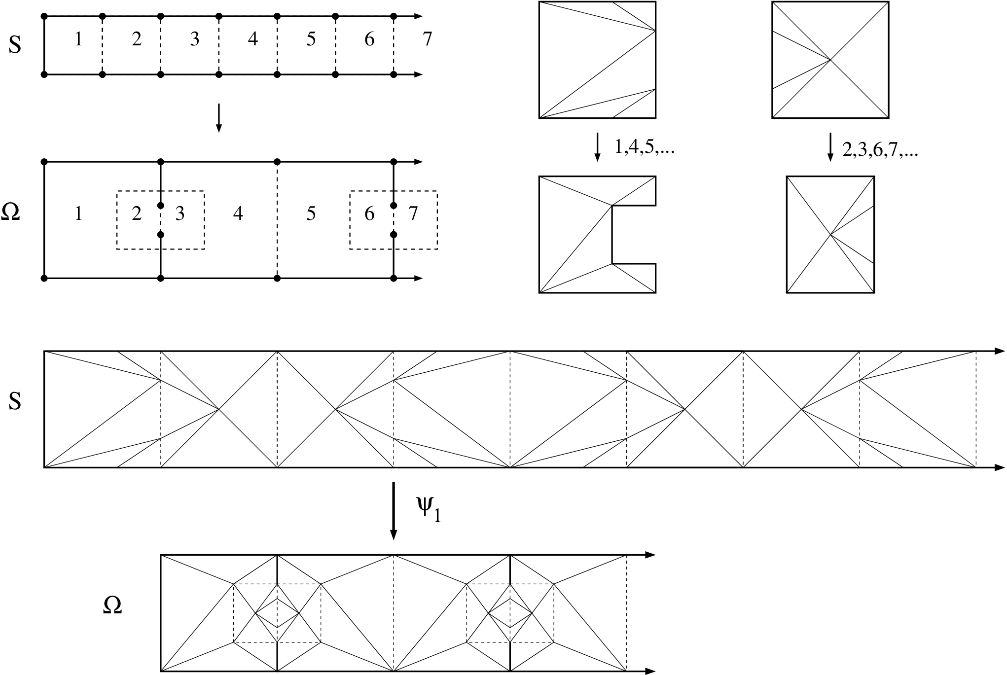
Now for the example. Consider Figure 4. It shows the half-strip $S$ and a subdomain $\Omega\subset S$ formed by removing certain vertical slits from $S$. Both $S$ and $\Omega$ are partitioned into pieces that are numbered $1,2,3,\dots$ moving left to right. The pieces of $S$ are all squares. The pieces of $\Omega$ have two shapes: rectangles and pieces that look like a letter “C” or its reflection. Figure 4 shows a triangulation for each piece and we can easily check that corresponding pieces for $S$ and $\Omega$ have compatible triangulations. Using these building blocks we can find compatible triangulations of all of $S$ and $\Omega$ and hence a piecewise linear map from $S$ to $\Omega$. Since we are repeatedly using just two building blocks, the map is quasiconformal, with constant determined by the most distorted triangle from a finite set of possibilities. Note that the particular choice of triangulation is not important, and we have made no attempt to optimize the number of triangles used or the resulting QC constant.

The map $\psi_{1}$ is linear on a partition ${\cal J}$ of $\partial S$ consisting of equal length segments. We define an exponential partition by dividing the segments on $\partial\Omega$ into sub-segments; about $2^{n}$ for segments that are between distance $n$ and $n+1$ from the left side of $\Omega$. Pulling back these edges on $\partial\Omega$ via $\psi_{1}$ gives an exponential partition of $\partial S$ and then we apply the construction of the Section 3 to build $\psi_{0}$. If $\psi=\psi_{1}\circ\psi_{0}:{\mathbb{H}}_{r}\to\Omega$ then

is defined on $\Omega^{\prime}=\cosh(\Omega)$ and extends to a quasiregular function on the plane. Thus there is a $\phi$ so that $f=g\circ\phi$ is entire with two critical values.

Also note that $f$ has positive, finite order. It has order $\geq 1/2$ simply because all functions in class $\cal B$ do. To show $f$ has finite order it suffices to show $g$ does; the quasiconformal correction can only change the order by a multiple depending on the quasiconformal constant of the correction map $\phi$ (i.e., $\phi$ is Hölder). The main property of $\Omega$ that we need is that it contains a half-strip $\{x+iy:x>0,|y|<w\}$ for some fixed $w>0$.

Suppose $x\geq 2\pi$ and let $D=D(x,r)$ be the maximal disk centered at $x$ contained in $\Omega$. Since $\Omega$ is contained in the strip $S$, we have $r\leq\pi$ and $\partial D$ hits $\partial\Omega$ at symmetric points $t\pm iy$ with $|x-t|\leq\pi$ and $y\geq w$. Let $S_{x}$ be the hyperbolic geodesic in $D$ connecting these two points. This arc cuts $D$ into two subdomains that are quasicircles with uniformly bounded constant, and hence a result of Fernández, Heinonen and Martio [8] implies the image of each of these domains is a quasicircle with uniformly bounded constant in ${\mathbb{H}}_{r}$. This easily implies that $\gamma_{x}=\psi^{-1}(S_{x})$ is a curve in ${\mathbb{H}}_{r}$ that is symmetric with respect to the real line and satisfies $R_{x}\simeq r_{x}\simeq\psi^{-1}(x)$ where

(In other words, $\gamma$ is contained in an annulus around the origin of fixed modulus, independent of $x$.) See Figure 5.

If $I$ is the left side of $\Omega$ then the extremal distance from $\psi^{-1}(I)$ to $\gamma_{x}$ in ${\mathbb{H}}_{r}$ is comparable to the extremal distance from $I$ to $S_{x}$ in $\Omega$ (since modulus is quasi-preserved by $\psi$). The first is easily seen to be comparable to $\log R_{x}$ and the second is comparable to $x$, since $\Omega$ is contained in the half-strip $S$ and contains another half-strip of positive width. Finally,

and our previous remarks show the rightmost term is bounded as $x\to\infty$.

More generally, this argument shows that $g$ (and hence $f$) will have finite order whenever the domain $\Omega$ contains an infinite half-strip of positive width.

The domain $\Omega$ used in the proof of Theorem 1.1 is illustrated in Figure 6. It consists of the half-strip $S$ with finite trees removed along the integer points of the top and bottom edge. The domain is symmetric with respect to the real axis and in most of our pictures we will only show the lower half to simplify the illustrations. Note that there is a half-strip contained in $\Omega$; this implies that the function we eventually obtain will have positive, finite order by our previous comments.

Every removed tree contains a vertical unit line segment attached to $\partial S$. For $n=1$ this segment is the entire tree. For $n=2$ we add two segments: another vertical line segment of length $1$ and a diagonal segment of slope $1$ and length $\sqrt{2}$ (so the degree one vertices of the resulting tree are both distance $2$ from $\partial S$). In general, the tree $T_{n}$ attached at the $n$th point is the vertical segment plus a binary tree of depth $n-1$ as shown in Figure 6.

The edges of $T_{n}$ are naturally divided into levels from $0$ (attached to $\partial S$) to $n-1$ (adjacent to the leaves of the tree). We form a new tree $T_{n}^{\prime}$ by subdividing edges in the $k$th level of $T_{n}$ into $4^{k}$ equal sub-edges. See Figure 7. Note that edges in the $k$-th level have length $\simeq 2^{-k}\cdot 4^{-k}=8^{-k}$. We define the vertices of $\partial\Omega$ to correspond to the vertices of $T_{n}^{\prime}$. It is these new, shorter edges that will eventually be mapped to segments of length $\pi/2$ on $\partial{\mathbb{H}}_{r}$. We also subdivide the edges of $\partial\Omega$ on $\partial S$ by adding vertices where the real parts equal $n+\frac{1}{2}$, $n=1,2,3\dots$ along the top and bottom edges of $T$ and adding the points $\pm i\pi/2$ to the left side of $S$.

This subdivision of $T_{n}$ to obtain $T_{n}^{\prime}$ is important for two reasons. First, when we define the map $\psi_{1}:S\to\Omega$, these new edges will pull back to an exponential partition of $\partial S$, and this allows us to define $\psi_{0}$ as before. Second, since every edge of $T_{n}$ of level $k$ is divided into $4^{k}$ sub-edges, we can label the vertices of $T_{n}^{\prime}$ so that the vertices of $T_{n}$ all get label $1$, except for the root of $T_{n}$ (the point where it is attached to $\partial S$) that gets label $0$. Moreover, the roots of the trees are the only vertices labeled zero that are not degree 2 vertices. Hence these are the only preimages of $0$ that are critical points. This fact will be important when we construct a quasiconformal deformation that changes the order of our function.

Next we have to describe the map $\psi_{1}:S\to\Omega$. Consider the dashed curve $\gamma$ in Figure 8. It is horizontal along the top of each tree and has slope $1/2$ between trees (because the horizontal distance between $T_{n}$ and $T_{n+1}$ is $2^{-n+1}$ and $T_{n+1}$ is $2^{-n}$ “taller” than $T_{n}$. The curve $\gamma$ and its reflection across the real line bound a region $\Omega_{1}\subset\Omega$ (half of $\Omega_{1}$ is the shaded region in Figure 8). It is easy to map $S$ to $\Omega_{1}$ by a piecewise linear quasiconformal map that sends $S\cap L$ affinely to $\Omega_{1}\cap L$ for every vertical line $L$.

The leaves of $\partial\Omega$ lie on $\partial\Omega_{1}$ and divide it into segments. We associate each such segment $I$ to a region $Q_{I}\subset\Omega_{1}$. See Figure 9. If $I$ is horizontal, then $Q_{I}$ is the square in $\Omega_{1}$ with $I$ as one side. If $I$ has slope $1/2$ then $Q_{I}$ is the right triangle in $\Omega_{1}$ with hypotenuse $I$ and vertical and horizontal legs. We also associate to $I$ the component $U_{I}$ of $\Omega\setminus\Omega_{1}$ that has $I$ on its boundary.

We let $W_{I}=Q_{I}\cup U_{I}\cup I$ be the union of the regions above and below $I$. We will define a map $\Omega_{1}\to\Omega$ by mapping each region $Q_{I}$ to $W_{I}$. Our map will be the identity on $\partial Q_{I}\cap\Omega_{1}$, and hence extends continuously to all of $\Omega_{1}$ by setting it to the identity outside all the $Q_{I}$’s. This map is called a “filling” map for $W_{I}$.

There are five cases to consider: two special cases that occur once each, and three cases that occur infinitely often. The two special cases are the first two segments on $\gamma$; the ones that project vertically to $[0,1]$ and $[1,2]$. Figures 11 and 12 show how to define these maps using triangulations.

The remaining three cases are illustrated in Figures 13-17. We refer to these cases as triangles ($U_{I}$ is a triangle), partial tubes ($U_{I}$ is not a triangle and does not touch $\partial S$) and full tubes ($U_{I}$ touches $\partial S$). See cases 3, 4 and 5 in Figure 10.

The filling map for full tubes is illustrated in Figures 14 and 15. In Figure 14, the left side shows the region $Q_{I}$ divided into a number of subregions; a pentagon on top, a series of non-convex hexagons and a final triangle. The exact sizes of these regions is important and will be discussed in the next paragraph; for the moment, just assume that each of the middle regions (the non-convex hexagons) is similar to all the others. The regions are labeled with numbers indicating their levels; these are the same levels we used to subdivide the edges of the tree $T_{n}$ to obtain the tree $T_{n}^{\prime}$.

The right side of Figure 14 shows the region $W_{I}$ divided into subregions corresponding to the subregions of $Q_{I}$: a rectangle on top (this contains $Q_{I}$), a series of trapezoids, and a square on the bottom. The regions on left and right are numbered and each subregion on the left is mapped to the corresponding subregion on the right by a piecewise affine map. The triangulations that define this map are illustrated in Figure 15. Because we are only using three basic shapes (even though the middle shape may be used many times), each with a finite triangulation, the maps we build are clearly uniformly quasiconformal.

There is another property we need to check. The partition of the tree into edges is supposed to pull back to an exponential partition of the strip. This means that the vertices along the boundary of a full tube should pull back to a points on $I$ that are approximately evenly spaced and grow exponentially with the distance of $I$ from the left side of $\Omega$. Consider Figure 14. The full tube is pictured on the right and divided into levels (starting with the square on the bottom, which is level 0). The sides of level $k$ are divided into $4^{k}$ equal length edges of the tree (see Figure7). These points pull back to $4^{k}$ equally spaced points on a subsegment of $I$ (on the left of Figure 14, the segment is where the boundary of a subregion hits $I$). In order for the collection of all preimage points to be equally spaced on $I$, we need each segment corresponding to a level $k$ region to be $4$ times longer than the segments corresponding to a level $k-1$ region, but this is easy to accomplish. This implies that when the edges of $\partial\Omega$ are pulled back, every preimage in $[n,n+1]$ has length $\simeq 4^{-n}$ and hence they form an exponential partition.

The corresponding pictures for partial tubes are a little simpler. Figure 16 shows how we cut $Q_{i}$ and $W_{I}$ into corresponding pieces and Figure 17 shows how each piece is mapped via a triangulation. The rest of the argument is the same as for the full tubes (checking the map is uniformly quasiconformal and defines an exponential partition of the strip).

This completes our construction of the quasiregular map $g=\cosh\circ\,\psi^{-1}\circ\cosh^{-1}$ and hence of an entire function $f=g\circ\phi$ with three singular values. The next section will prove $f$ is a counterexample to the order conjecture.

Suppose $f$ is the entire function constructed in the previous section. We claim we can choose quasiconformal maps $\tau,\sigma$ and an entire function $F$ so that

where $\tau$ is the identity off a compact set and $\sigma$ satisfies

for all sufficiently large $z$.

First we check that (6.1) gives the desired counterexample. Taking $z=\sigma(w)$,

since $f=\tau\circ f$ when $|f|$ is large enough. Thus the order of $F$ is at least twice the order of $f$. Since the order of $f$ is positive and finite, the two orders are different.

Now we prove the claims. First we define $\tau$. Let $W=D(1,2)\setminus[0,1]$. $W$ is a topological annulus and is conformally equivalent to the round annulus $A_{t}=\mathbb{D}\setminus t\mathbb{D}$ for some $t$. For $K>1$, the map

is a $K$-quasiconformal from $A_{t}$ to $A_{t^{K}}$ that is the identity on the outer boundary of $A_{t}$ and decreases the extremal length of the path family that separates the two boundary components of $A$ by a factor of $K$. Let $W_{K}$ be the domain of the form $D(1,2)\setminus[s,1]$ that is conformally equivalent to $A^{t^{K}}$. Thus $r_{K}$ transfers to a $K$-quasiconformal map $\tau:W\to W_{K}$ that is the identity on the outer boundary of $W$ decreases the extremal length of the path family that separates the two boundary components of $A$ by a factor of $K$. It is easy to check that $\tau$ extends continuously across the slit boundary of $W$ and can be extended by the identity outside $\overline{W}$ to give a $K$-quasiconformal map of the whole plane. This is the map $\tau$ we use in our quasiconformal equivalence. By the measurable Riemann mapping theorem, there is a $K$-quasiconformal map $\sigma$ of the plane so that $F=\tau\circ f\circ\sigma$ is entire. We can assume $\sigma$ fixes $-1,1,\infty$.

All that remains is to show that (6.1) holds. Let $V=D(1,2)\setminus[-1,1]$ and consider inverse images of $V$ under $f$. By construction, every such preimage contains two preimages of $0$ on its boundary and either
    (I) both preimages are critical points,
    (II) exactly one preimage is a critical point, or
    (III) neither preimage is a critical point.
Case I occurs when the preimages of zero are the roots of two adjacent trees. Case II only occurs twice and corresponds to the corners of $S$ in $\cosh$ coordinates. Case III occurs for preimages that do not touch $\partial S$ in $\cosh$ coordinates. A cartoon of the different types of preimages is shown (in $\cosh$ coordinates) in Figure 18.

Let $\gamma_{0}=[-i\pi/2,i\pi/2]$ and for $n=1,2,\dots$ let $\gamma_{n}$ be the vertical crosscut of $S$ that contains the point where the $n$th tree is attached. Let $\Gamma_{n}$ be the path family connecting $\gamma_{0}$ to $\gamma_{n}$ inside the closure of the type I and type II components. This family has extremal length $\leq Mn$ for some fixed $M$.

Applying $\cosh$, $\gamma_{n}$, $n\geq 1$, maps to an ellipse $E_{n}$ of bounded eccentricity and diameter $\simeq e^{n}$. Also, $\cosh(\Gamma_{n})$ is a family of paths connecting $[0,1]$ to $E_{n}$. Let $V_{n}$ be the region bounded by the ellipse $E_{n}$, minus $[-1,1]$ and let $\Sigma_{n}$ be the path family in $V_{n}$ connecting $[-1,1]$ to $E_{n}$. Then $\Sigma_{n}$ contains $\cosh(\Gamma_{n})$, and $V_{n}\setminus(-\infty,-1]$ is conformally equivalent to a $2\pi\times n$ rectangle, so if $\lambda$ denotes extremal length we get

When we apply the quasiconformal map $\sigma$, the extremal length of $\Gamma_{n}$ is reduced by a factor of $K$; this is exactly why we choose $\tau$ as we did. Hence

if $K$ is large enough. The eccentricity of the ellipse $E_{n}$ tends to $1$ as $n\nearrow\infty$ so $\sigma(E_{n})$ is a $2K$-quasicircle when $n$ is large enough. Let

Since $\{1\leq|z|\leq r\}\subset\sigma(V_{n})$, we have $\frac{1}{2\pi}\log r\leq\lambda(\sigma(\Sigma_{n}))\leq Mn/K$, and hence

if $K\geq 4\pi M$. Quasiconformal maps are quasisymmetric, so we have $R\leq C_{K}\cdot r$ for some constant depending only on $K$ and hence $R\leq C_{K}\cdot e^{n/2}.$ If $z\in V_{n}\setminus V_{n-1}$, then

which is (6.1). This proves Theorem 1.1, i.e., the order conjecture fails in $\cal S$.

References

- [1] Lars V. Ahlfors. Lectures on quasiconformal mappings, volume 38 of University Lecture Series. American Mathematical Society, Providence, RI, second edition, 2006. With supplemental chapters by C. J. Earle, I. Kra, M. Shishikura and J. H. Hubbard.
- [2] Walter Bergweiler and Alexandre Eremenko. On the singularities of the inverse to a meromorphic function of finite order. Rev. Mat. Iberoamericana, 11(2):355–373, 1995.
- [3] Christopher J. Bishop. Constructing entire functions by quasiconformal folding. preprint 2011.
- [4] Adam L. Epstein. Finite order entire functions and meromorphic quadratic differentials. preprint 2007.
- [5] Adam L. Epstein and Lasse Rempe. On the invariance of order for finite-type entire functions. preprint 2012.
- [6] A. E. Eremenko and M. Yu. Lyubich. Dynamical properties of some classes of entire functions. Ann. Inst. Fourier (Grenoble), 42(4):989–1020, 1992.
- [7] Alex Eremenko. Geometric theory of meromorphic functions. preprint 2006.
- [8] José L. Fernández, Juha Heinonen, and Olli Martio. Quasilines and conformal mappings. J. Analyse Math., 52:117–132, 1989.
- [9] Peter W. Jones. On removable sets for Sobolev spaces in the plane. In Essays on Fourier analysis in honor of Elias M. Stein (Princeton, NJ, 1991), volume 42 of Princeton Math. Ser., pages 250–267. Princeton Univ. Press, Princeton, NJ, 1995.
- [10] Peter W. Jones and Stanislav K. Smirnov. Removability theorems for Sobolev functions and quasiconformal maps. Ark. Mat., 38(2):263–279, 2000.
- [11] Hans P. Künzi. Konstruktion Riemannscher Flächen mit vorgegebener Ordnung der erzeugenden Funktionen. Math. Ann., 128:471–474, 1955.
- [12] J. K. Langley. On the multiple points of certain meromorphic functions. Proc. Amer. Math. Soc., 123(6):1787–1795, 1995.
- [13] Gwyneth M. Stallard. Dimensions of Julia sets of hyperbolic meromorphic functions. Bull. London Math. Soc., 33(6):689–694, 2001.