A Novel Approach to Generate Correctly Rounded Math Libraries for New Floating Point RepresentationsJournal: PACMPLVolume: 1Rutgers Computer Science Technical Report7537

The FP representation $\mathbb{F}_{n,|E|}$, which is specified in the IEEE-754 standard (Cowlishaw 2008), is parameterized by the total number of bits $n$ and the number of bits for the exponent $|E|$. There are three components in a FP bit-string: a sign bit $s$, $|E|$-bits to represent the exponent, and $|F|$-bits to represent the mantissa $F$ where $|F|=n-1-|E|$. Figure 2(a) shows the FP format. If $s=0$, then the value is positive. If $s=1$, then the value is negative. The value represented by the FP bit-string is a normal value if the bit-string $E$, when interpreted as an unsigned integer, satisfies $0<E<2^{|E|}-1$. The normal value represented with this bit-string is $(1+\frac{F}{2^{|F|}})\times 2^{E-bias}$, where bias is $2^{|E|-1}-1$. If $E=0$, then the FP value is a denormal value. The value of the denormal value is $(\frac{F}{2^{|F|}})\times 2^{1-bias}$. When $E=2^{|E|}-1$, the FP bit-strings represent special values. If $F=0$, then the bit-string represents $\pm\infty$ depending on the value of $s$ and in all other cases, it represents not-a-number (NaN).

IEEE-754 specifies a number of default FP types: 16-bit ($\mathbb{F}_{16,5}$ or half), 32-bit ($\mathbb{F}_{32,8}$ or float), and 64-bit ($\mathbb{F}_{64,11}$ or double). Beyond the types specified in the IEEE-754 standard, recent extensions have increased the dynamic range and/or precision. Bfloat16 (Tagliavini et al. 2018), $\mathbb{F}_{16,8}$, provides increased dynamic range compared to FP’s half type. Figure 2(b) illustrates the Bfloat16 format. Recently proposed TensorFloat32 (NVIDIA 2020), $\mathbb{F}_{19,8}$, increased both the dynamic range and precision compared to the half type.

Posit (Gustafson 2017; Gustafson and Yonemoto 2017) is a new representation that provides tapered precision with a fixed number of bits. A posit representation, $\mathbb{P}_{n,es}$, is defined by the total number of bits $n$ and the maximum number of bits for the exponents $es$. A posit bit-string consists of five components (see Figure 2(d)): a sign bit $s$, a number of regime bits $R$, a regime guard bit $\overline{R}$, up to $es$-bits of the exponent $E$, and fraction bits $F$. When the regime bits are not used, they can be re-purposed to represent the fraction, which provides tapered precision.

Value of a posit bit-string. The first bit is a sign bit. If $s=0$, then the value is positive. If $s=1$, then the value is negative and the bit-string is decoded after taking the two’s complement of the remaining bit-string after the sign bit. Three components $R$, $\overline{R}$, and $E$ together are used to represent the exponent of the final value. After the sign bit, the next $1\leq|R|\leq n-1$ bits represent the regime $R$. Regime bits consist of consecutive $1$’s (or $0$’s) and are only terminated if $|R|=n-1$ or by an opposite bit $0$ (or $1$), which is known as the regime guard bit ($\overline{R}$). The regime bits represent the super exponent. Regime bits contribute $useed^{r}$ to the value of the number where $useed=2^{2^{es}}$ and $r=|R|-1$ if $R$ consists of 1’s and $r=-|R|$ if $R$ consists of 0’s.

If $2+|R|<n$, then the next $min\{es,n-2-|R|\}$ bits represent the exponent bits. If $|E|<es$, then $E$ is padded with $0$’s to the right until $|E|=es$. These $|es|$-bits contribute $2^{E}$ to the value of the number. Together, the regime and the exponent bits of the posit bit-string contribute $useed^{r}\times 2^{E}$ to the value of the number. If there are any remaining bits after the $es$-exponent bits, they represent the fraction bits $F$. The fraction bits are interpreted like a normal FP value, except the length of $F$ can vary depending on the number of regime bits. They contribute $1+\frac{F}{2^{|F|}}$. Finally, the value $v$ represented by a posit bit-string is,

There are two special cases. A bit-string of all $0$’s represents $0$. A bit-string of $1$ followed by all $0s$’s represents Not-a-Real (NaR).

Example. Consider the bit-string 0000011011000000 in the $\mathbb{P}_{16,1}$ configuration. Here, $useed=2^{2^{1}}=2^{2}$. Also $s=$ 0, $R=$ 0000, $\overline{R}=$ 1, $E=$ 1, and $F=$ 011000000. Hence, $r=-|R|=-4$. The final exponent resulting from the regime and the exponent bits is $(2^{2})^{-4}\times 2^{1}=2^{-7}$. The fraction value is $1.375$. The value represented by this posit bit-string is $1.375\times 2^{-7}$.

When a real number $x$ cannot be represented in a target representation $\mathbb{T}$, it has to be rounded to a value $v\in\mathbb{T}$. The FP standard defines a number of rounding modes but the default rounding mode is the round-to-nearest-tie-goes-to-even (RNE) mode. The posit standard also specifies RNE rounding mode with a minor difference that any non-zero value does not underflow to 0 or overflow to NaR. We describe our approach with RNE mode but it is applicable to other rounding modes.

In the RNE mode, the rounding function $v=RN_{\mathbb{T}}(x)$, rounds $x\in\mathbb{R}$ (Reals) to $v\in\mathbb{T}$, such that $x$ is rounded to the nearest representable value in $\mathbb{T}$, i.e. $\forall_{v^{\prime}\in\mathbb{T}}|x-v|\leq|x-v^{\prime}|$. In the case of a tie, where $\exists{v_{1},v_{2}\in\mathbb{T},v_{1}\neq v_{2}}$ such that $|x-v_{1}|=|x-v_{2}|$ and $\forall_{v^{\prime}\in\mathbb{T}}|x-v_{1}|\leq|x-v^{\prime}|$, then $x$ is rounded to $v_{1}$ if the bit-string encoding the value $v_{1}$ is an even number when interpreted as an integer and to $v_{2}$ otherwise. Figure 3 illustrates the RNE mode with a 5-bit FP representation from Figure 2(c).

The result of primitive operations in FP or any other representation experiences rounding error when it cannot be exactly represented. Modern hardware and libraries produce correctly rounded results for primitive operations. However, this rounding error can get amplified with a series of primitive operations because the intermediate result of each primitive operation must be rounded. As math libraries are also implemented with finite precision, numerical errors in the implementation should also be carefully addressed.

The state-of-the-art methods to approximate an elementary function $f(x)$ for a target representation ($\mathbb{T}$) involves two steps. First, approximation theory (e.g., minimax methods) is used to develop a function $A_{\mathbb{R}}(x)$ that closely approximates $f(x)$ using real numbers. Second, $A_{\mathbb{R}}(x)$ is implemented in a finite precision representation that has higher precision than $\mathbb{T}$.

Generating $A_{\mathbb{R}}(x)$. Mathematically deriving $A_{\mathbb{R}}(x)$ can be further split into three steps. First, identify inputs that exhibit special behavior (e.g., $\pm\infty$). Second, reduce the input domain to a smaller interval, $[a^{\prime},b^{\prime}]$, with range reduction techniques and perform any other function transformations. Third, generate a polynomial $P(x)$ that approximates $f(x)$ in the domain $[a^{\prime},b^{\prime}]$.

There are two types of special cases. The first type includes inputs that produce undefined values or $\pm\infty$ when mathematically evaluating $f(x)$. For example, in the case of $f(x)=10^{x}$, $f(x)=\infty$ if $x=\infty$. The second type consists of interesting inputs for evaluating $RN_{\mathbb{T}}(f(x))$. These cases include a range of inputs that produce interesting outputs such as $RN_{\mathbb{T}}(f(x))\in\{\pm\infty,0\}$. For example, while approximating $f(x)=10^{x}$ for Bfloat16 ($\mathbb{B}$), all values $x\in(-\infty,-40.5]$ produce $RN_{\mathbb{B}}(10^{x})=0$, inputs $x\in[-8.46\dots\times 10^{-4},1.68\dots\times 10^{-3}]$ produce $RN_{\mathbb{B}}(10^{x})=1$, and $x\in[38.75,\infty)$ produces $RN_{\mathbb{B}}(10^{x})=\infty$. These properties are specific to each $f(x)$ and $\mathbb{T}$.

Range reduction. It is mathematically simpler to approximate $f(x)$ for a small domain of inputs. Hence, most math libraries use range reduction to reduce the entire input domain into a smaller domain before generating the polynomial. Given an input $x\in[a,b]$ where $[a,b]\subseteq\mathbb{T}$, the goal of range reduction is to reduce the input $x$ to $x^{\prime}\in[a^{\prime},b^{\prime}]$, where $[a^{\prime},b^{\prime}]\subset[a,b]$. We represent this process of range reduction with $x^{\prime}=RR(x)$. Then, the polynomial $P$ approximates the output $y^{\prime}$ for the range reduced input (i.e., $y^{\prime}=P(x^{\prime})$). The output ($y^{\prime}$) of the range reduced input ($x^{\prime}$) has to be compensated to produce the output for the original input ($x$). The output compensation function, $OC(y^{\prime},x)$, produces the final result by compensating the range reduced output $y^{\prime}$ based on the range reduction performed for input $x$.

For example, consider the function $f(x)=log_{2}(x)$ where the input domain is defined over $(0,\infty)$. One way to range reduce the original input is to use the mathematical property $log_{2}(a\times 2^{b})=log_{2}(a)+b$. We decompose the input $x$ as $x=x\textquoteright\times 2^{e}$ where $x\textquoteright\in[1,2)$ and $e$ is an integer. Approximating $log_{2}(x)$ is equivalent to approximating $log_{2}(x\textquoteright\times 2^{e})=log_{2}(x\textquoteright)+e$. Thus, we can range reduce the original input $x\in(0,\infty)$ into $x\textquoteright\in[1,2)$. Then, we approximate $log_{2}(x\textquoteright)$ using $P(x\textquoteright)$, which needs to only approximate $log_{2}(x)$ for the input domain $[1,2)$. To produce the output of $log_{2}(x)$, we compensate the output of the reduced input by computing $P(x^{\prime})+e$, where $e$ is dependent on the range reduction of $x$.

Polynomial approximation $P(x)$. A common method to approximate an elementary function $f(x)$ is with a polynomial function, $P(x)$, which can be implemented with addition, subtraction, and multiplication operations. Typically, $P(x)$ for math libraries is generated using the minimax approximation technique, which aims to minimize the maximum error, or $L_{\infty}$-norm,

where $\sup$ represents the supremum of a set. The minimax approach is attractive because the resulting $P(x)$ has a bound on the error (i.e., $|P(x)-f(x)|$). The most well-known minimax approximation method is the Remez algorithm (Remes 1934). Both CR-LIBM (Daramy et al. 2003) and Metalibm (Kupriianova and Lauter 2014) use a modified Remez algorithm to produce polynomial approximations (Brisebarre and Chevillard 2007).

Implementation of $A_{\mathbb{R}}(x)$ with finite precision. Finally, mathematical approximation $A_{\mathbb{R}}(x)$ is implemented in finite precision to approximate $f(x)$. This implementation typically uses a higher precision than the intended target representation. We use $A_{\mathbb{H}}(x)$ to represent that $A_{\mathbb{R}}(x)$ is implemented in a representation with higher precision ($\mathbb{H}$) where $\mathbb{T}\subset\mathbb{H}$. Finally, the result of the implementation $A_{\mathbb{H}}(x)$ is rounded to the target representation $\mathbb{T}$.

An approximation of an elementary function $f(x)$ is defined to be a correctly rounded approximation if for all inputs $x_{i}\in\mathbb{T}$, it produces $RN_{\mathbb{T}}(f(x_{i}))$. There are two major challenges in creating a correctly rounded approximation. First, $A_{\mathbb{H}}(x)$ incurs error because $P(x)$ is an approximation of $f(x)$. Second, the evaluation of $A_{\mathbb{H}}(x)$ has numerical error because it is implemented in a representation with finite precision (i.e., $\mathbb{H}$). Hence, the rounding of $RN_{\mathbb{T}}(A_{\mathbb{H}}(x))$ can result in a value different from $RN_{\mathbb{T}}(f(x))$, even if $A_{\mathbb{H}}(x)$ is arbitrarily close to $f(x)$ for some $x\in\mathbb{T}$.

As $A_{\mathbb{R}}(x)$ uses a polynomial approximation of $f(x)$, there is an inherent error of $|f(x)-A_{\mathbb{R}}(x)|>0$. Further, the evaluation of $A_{\mathbb{H}}(x)$ experiences an error of $|A_{\mathbb{H}}(x)-A_{\mathbb{R}}(x)|>0$. It is not possible to reduce both errors to 0. The error in approximating the polynomial can be reduced by using a polynomial of a higher degree or a piece-wise polynomial. The numerical error in the evaluation of $A_{\mathbb{H}}(x)$ can be reduced by increasing the precision of $\mathbb{H}$. Typically, library developers make trade-offs between error and the performance of the implementation.

Unfortunately, there is no known general method to analyze and predict the bound on the error for $A_{\mathbb{H}}(x)$ that guarantees $RN_{\mathbb{T}}(A_{\mathbb{H}}(x))=RN_{\mathbb{T}}(f(x))$ for all $x$ because the error may need to be arbitrarily small. This problem is widely known as table-maker’s dilemma (Kahan 2004). It states that there is no general method to predict the amount of precision in $\mathbb{H}$ such that the result is correctly rounded for $\mathbb{T}$.

An alternative to developing math libraries for new representations is to use existing libraries. We can convert the input $x\in{\mathbb{T}}$ to $x^{\prime}=RN_{\mathbb{T^{\prime}}}(x)$, , where $\mathbb{T}$ is the representation of interest and $\mathbb{T^{\prime}}$ is the representation that has a math library available (e.g., double). Subsequently, we can use a math library for $\mathbb{T^{\prime}}$ and round the result back to $\mathbb{T}$. This strategy is appealing if a correctly rounded math library for $\mathbb{T^{\prime}}$ exists and $\mathbb{T^{\prime}}$ has significantly more precision bits than $\mathbb{T}$.

However, using a correctly rounded math library designed for $\mathbb{T^{\prime}}$ to approximate $f(x)$ for $\mathbb{T}$ can produce incorrect results for values in $\mathbb{T}$. We illustrate this behavior by generating an approximation for the function $f(x)=10^{x}$ in the Bfloat16 ($\mathbb{B}$) representation (Figure 4). Let’s consider the input $x=-0.0181884765625\in\mathbb{B}$. The real value of $f(x)\approx 0.95898435797\dots$ (black circle in Figure 4). This oracle result cannot be exactly represented in Bfloat16 and must be rounded. There are two Bfloat16 values adjacent to $f(x)$, $b_{1}=0.95703125$ and $b_{2}=0.9609375$. Since $b_{1}$ is closer to $f(x)$, the correctly rounded result is $RN_{\mathbb{B}}(10^{x})=b_{1}$, which is represented by a black star in Figure 4.

If we use the correctly rounded float math library to approximate $10^{x}$, we get the value, $y^{\prime}=0.958984375$, represented by red diamond in Figure  4. From the perspective of a 32-bit float, $y^{\prime}$ is a correctly rounded result, i.e. $y^{\prime}=RN_{\mathbb{F}_{32,8}}(10^{x})=0.958984375$. Because $y^{\prime}\notin\mathbb{B}$, we round $y^{\prime}$ to Bfloat16 based on the rounding rule, $RN_{\mathbb{B}}(y^{\prime})=b_{2}$. Therefore, the float math library rounds the result to $b_{2}$ but the correctly rounded result is $RN_{\mathbb{B}}(10^{x})=b_{1}$.

Summary. Approximating an elementary function for representation $\mathbb{T}$ using a math library designed for a higher precision representation $\mathbb{T^{\prime}}$ does not guarantee a correctly rounded result. Further, the math library for $\mathbb{T^{\prime}}$ probably requires higher accuracy than the one for $\mathbb{T}$. Hence, it uses a higher degree polynomial, which causes it to be slower than the math library tailored for $\mathbb{T}$.

Given an elementary function $f(x)$ and a target representation $\mathbb{T}$, our goal is to synthesize a polynomial that when used with range reduction ($RR$) and output compensation ($OC$) function produces the correctly rounded result for all inputs in $\mathbb{T}$. The evaluation of the polynomial, range reduction, and output compensation are implemented in representation $\mathbb{H}$, which has higher precision than $\mathbb{T}$.

Our methodology for generating correctly rounded elementary functions is shown in Figure 1. Our methodology consists of four steps. First, we use an oracle (i.e., MPFR (Fousse et al. 2007) with a large number of precision bits) to compute the correctly rounded result of the function $f(x)$ for each input $x\in\mathbb{T}$. In this step, a small sample of the entire input space can be used rather than using all inputs for a type with a large input domain.

Second, we identify an interval $[l,h]$ around the correctly rounded result such that any value in $[l,h]$ rounds to the correctly rounded result in $\mathbb{T}$. We call this interval the rounding interval. Since the eventual polynomial evaluation happens in $\mathbb{H}$, the rounding intervals are also in the $\mathbb{H}$ representation. The internal computations of the math library evaluated in $\mathbb{H}$ should produce a value in the rounding interval for each input $x$.

Third, we employ range reduction to transform input $x$ to $x^{\prime}$. The generated polynomial will approximate the result for $x^{\prime}$. Subsequently, we have to use an appropriate output compensation code to produce the final correctly rounded output for $x$. Both range reduction and output compensation happen in the $\mathbb{H}$ representation and can experience numerical errors. These numerical errors should not affect the generation of correctly rounded results. Hence, we infer intervals for the reduced domain so that the polynomial evaluation over the reduced input domain produces the correct results for the entire domain. Given $x$ and its rounding interval $[l,h]$, we can compute the reduced input $x^{\prime}$ with range reduction. The next task before polynomial generation is identifying the reduced rounding interval for $P(x^{\prime})$ such that when used with output compensation it produces the correctly rounded result. We use the inverse of the output compensation function to identify the reduced interval $[l^{\prime},h^{\prime}]$. Any value in $[l^{\prime},h^{\prime}]$ when used with the implementation of output compensation in $\mathbb{H}$ produces the correctly rounded results for the entire domain.

Fourth, we synthesize a polynomial of a degree $d$ using an arbitrary precision linear programming (LP) solver that satisfies the constraints (i.e., $l^{\prime}\leq P(x^{\prime})\leq h^{\prime}$) when given a set of inputs $x^{\prime}$. Since the LP solver produces coefficients for the polynomial in arbitrary precision, it is possible that some of the constraints will not be satisfied when evaluated in $\mathbb{H}$. In such cases, we refine the reduced intervals for those inputs whose constraints are violated and repeat the above step. If the LP solver is not able to produce a solution, then the developer of the library has to either increase the degree of the polynomial or reduce the input domain.

If the inputs were sampled in the first step, we check whether the generated polynomial produces the correctly rounded result for all inputs. If it does not, then the input is added to the sample and the entire process is repeated. At the end of this process, the polynomial along with range reduction and output compensation when evaluated in $\mathbb{H}$ produces the correctly rounded outputs for all inputs in $\mathbb{T}$.

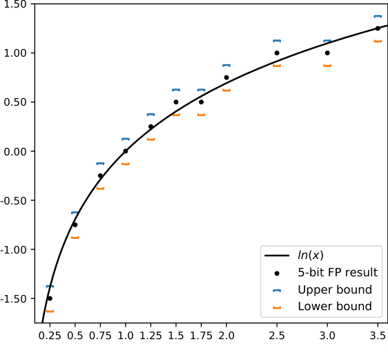
We provide an end-to-end example of our approach by creating a correctly rounded result of $ln(x)$ for the FP5 representation shown in Figure 2(c) with the RNE rounding mode. The $ln(x)$ function is defined over the input domain $(0,\infty)$. There are 11 values ranging from $0.25$ to $3.5$ in FP5 within $(0,\infty)$. We show the generation of the polynomial with FP5 for pedagogical reasons. With FP5, it is beneficial to create a pre-computed table of correctly rounded results for the 11 values.

Our strategy is to approximate $ln(x)$ by using $log_{2}(x)$. Hence, we perform range reduction and output compensation using the properties of logarithm: $ln(x)=\frac{log_{2}(x)}{log_{2}(e)}$ and $log_{2}(x\times y^{z})=log_{2}(x)+zlog_{2}(y)$. We decompose the input $x$ as $x=x^{\prime}\times 2^{n}$ where $x^{\prime}$ is the fractional value represented by the mantissa, i.e. $x^{\prime}\in[1,2)$, and $n$ is the exponent of the value. We use $ln(x)=\frac{log_{2}(x^{\prime})+m}{log_{2}(e)}$ for our range reduction. We construct the range reduction function $RR(x)$ and the output compensation function $OC(y^{\prime},x)$ as follows,

where $fr(x)$ returns the fractional part of $x$ (i.e., $x^{\prime}\in[1,2)$) and $exp(x)$ returns the exponent of $x$ (i.e., $n$). Then, our polynomial approximation $P(x^{\prime})$ should approximate the function $log_{2}(x)$ for the reduced input domain $x^{\prime}\in[1,2)$. The various steps of our approach are illustrated in Figure 5.

Step 1: Identifying the correctly rounded result. There are a total of 11 FP5 values in the input domain of $ln(x)$, $(0,\infty)$. These values are shown on the x-axis in Figure 5(a). Other values are special cases. They are captured by the precondition for this function (i.e., $x=0$ or $x=\infty$). Our goal is to generate the correctly rounded results for these 11 FP5 values. For each of these 11 inputs $x$, we use an oracle (i.e., MPFR math library) to compute $y$, which is the correctly rounded value of $ln(x)$. Figure 5(a) shows the correctly rounded result for each input as a black dot.

Step 2: Identifying the rounding interval $[l,h]$. The range reduction, output compensation, and polynomial evaluation are performed with the double type. The double result of the evaluation is rounded to FP5 to produce the final result. The next step is to find a rounding interval $[l,h]$ in the double type for each output. Figure 5(a) shows the rounding interval for each FP5 output using the blue (upper bound) and orange (lower bound) bracket.

Let us suppose that we want to compute the rounding interval for $y=1.0$, which is the correctly rounded result of $ln(2.5)$. To identify the lower bound $l$ of the rounding interval for $y=1.0$, we first identify the preceding FP5 value, which is $0.75$. Then we find a value $v$ between $0.75$ and $1.0$ such that values greater than or equal to $v$ rounds to $1.0$. In our case, $v=0.875$, which is the lower bound. Similarly, to identify the upper bound $h$, we identify the FP5 value succeeding $1.0$, which is $1.25$. We find a value $v$ such that any value less than or equal to $v$ rounds to $1.0$. In our case, the upper bound is $h=1.125$. Hence, the rounding interval for $y=1.0$ is $[0.875,1.125]$. Figure 6 shows the intervals for a small subset of FP5.

Step 3-a: Computing the reduced input $x^{\prime}$ and the reduced interval $[l^{\prime},h^{\prime}]$. We perform range reduction and generate a polynomial that computes $log_{2}(x)$ for all reduced inputs in $[1,2)$. The next step is to identify the reduced input and the rounding interval for the reduced input such that it accounts for any numerical error in output compensation. Figure 5(b) shows the reduced input (number below the value on the x-axis) and the reduced interval for each input.

To identify the reduced rounding interval, we use the inverse of the output compensation function, which exists if $OC$ is continuous and bijective over real numbers. For example, for the input $x=3.5=1.75\times 2^{1}$, the output compensation function is,

The inverse is

Thus, we use the inverse output compensation function to compute the candidate reduced interval $[l^{\prime},h^{\prime}]$ by computing $l^{\prime}=OC^{-1}(l,x)$ and $h^{\prime}=OC^{-1}(h,x)$. Then, we verify that the output compensation result of $l^{\prime}$ (i.e., $OC(l^{\prime},x)$) and $h^{\prime}$ (i.e., $OC(h^{\prime},x)$), when evaluated in double lies in $[l,h]$. If it does not, then we iteratively refine the reduced interval by restricting $[l^{\prime},h^{\prime}]$ to a smaller interval until both $OC(l^{\prime},x)$ and $OC(h^{\prime},x)$ evaluated in double results lie in $[l,h]$. The vertical bars in Figure 5(b) show the reduced input for each $x$ and its corresponding reduced rounding interval.

Step 3-b: Combining the reduced intervals. Multiple inputs from the original input domain can map to the same reduced input after range reduction. In our example, both $x_{1}=1.25$ and $x_{2}=2.5$ reduce to $x^{\prime}=1.25$. However, the reduced intervals that we compute for $x_{1}$ and $x_{2}$ are $[l_{1}^{\prime},h_{1}^{\prime}]$ and $[l_{2}^{\prime},h_{2}^{\prime}]$, respectively. They are not exactly the same. In Figure 5(b), the reduced intervals corresponding to the original inputs that map to the same reduced input are colored with the same color. The reduced intervals for $x_{1}=1.25$ and $x_{2}=2.5$ are colored in blue.

The reduced interval for $x_{1}$ indicates that $P(1.25)$ must produce a value in $[l_{1}^{\prime},h_{1}^{\prime}]$ such that the final result, after evaluating the output compensation function in double, is the correctly rounded value of $ln(1.25)$. The reduced interval for $x_{2}$ indicates that $P(1.25)$ must produce a value in $[l_{2}^{\prime},h_{2}^{\prime}]$ such that the final result is the correct value of $ln(2.5)$. To produce the correctly rounded result for both inputs $x_{1}$ and $x_{2}$, $P(1.25)$ must produce a value that is in both $[l_{1}^{\prime},h_{1}^{\prime}]$ and $[l_{2}^{\prime},h_{2}^{\prime}]$. Thus, we combine all reduced intervals that correspond to the same reduced input by computing the common interval. Figure 5(b) shows the common interval for a given reduced input using a darker shade. At the end of this step, we are left with one combined interval for each reduced input.

Step 4: Generating the Polynomial for the reduced input. The combined intervals specify the constraints on the output of the polynomial for each reduced input, which when used with output compensation in double results in a correctly rounded result for the entire domain. Figure 5(c) shows the constraints for $P(x^{\prime})$ for each reduced input.

To synthesize a polynomial $P(x^{\prime})$ of a particular degree (the degree is 1 in this example), we encode the problem as a linear programming (LP) problem that solves for the coefficients of $P(x^{\prime})$. We look for a polynomial that satisfies constraints for each reduced input (Figure 5(d)). We use an LP solver to solve for the coefficients and find $P(x^{\prime})$ with the coefficients in Figure 5(e). The generated polynomial $P(x^{\prime})$ satisfies all the linear constraints as shown in Figure 5(f). Finally, we also verify that the generated polynomial when used with range reduction and output compensation produces the correctly rounded results for all inputs in the original domain.

The first step in our approach is to identify the values that $A_{\mathbb{H}}(x)$ must produce so that the rounded value of $A_{\mathbb{H}}(x)$ is equal to the correctly rounded result of $y=f(x)$, i.e. $RN_{\mathbb{T}}(A_{\mathbb{H}}(x))=RN_{\mathbb{T}}(y)$, for each input $x\in X$. Our key insight is that it is not necessary to produce the exact value of $y$ to produce a correctly rounded result. It is sufficient to produce any value in $\mathbb{H}$ that round to the correct result. For a given rounding mode and an input, we are looking for an interval $I=[l,h]$ around the oracle result that produces the correctly rounded result. We call this the rounding interval.

Given an elementary function $f(x)$ and an input $x\in X$, define a interval $I$ that is representable in $\mathbb{H}$ such that $RN_{\mathbb{T}}(v)=RN_{\mathbb{T}}(f(x))$ for all $v\in I$. If $A_{\mathbb{H}}(x)\in I$, then rounding the result of $A_{\mathbb{H}}(x)$ to $\mathbb{T}$ produces the correctly rounded result (i.e., $RN_{\mathbb{T}}(A_{\mathbb{H}}(x))=RN_{\mathbb{T}}(f(x))$). For each input $x$, if $A_{\mathbb{H}}(x)$ can produce a value that lies within its corresponding rounding interval, then it will produce a correctly rounded result. Thus, the pair $(x,I)$ for each input $x$ defines constraints on the output of $A_{\mathbb{H}}(x)$ such that $RN_{\mathbb{T}}(A_{\mathbb{H}}(x))$ is a correctly rounded result.

Figure 8 presents our algorithm to compute constraints $(x,I)$. For each input $x$ in our input domain $X$, we compute the correctly rounded result of $f(x)$ using an oracle and produce $y$. Next, we compute the rounding interval of $y$ where all values in the interval round to $y$. The rounding interval can be computed as follows. First, we identify $t_{l}$, the preceding value of $y$ in $\mathbb{T}$ (line 11 in Figure  8). Then we find the minimum value $l\in\mathbb{H}$ between $t_{l}$ and $y$ where $l$ rounds to $y$ (line 12 in Figure  8). Similarly for the upper bound, we identify $t_{u}$, the succeeding value of $y$ in $\mathbb{T}$ (line 13 in Figure  8), and find the maximum value $h\in\mathbb{H}$ between $y$ and $t_{u}$ where $h$ rounds to $y$ (line 14 in Figure  8). Then, $[l,h]$ is the rounding interval of $y$ and all values in $[l,h]$ round to $y$. Thus, the pair $(x,[l,h])$ specifies a constraint on the output of $A_{\mathbb{H}}(x)$ to produce the correctly rounded result for input $x$. We generate such constraints for each input in the entire domain (or for a sample of inputs) and produce a list of such constraints (lines 7-9 in Figure  8).

After the previous step, we have a list of constraints, $(x,I)$, that need to be satisfied by our approximation $A_{\mathbb{H}}(x)$ to produce correctly rounded outputs. If we do not perform any range reduction, then we can generate a polynomial that satisfies these constraints. However, it is necessary to perform range reduction ($RR$) in practice to reduce the complexity of the polynomial and to improve performance. Range reduction is accompanied by output compensation ($OC$) to produce the final output. Hence, $A_{\mathbb{H}}(x)=OC_{\mathbb{H}}(P_{\mathbb{H}}(RR_{\mathbb{H}}(x)),x)$. Our goal is to synthesize a polynomial $P_{\mathbb{H}}(x^{\prime})$ that operates on the range reduced input $x^{\prime}$ and $A_{\mathbb{H}}(x)=OC_{\mathbb{H}}(P_{\mathbb{H}}(RR_{\mathbb{H}}(x)),x)$ produces a value in $I$ for each input $x$, which rounds to the correct output.

To synthesize this polynomial, we have to identify the reduced input and the reduced interval for an input $x$ such that $A_{\mathbb{H}}(x)$ produces a value in the rounding interval $I$ corresponding to $x$. The reduced input is available by applying range reduction $x^{\prime}=RR(x)$. Next, we need to compute the reduced interval corresponding to $x^{\prime}$. The output of the polynomial on the reduced input will be fed to the output compensation function to compute the output for the original input. For the reduced input $x^{\prime}$ corresponding to the original input $x$, $y^{\prime}=P_{\mathbb{H}}(x^{\prime})$, $A_{\mathbb{H}}(x)=OC_{\mathbb{H}}(y^{\prime},x)$, and $A_{\mathbb{H}}(x)$ must be within the interval $I$ for input $x$ to produce a correct output. Hence, our high-level strategy is to use the inverse of the output compensation function to compute the reduced interval, which is feasible when the output compensation function is continuous and bijective. In our experience, all commonly used output compensation functions are continuous and bijective.