Flow states and transitions of an active nematic in a three dimensional channel
Abstract
We use active nematohydrodynamics to study the flow of an active fluid in a 3D microchannel, finding a transition between active turbulence and regimes where there is a net flow along the channel. We show that the net flow is only possible if the active nematic is flow aligning and that – in agreement with experiments – the appearance of the net flow depends on the aspect ratio of the channel cross-section. We explain our results in terms of the when hydrodynamic screening due to the channel walls allows the emergence of vortex rolls across the channel.
Spontaneous flow generation associated with collective dynamics in cell colonies Saw et al. 2017; Duclos et al. 2018, bacterial suspensions Wensink et al. 2012; Dunkel et al. 2013 and cytoskeletal elements, both in vivo Kumar et al. 2014 and in vitro Kruse et al. 2004; Schaller et al. 2010, has been of great scientific interest in recent years Koch and Subramanian 2011; Ramaswamy 2010; Marchetti et al. 2013; Gompper et al. 2020. The continuous throughput of energy in these active systems manifests as active turbulence, a flow field characterised by spatio-temporally evolving fluid jets and vortices. Under the right conditions, such systems are capable of self-organization from chaotic flows into coherent flows: groups of active particles move together as a unit in a directed manner Bricard et al. 2013; Duclos et al. 2018; Wioland et al. 2016; Wu et al. 2017. Coherent active flows have relevance to the formation of bacterial biofilms Conrad and Poling-Skutvik 2018, wound healing Poujade et al. 2007, organ formation McLennan et al. 2012, and collective tumor invasion Clark and Vignjevic 2015. Beyond biological implications, understanding how these self-sustained flows can be controlled and directed would prove to be a tremendous advance in microfluidics Whitesides 2006 where, conventionally, external flows are imposed for targeted drug delivery Beebe et al. 2002, for mixing in micro-reactors Nguyen et al. 2019, or for pumping fluids at microscales Laser and Santiago 2004. An outstanding question is therefore how the chaotic motion of active matter can be translated into self-sustained coherent flow.
Several lines of evidence demonstrate that geometric confinement can stabilize chaotic active motion into directed flows Bricard et al. 2013; Duclos et al. 2018; Wioland et al. 2016; Wu et al. 2017. In two-dimensions theoretical analysis Voituriez et al. 2005 predicts a transition from a quiescent fluid to a coherent, laminar flow through the channel, as the channel height increases beyond a well-defined threshold for a given activity. The properties of this transition are reproduced quantitatively in experiments on fibroblast cells confined in 2D channels of varying width Duclos et al. 2018. Beyond this linear instability, 2D experiments Sanchez et al. 2012; Wioland et al. 2016; Opathalage et al. 2019; Hardoüin et al. 2019; Suzuki et al. 2017 and simulations Shendruk et al. 2017; Chandragiri et al. 2019; Chen et al. 2018 have shown that oscillating flows and vortex-lattice states also emerge by increasing the channel height before transitioning to active turbulence. Despite this extensive research on 2D systems, the understanding of 3D active flows is in its infancy Shendruk et al. 2018; Binysh et al. 2020; Duclos et al. 2020. Of particular interest, recent puzzling experiments show that the chaotic motion of a suspension of microtubules and molecular motors can be stabilized into a coherent flow in meter-long channels with a square cross-section of any size, but not in channels with a rectangular cross-section Wu et al. 2017. (In this letter, we will use the term coherent flows to refer to a state of broken symmetry along the channel length, whereby a net transport of fluid through the channel is obtained.) The maximum flow velocity reached about , which is comparable to the velocities of pump-driven flows routinely used in microfluidics. However, the physical mechanism behind the transition to a net flow, and the reason for its dependence on the aspect ratio of the channel, remain unexplained.
Here, to address these outstanding questions and to bridge the gap between 2D and 3D studies of confined active flows, we perform numerical simulations of active nematohydrodynamics.
Similarly to the experimental conditions Sanchez et al. 2012; Wu et al. 2017 the system is maintained above the isotropic-nematic transition temperature such that all the nematic ordering is activity-induced Santhosh et al. 2020.
We find that an active fluid transitions from active turbulence to coherent flows as the aspect ratio of the confining channel is reduced.
In addition, the
simulations allow us to show that a necessary physical condition for such a crossover is that the system must be
in the flow-aligning regime, where the induced order aligns with the self-generated shear flows. We explain the underlying mechanism of the transition to coherent flows based on these observations.


Governing equations:- We consider a model, active nematic, incompressible fluid on a continuum scale, conserving mass and momentum Marchetti et al. 2013; Batchelor and Batchelor 2000:
| (1) |
where and represent the density, velocity and stress field in the fluid respectively and is the material derivative. Local orientational order is described using an order parameter, , a second order traceless symmetric tensor field De Gennes and Prost 1995, where is the strength of the orientational order, is the director field and is the identity tensor. The order parameter evolves according to Giomi et al. 2013; Marenduzzo et al. 2007
| (2) |
where is the generalised advection term, is the rotational diffusivity, is the molecular potential, and are the symmetric and anti-symmetric parts of the velocity gradient tensor, sets the scale for the free energy, controls the temperature and is an elastic constant determining the free energy cost of any variation in the order parameter. The alignment parameter, , determines the coupling between the velocity gradient and the orientational order. In the flow aligning regime, , the director field aligns at a given angle to a shear flow, while in the flow tumbling regime, the director field rotates under shear.
The passive contributions to the stress, , are the Newtonian viscous stress, , and an elastic stress, , where is the shear viscosity of the fluid and is the pressure. The activity of the fluid particles generates an active stress, Simha and Ramaswamy 2002, where describes the strength of the activity. Extensile active forcing, , is needed to give active turbulence in an isotropic phase Santhosh et al. 2020.


Simulation details:- The equations of motion are solved using a lattice Boltzmann method for the mass and momentum conservation equations (1) and a method of lines for the order parameter evolution equation (2) Marenduzzo et al. 2007; Doostmohammadi et al. 2017; Desplat et al. 2001. It is not known how to map parameters in the continuum model to physical values, so we choose parameters in the range that reproduces the behaviour of 2D microtubule and motor protein mixtures Thampi et al. 2013; Sanchez et al. 2012, and express all quantities in lattice units. The simulation domain (Fig. 1(a)) is a channel of length , with height, (shorter side), and width, (longer side), between 16 and 96, , , = 0.6667, and the free energy parameters are and corresponding to isotropic state of the fluid Marenduzzo et al. 2007; Chandragiri et al. 2019. We use no slip boundary conditions and a no anchoring boundary condition is imposed on the orientational order parameter at the channel walls. Simulations are initialized with a stagnant fluid and a randomly oriented director field.
Results: We begin by investigating the conditions that lead to a coherent (i.e. a net) flow along the channel. To this end we define an order parameter
| (3) |
where denotes the average calculated along direction. If the flow is predominantly along the channel length, everywhere in the channel, then , whereas for turbulent flows, where there is no net transport of fluid along the channel, .
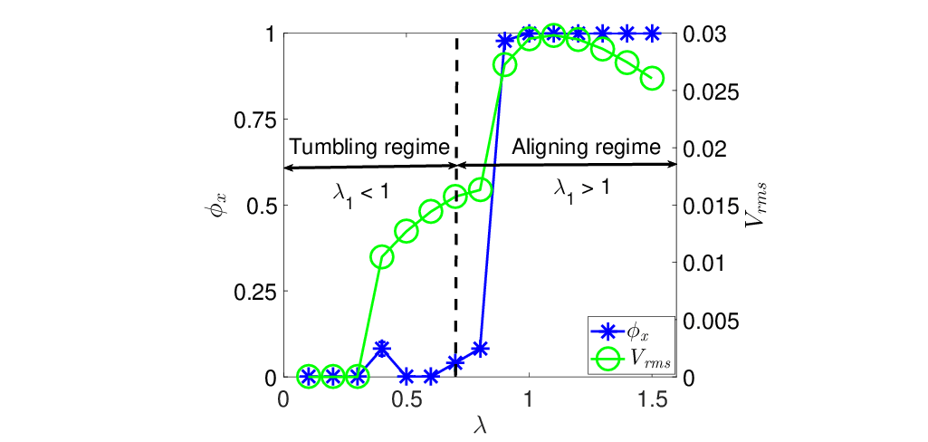
Fig. 1(b) shows the variation of with the flow-aligning parameter for a square channel with . It is evident that increasing results in a sharp crossover from no net flow in the flow-tumbling regime to coherent flow when the fluid becomes flow-aligning. We find that this crossover is robust to changing activity, , orientational elasticity, , and the size of the channel.
We next restrict ourselves to the flow-aligning regime and, guided by the experiments Wu et al. 2017, change the aspect ratio of the channel cross-section. To quantify the aspect ratio we define AR = . For square channels AR, whereas if and differ significantly, AR .
Fig. 1(c) summarises the geometry dependence of the coherent to turbulent flow transition by measuring the flow order parameter, , as a function of the aspect ratio of the channel. Interestingly, there is a sharp transition between coherent flow states and active turbulence as the aspect ratio increases beyond .
To understand this behaviour we use the simulations to more closely examine the details of the flow structure close to the transition from net flow to the active turbulent state. Near the transition point, AR , neither purely laminar flow nor fully-developed turbulent flow are observed. Instead, the active fluid can demonstrate oscillatory flow or a lattice of vortex-rolls. The different flow states observed as the channel size is increased are shown in Fig. 2.
For very narrow channels the active instability is suppressed and there is no flow. An increase in the channel size first leads to active flows that are completely unidirectional, with a velocity vector that only has a component along the channel length, (Fig. 2(a)). For slightly wider channels, the flows can develop an oscillatory component and (Fig. 2(c)). However, the velocity along the channel remains the dominant component of the velocity field with its maximum value near the center line of the channel. Since is dominant in both unidirectional and oscillatory flows, these both manifest as coherent states which result in a net fluid transport through the channel.
Further increases in the size of the channel can, however, lead to flow configurations where the net flow is absent. The vortex-roll state is characterized by three-dimensional, counter-rotating vortices located on a one-dimensional lattice along the length of the channel, as shown in Fig. 2(e). The axes of the vortices invariably lie along the smallest channel dimension ( direction). On any cross-section perpendicular to the direction, the 3D flow appears similar to the dancing flows reported earlier in 2D simulations Shendruk et al. 2017; Chandragiri et al. 2019 and 2D confined microtubule and motor protein mixtures Hardoüin et al. 2019. Regions with appear in the corresponding director field indicating the presence of disclination lines (Fig. 2(f)). These structures are dynamic and may form either in the bulk or near the walls. Finally, in large channels, we recover active turbulence, characterised by a spatio-temporally evolving director field (Figs. 2(g), 2(h)) which results in contortion of disclination lines and their irregular spatial arrangement Shendruk et al. 2018; Binysh et al. 2020; Duclos et al. 2020.
Mechanism:- We can now explain the disappearance of net flow as the aspect ratios of the channels increase. Firstly we note that, as a result of hydrodynamic screening, the vorticity correlation length in the channel, , is set by its smallest dimension, . Evidence for this is presented in Fig. 3(a) where we show that the vorticity correlation length , (measured in the plane at ) tracks until the channel becomes too wide to screen the flows and the correlation length crosses over to its bulk value . For comparison, Fig. 3(b) shows that there is no correlation between and the larger dimension of the channel cross section . However, the structure of the flow is determined by . If , vortices cannot form and there is a net flow. If, however, the larger dimension of the channel cross section becomes available for the flow streamlines to turn, form vortices, and destroy the coherent net flow along the channel. This also explains why the vortex rolls are always ordered along the channel length with their axis along the shortest dimension of the channel. No analytical estimate for the exact value of the coefficient in these inequalities is available. However numerical simulations of 2D confined active nematics Shendruk et al. 2017 suggest that when vortex rolls first form. This corresponds to . Note that the argument breaks down when both and are larger than the bulk correlation length, : active turbulence will then destroy any net flow regardless of the aspect ratio.


Discussion:- Our results demonstrate that, in flow-aligning, 3D, active microfluidics, the emergence of coherent net flow states is controlled by the aspect ratio of the channel cross section: coherent flows are possible in channels with cross sections that are close to isotropic, but are destroyed in channels with larger aspect ratios. This can be explained by whether or not vortex rolls have room to form across the larger cross-section dimension, thus destroying coherent flow. The length scale of the vortices is set by hydrodynamic screening controlled by the smaller dimension.
The aspect-ratio dependence agrees with recent experiments on microtubule-motor protein mixtures in microfluidic channels Wu et al. 2017. However, to more closely compare the results with the experimental system, the model in its current form requires a number of adjustments. First, here we assume a uniform density throughout the channel, while the experiments clearly indicate that layers of concentrated aligned microtubules can build up at the confining boundaries. Indeed, the experimental results were attributed to such surface ordering, but we show here that the aspect ratio induced flow transition does not require wetting of the channel walls by a nematic layer. Second, it is possible that free-slip velocity boundary conditions and weak-planar anchoring of the orientation might result in a more accurate representation of experiments as the microtubules appear to weakly align and slide freely at the boundaries Hardoüin et al. 2019; Opathalage et al. 2019. We also show that the transition relies upon the active fluid being flow-aligning, thus identifying the microtubule - motor protein mixtures as belonging to this class of nematic fluids.
References
- Saw et al. (2017) T. B. Saw, A. Doostmohammadi, V. Nier, L. Kocgozlu, S. Thampi, Y. Toyama, P. Marcq, C. T. Lim, J. M. Yeomans, and B. Ladoux, Nature 544, 212 (2017).
- Duclos et al. (2018) G. Duclos, C. Blanch-Mercader, V. Yashunsky, G. Salbreux, J.-F. Joanny, J. Prost, and P. Silberzan, Nat. Phys. 14, 728 (2018).
- Wensink et al. (2012) H. H. Wensink, J. Dunkel, S. Heidenreich, K. Drescher, R. E. Goldstein, H. Löwen, and J. M. Yeomans, Proc. Natl. Acad. Sci. U.S.A. 109, 14308 (2012).
- Dunkel et al. (2013) J. Dunkel, S. Heidenreich, K. Drescher, H. H. Wensink, M. Bär, and R. E. Goldstein, Phys. Rev. Lett. 110, 228102 (2013).
- Kumar et al. (2014) A. Kumar, A. Maitra, M. Sumit, S. Ramaswamy, and G. Shivashankar, Sci. Rep. 4, 3781 (2014).
- Kruse et al. (2004) K. Kruse, J.-F. Joanny, F. Jülicher, J. Prost, and K. Sekimoto, Phys. Rev. Lett. 92, 078101 (2004).
- Schaller et al. (2010) V. Schaller, C. Weber, C. Semmrich, E. Frey, and A. R. Bausch, Nature 467, 73 (2010).
- Koch and Subramanian (2011) D. L. Koch and G. Subramanian, Annu. Rev. Fluid Mech. 43, 637 (2011).
- Ramaswamy (2010) S. Ramaswamy, Annu. Rev. Condens. Matter Phys. 1, 323 (2010).
- Marchetti et al. (2013) M. C. Marchetti, J.-F. Joanny, S. Ramaswamy, T. B. Liverpool, J. Prost, M. Rao, and R. A. Simha, Rev. Mod. Phys. 85, 1143 (2013).
- Gompper et al. (2020) G. Gompper, R. G. Winkler, T. Speck, A. Solon, C. Nardini, F. Peruani, H. Löwen, R. Golestanian, U. B. Kaupp, L. Alvarez, et al., J. Phys. Condes. Mat. 32, 193001 (2020).
- Bricard et al. (2013) A. Bricard, J.-B. Caussin, N. Desreumaux, O. Dauchot, and D. Bartolo, Nature 503, 95 (2013).
- Wioland et al. (2016) H. Wioland, E. Lushi, and R. E. Goldstein, New J. Phys. 18, 075002 (2016).
- Wu et al. (2017) K.-T. Wu, J. B. Hishamunda, D. T. Chen, S. J. DeCamp, Y.-W. Chang, A. Fernández-Nieves, S. Fraden, and Z. Dogic, Science 355, eaal1979 (2017).
- Conrad and Poling-Skutvik (2018) J. C. Conrad and R. Poling-Skutvik, Annu. Rev. Chem. Biomol. 9, 175 (2018).
- Poujade et al. (2007) M. Poujade, E. Grasland-Mongrain, A. Hertzog, J. Jouanneau, P. Chavrier, B. Ladoux, A. Buguin, and P. Silberzan, Proc. Natl. Acad. Sci. U.S.A. 104, 15988 (2007).
- McLennan et al. (2012) R. McLennan, L. Dyson, K. W. Prather, J. A. Morrison, R. E. Baker, P. K. Maini, and P. M. Kulesa, Development 139, 2935 (2012).
- Clark and Vignjevic (2015) A. G. Clark and D. M. Vignjevic, Curr. Opin. Cell. Biol. 36, 13 (2015).
- Whitesides (2006) G. M. Whitesides, Nature 442, 368 (2006).
- Beebe et al. (2002) D. J. Beebe, G. A. Mensing, and G. M. Walker, Annu. Rev. Biomed. Eng. 4, 261 (2002).
- Nguyen et al. (2019) N.-T. Nguyen, S. T. Wereley, and S. A. M. Shaegh, Fundamentals and applications of microfluidics (Artech house, 2019).
- Laser and Santiago (2004) D. J. Laser and J. G. Santiago, J. Micromech. Microeng. 14, R35 (2004).
- Voituriez et al. (2005) R. Voituriez, J.-F. Joanny, and J. Prost, Europhys. Lett. 70, 404 (2005).
- Sanchez et al. (2012) T. Sanchez, D. T. Chen, S. J. DeCamp, M. Heymann, and Z. Dogic, Nature 491, 431 (2012).
- Opathalage et al. (2019) A. Opathalage, M. M. Norton, M. P. Juniper, B. Langeslay, S. A. Aghvami, S. Fraden, and Z. Dogic, Proc. Natl. Acad. Sci. U.S.A. 116, 4788 (2019).
- Hardoüin et al. (2019) J. Hardoüin, R. Hughes, A. Doostmohammadi, J. Laurent, T. Lopez-Leon, J. M. Yeomans, J. Ignés-Mullol, and F. Sagués, Commun. Phys. 2, 1 (2019).
- Suzuki et al. (2017) K. Suzuki, M. Miyazaki, J. Takagi, T. Itabashi, and S. Ishiwata, Proc. Natl. Acad. Sci. U.S.A. 114, 2922 (2017).
- Shendruk et al. (2017) T. N. Shendruk, A. Doostmohammadi, K. Thijssen, and J. M. Yeomans, Soft Matter 13, 3853 (2017).
- Chandragiri et al. (2019) S. Chandragiri, A. Doostmohammadi, J. M. Yeomans, and S. P. Thampi, Soft Matter 15, 1597 (2019).
- Chen et al. (2018) S. Chen, P. Gao, and T. Gao, J. Fluid. Mech. 835, 393 (2018).
- Shendruk et al. (2018) T. N. Shendruk, K. Thijssen, J. M. Yeomans, and A. Doostmohammadi, Phys. Rev. E 98, 010601 (2018).
- Binysh et al. (2020) J. Binysh, Ž. Kos, S. Čopar, M. Ravnik, and G. P. Alexander, Phys. Rev. Lett. 124, 088001 (2020).
- Duclos et al. (2020) G. Duclos, R. Adkins, D. Banerjee, M. S. Peterson, M. Varghese, I. Kolvin, A. Baskaran, R. A. Pelcovits, T. R. Powers, A. Baskaran, et al., Science 367, 1120 (2020).
- Santhosh et al. (2020) S. Santhosh, M. R. Nejad, A. Doostmohammadi, J. M. Yeomans, and S. P. Thampi, J. Stat. Phys. , 1 (2020).
- Batchelor and Batchelor (2000) C. K. Batchelor and G. Batchelor, An Introduction to Fluid Dynamics, illustrated, reprint ed. (Cambridge University Press, UK, 2000).
- De Gennes and Prost (1995) P.-G. De Gennes and J. Prost, The physics of liquid crystals (Oxford University Press, UK, 1995).
- Giomi et al. (2013) L. Giomi, M. J. Bowick, X. Ma, and M. C. Marchetti, Phys. Rev. Lett. 110, 228101 (2013).
- Marenduzzo et al. (2007) D. Marenduzzo, E. Orlandini, M. Cates, and J. M. Yeomans, Phys. Rev. E 76, 031921 (2007).
- Simha and Ramaswamy (2002) R. A. Simha and S. Ramaswamy, Phys. Rev. Lett. 89, 058101 (2002).
- Doostmohammadi et al. (2017) A. Doostmohammadi, T. N. Shendruk, K. Thijssen, and J. M. Yeomans, Nat. Commun. 8, 15326 (2017).
- Desplat et al. (2001) J.-C. Desplat, I. Pagonabarraga, and P. Bladon, Comput. Phys. Commun. 134, 273 (2001).
- Thampi et al. (2013) S. P. Thampi, R. Golestanian, and J. M. Yeomans, Phys. Rev. Lett. 111, 118101 (2013).