Continual Adaptation for Deep Stereo
Abstract
Depth estimation from stereo images is carried out with unmatched results by convolutional neural networks trained end-to-end to regress dense disparities. Like for most tasks, this is possible if large amounts of labelled samples are available for training, possibly covering the whole data distribution encountered at deployment time. Being such an assumption systematically unmet in real applications, the capacity of adapting to any unseen setting becomes of paramount importance. Purposely, we propose a continual adaptation paradigm for deep stereo networks designed to deal with challenging and ever-changing environments. We design a lightweight and modular architecture, Modularly ADaptive Network (MADNet), and formulate Modular ADaptation algorithms (MAD, MAD++) which permit efficient optimization of independent sub-portions of the entire network. In our paradigm, the learning signals needed to continuously adapt models online can be sourced from self-supervision via right-to-left image warping or from traditional stereo algorithms. With both sources, no other data than the input images being gathered at deployment time are needed. Thus, our network architecture and adaptation algorithms realize the first real-time self-adaptive deep stereo system and pave the way for a new paradigm that can facilitate practical deployment of end-to-end architectures for dense disparity regression.
Index Terms:
Stereo Matching, Deep Learning, Self-supervision, Real-time Adaptation, Continual LearningI Introduction
Estimating dense and accurate depth maps is a key perception step to pursue scene comprehension tasks dealing with navigation and interaction with the environment. Passive, image-based techniques aimed at depth perception compare favourably to active sensors in terms of cost, bulkiness as well as - more often than not- working range and flexibility. Among such techniques, stereo vision [1] is usually the preferred choice, requiring just a pair of synchronized and calibrated cameras to measure depth by triangulation between matching pixels.
Akin to most computer vision problems, in the last years deep learning has entered into solutions for stereo matching, at first replacing certain specific steps of the pipeline by neural networks (e.g., matching cost computation [2]) then rapidly converging toward end-to-end architectures [3, 4]. Although end-to-end networks have established the new state-of-the-art in challenging benchmarks such as KITTI [5, 6], they require a large amount of images labelled with ground-truth disparities, in order to effectively learn how to tackle stereo. As obtaining ground-truth disparities, i.e. depths, for real images is particularly challenging and expensive, computer graphics has became a popular alternative to gather thousands of synthetic images endowed with depth labels for free [3]. Although highly realistic, these images can hardly encompass all the nuisances occurring in the real world, such as, e.g., sensor noise, reflective surfaces and challenging illumination conditions. Thus, due to the domain shift between the training and testing environments [7], deep networks trained by computer-generated imagery suffer from a large loss in accuracy when deployed in the real world. A partial solution to this issue consists in fine-tuning the stereo network on few labelled samples from the real domain. Yet, to obtain such ground-truth labels, costly active sensors (e.g., LIDAR) and manual intervention or post-processing are required [8]. Even more importantly, despite fine-tuning by a few real-images may address the synthetic-to-real domain shift, it cannot take into account the countless diverse environmental conditions that a stereo network meant to be deployed in-the-wild may encounter, such as, in autonomous driving scenarios, urban and countryside roads, tunnels, varying weather and sudden changes of the surroundings.
| \begin{overpic}[images/introduction/left.png] \put(88.0,38.0){$\displaystyle{\color[rgb]{1,1,1}\textbf{(a)}}$} \end{overpic} | \begin{overpic}[images/introduction/none.png]\put(88.0,38.0){$\displaystyle{\color[rgb]{1,1,1}\textbf{(b)}}$} \end{overpic} |
| \begin{overpic}[images/introduction/mad.png] \put(88.0,38.0){$\displaystyle{\color[rgb]{1,1,1}\textbf{(c)}}$} \end{overpic} | \begin{overpic}[images/introduction/mad++.png] \put(88.0,38.0){$\displaystyle{\color[rgb]{1,1,1}\textbf{(d)}}$} \end{overpic} |
In our vision, the only viable approach to practical end-to-end deep stereo deals with departing from the traditional training-validation-testing workflow towards a continual adaptation paradigm, so as to realize neural networks able to adapt promptly to new situations and environments. Of course, this novel paradigm cannot leverage standard supervised learning approaches since ground-truth labels would not be available for any new setting faced in-the-wild.
In this paper we extend our preliminary work on continual adaptation for deep stereo [10], which proposed the first-ever real-time, self-adapting, deep stereo network by relying on self-supervision obtained from the input pair of frames via a photometric loss [11, 12, 13]. Given a sequence of stereo pairs, a straightforward continual adaptation scheme might be realized though the following steps: 1) output the prediction and compute the loss for the current pair of frames; 2) update the whole network by back-propagation; 3) move forward to the next pair of frames, with enriched knowledge encoded in the updated weights. However, due the computational overhead associated with on-line back-propagation, most state-of-the-art stereo architectures would not operate in real-time under a continual adaptation paradigm mandating full update of the network via back-propagation. Thus, we designed a Modularly ADaptive Network (MADNet) architecture that is fast, accurate and features small memory requirements. Moreover, we developed a Modular ADaptation (MAD) algorithm that, in each on-line back-propagation step, enables to select and update only a portion of the whole MADNet, thereby vastly reducing the overhead required by online model updating and permitting prediction alongside self-adaptation in real-time without a large loss in accuracy compared to back-propagating errors into the full set of weights of network.
We extend and improve the MADNet-MAD framework by leveraging on proxy supervision obtained from traditional stereo algorithms [7, 14]. Indeed, although deep stereo networks are unmatched when trained and tested on similar domains, traditional methods, like [15], are largely domain-agnostic. In fact, they behave similarly and suffer from the same nuisances (e.g., low-textured regions, occlusions, repetitive patterns) with both synthetic and real images as well as across diverse environmental settings. This suggests that traditional algorithms may be exploited to supervise online deep stereo networks if matching errors, i.e. outliers, are properly detected and filtered out. We show that this strategy yields a much stronger adaptation ability and that this results consistently in a significant shrink of the performance gap between modular and full adaptation of MADNet, with the former often turning out even more beneficial than the latter. As a matter of fact, Figure 1 shows a qualitative comparison between the MAD formulation described in [10] and the novel approach proposed in this paper, referred to hereinafter as MAD++. Moreover, we dig into our continual adaptation paradigm and thoroughly explore its behaviour across very different datasets, showing, in particular, that our proposal is not affected by catastrophic forgetting while, on the contrary, continually adapting the stereo network is beneficial to performance in case of domain changes.
The main contributions of this unabridged paper on our work on continual adaptation for deep stereo can be summarized as follows.
- •
We introduce MAD++ which ameliorates our MAD framework by leveraging on proxy supervision provided by traditional stereo algorithms. This novel approach outperforms the original proposal and yields often better results than updating all network weights while running twice faster.
- •
We extensively evaluate both MAD and MAD++ on the raw KITTI dataset already considered in [10]. Besides, we include experiments on two additional datasets, i.e. DrivingStereo [9] and WeanHall [16], so as to provide stronger evidence on the effectiveness of our proposed framework in a broader variety of target domains.
- •
We test our methods across datasets to highlight how continual learning is robust to domain shifts. We find no evidence of catastrophic forgetting in any experiments. On the contrary, we show that models adapted elsewhere feature better adaptation ability when facing new domains.
II Related work
In this section, we briefly review the literature relevant to our work.
Machine learning for stereo. The first attempts to use machine learning for stereo matching dealt with estimating confidence measures [17], either by random forest [18, 19, 20, 21] or CNNs [22, 23, 24, 25], and often with the purpose of improving the final accuracy when combined with traditional algorithms. Regarding stereo algorithms, the first works proposed matching cost functions realized by patch-based CNNs [2, 26, 27] and allowed to achieve state-of-the-art performance by replacing handcrafted cost functions [28] within the SGM pipeline [15]. Later, Batsos et al.[29] combined traditional matching functions within a random forest framework to obtain better generalization across domains. Then, Shaked and Wolf [30] proposed to rely on deep learning for matching cost computation, disparity selection and confidence prediction, while Gidaris and Komodakis [31] focused on disparity refinement.
A true paradigm shift did occur with the first end-to-end stereo network, DispNetC, was proposed alongside large synthetic training datasets [3]. In [3] a custom correlation layer was designed to encode the similarities between pixels as features. Kendall et al.[4] designed GC-Net, switching towards 3D networks that build a cost volume by means of features concatenation. These two architectures started the development of two main families of networks, referred to as 2D and 3D, respectively. Proposals belonging to the former class use typically a single or multiple correlation layers [32, 33, 34, 35, 36, 10, 37, 38], while 3D networks build 4D volumes by means of concatenation [39, 40, 41, 42, 43, 44, 45, 46, 47], features difference [48] or group-wise correlations [49], both combined with active sensors such as LIDAR in [50]. Although most works focus on accuracy, others deploy lightweight architectures [10, 42, 48] aimed at real-time performance, sometimes combining stereo with semantic segmentation [51] or pursuing scene flow [52, 53]. Unfortunately, however, all end-to-end stereo networks are prone to domain shift, as performance decay dramatically when the model is run in environments different from those observed at training time, as shown in [7, 14, 54, 10, 55].
Self-supervision from photometric losses. View synthesis has been recently used to train depth estimation networks in a self-supervised manner by photometric losses [12, 56]. For monocular depth estimation, multiple images are deployed at training time in order to replace ground-truth labels by warping the different views, coming either from stereo pairs or image sequences, according to the predicted depth and minimizing the photometric error between real and warped images [57, 56, 12, 58, 59]. Other recent works follow a similar approach for deep stereo matching [11, 13, 60, 61, 62, 10]. Unlike monocular ones, however, in stereo setups the input images used to compute the photometric loss are available at both training and testing time, which renders this self-supervised learning protocol amenable to continual adaptation.
Proxy-supervision from distilled labels. A further approach consists in sourcing pseudo ground-truth annotations, namely proxy labels, accurate enough to allow for effective supervision during training. The process to obtain these annotations is usually referred to as distillation. In the field of depth estimation, the work by Tonioni et al.[7, 14] was the first to use traditional stereo algorithms filtered out by means of confidence measures for offline adaptation of deep stereo networks. Pang et al.[54] used iterative optimization over proxy labels of the network itself obtained at higher resolutions. Recently, these approaches have been applied to monocular depth estimation, sourcing proxies either from traditional stereo algorithms [63], a teacher architecture [64] or the network itself trained in two stages [65].
III Continual Adaptation
State-of-the-art deep stereo networks are severely challenged by Out-of-Distribution generalization, frequently exhibiting large accuracy drops when deployed across different environments. This issue is typically alleviated by fine-tuning the network on additional labelled samples from the target distribution. We argue that this is definitely unpractical as 1) it requires collecting data and tuning the model before real deployment for any target environment and 2) ground-truth labels need to be acquired together with images.
Self-supervision and distillation allow to circumvent the need for ground-truth labels, making offline fine-tuning the main obstacle towards seamless deployment in-the-wild. This can be addressed by moving from a traditional train-validation-test procedure to a continual adaptation paradigm, whereby the distinction between offline training and online testing is relaxed due to both being performed online and at once. In Algo 1 we provide a description of a continual adaptation process referred to as Full Adaptation. Given a stereo network parametrized by a set of weights , at any given time frame we read a new stereo pair , made out of a left and right image , and predict a disparity map for image based on the current set of parameters . Then, a suitable loss function is computed from and used to update the network weights before reading the next stereo pair .
Since a train iteration is performed on-the-fly on each incoming stereo pair, the network always learns and - potentially- improves by gathering knowledge from the sensed environment. It is worth pointing out that this approach is different from standard practice dealing with updating a network on a batch of images to optimize it over a set of variegate samples that better approximate the entire training set and lead to more stable gradients. In our setting, however, the update steps occur on images that are acquired closely in time and are, therefore, very similar. Thus, the gradients provided by the individual samples are quite similar to the average gradient that would be computed in a batch. In the supplementary material we show that updating the network on a batch of samples does not provide significant benefits.
As shown in [10], our straightforward formulation, though intuitive and effective, introduces a non-negligible computational overhead that does increase the network latency dramatically. To address this drawback, we introduce a modular neural network architecture and a learning algorithm, which are designed to work in synergy to achieve effective continual adaptation with a limited computational overhead.
As pointed out, updating the whole network to achieve continual adaptation is time consuming and may hinder applicability to real-word applications calling for tight low-latency requirements. Due to the time required by back-propagation being proportional to the number of network layers to be traversed, we may speed-up the computation by having fewer layers, i.e. fewer weights, to update. Intuitively this is similar to accelerating forward inference by early-stopping the network processing in order to calculate only a subset of the total number of operations [58, 42]. Our work leverages on a similar intuition to speed up online back-propagation, i.e. the main computational overhead introduced by continual adaptation.

We start from the general encoder-decoder architecture illustrated in Figure 2, which can be thought of as an abstraction of the majority of deep networks proposed for stereo matching in the past years. The layers in network can be organized into non-overlapping, but inter-connected, modules according to any arbitrary grouping policy, e.g., the resolution at which they operate, as shown in different colors in the figure. Then, we might think of performing back-propagation on only one module at a time to speed it up. However, standard network architectures provide only a prediction amenable to computing the loss at the very last layer. Therefore to back-propagate the training signal to each module we would still need to go through the deeper ones in the architecture. To overcome this limitation, we introduce shortcut back-propagation routes for each module. Our network predicts as many outputs as the modules, , and includes at least one back-propagation route from each output to all the layers belonging to the associated module, i.e. with . Hence, by computing a loss for each output, we can directly back-propagate into the corresponding module avoiding the remaining ones by means, for instance, of skip connections (depicted as arcs in Figure 2). The gradients computed with this strategy are an approximation of the trues ones, but they do provide a good training signal, as it will be shown experimentally.
An example of such a design is detailed in subsection III-C and used in the experiments reported in this paper. In this architecture each is a disparity prediction at a different spatial resolution, with denoting the highest resolution disparity map delivered as output, while each includes all the network layers processing features at that resolution, i.e., both in the encoder and the decoder. Due to all the layers in being connected through at least a direct back-propagation path, we can approximate the gradients for all layers by back-propagating only through the direct connection and skipping all the other back-propagation routes. This paradigm approximates back-propagation into the whole network by updating layers through time, e.g. in steps should the modules be sequentially updated, while providing a fast inference time, as required by many practical applications.
III-A Modular ADaptation – MAD
To pursue the modular adaptation approach described in the previous section as effectively as possible, we have developed a selection strategy aimed at choosing the module to be updated at each time step. Purposely, we have devised the reward/punishment algorithm outlined in Algo 2. At bootstrap (2), a histogram consisting of bins (one per module) is initialized to zero. Then, at each time step the disparity maps are predicted (6) and the corresponding losses computed (7). Then, we select a network module by sampling an index from the probability distribution associated with (8) and perform back-propagation into only (9). At this point, our network has been updated and it is ready to process the next stereo pair. Before moving on, we also update in order to reward or punish the module updated in the previous time step, namely , depending on whether this has proven to be effective or not. To do so, we linearly extrapolate the expected value for the highest resolution loss (i.e., that computed on the final output of the network), , from the previous ones at times and (13). Then, we compute the difference, , between the expected and computed losses (14). In case of a positive/negative difference we deem the update step on the module selected at time to have been effective/ineffective as at time the highest resolution loss turns out smaller/larger than the value we would have expected had module not been updated. Accordingly, we gradually apply a decay factor to all entries in (15) , then we reward/punish module by adding a contribution into histogram bin (16). In our experiments, we set and to 0.99 and 0.01, respectively, and in the supplementary material we show how the sensitivity of the algorithm to these parameters is moderate.
In [10] we realized Algo 2 using as , the self-supervised loss provided by the photometric error between the left image and the right image warped according to the estimated disparity . In particular, according to a popular choice in literature, we compute this photometric error as
| (1) |
with set to 0.85 [12]. Thus the approach refereed to as MAD) in this paper performs real-time continual adaptation by deploying a popular self-supervised loss within Algo 2. Although fast and effective, MAD consists in diluting over time the network optimization process, thereby requiring more frames (i.e., update steps) than the straightforward full adaptation approach (Algo 1) to acquire the knowledge needed to adapt a model to a novel environment. In the next section we describe how to leverage on a different kind of loss which deploys a stronger source of supervision while still being amenable to continual adaptation. In section IV we will show how this novel formulation can effectively accelerate a network optimization process distributed over time according to Algo 2 and reduce the performance gap with respect to Algo 1 dramatically.
III-B Proxy-Supervised Modular ADaptation – MAD++
To speed-up the model adaptation process, we move toward a stronger form of supervision. In particular, we propose to rely on proxy supervision by leveraging on a reliable external source of disparities used as proxies for ground-truth labels. For instance, the use of active sensors, like LIDARs, have been proposed to supervise a depth prediction network [66]. Yet, a cheaper - and far more practical- source of proxy labels is described in recent works concerning both stereo [7, 14] and monocular [63] depth estimation. Accordingly, the noisy disparities computed by traditional stereo algorithms are filtered by a confidence estimator and deployed as proxy ground-truth labels to either adapt or train from scratch a depth prediction model. Since the procedure described in Algo 2 is agnostic to the actual loss function, we can extend our modular adaptation approach so as to rely on proxy supervision by simply specifying a suitable loss . This novel formulation of Algo 2 will be referred to hereinafter as MAD++.
Given a generic stereo matching pipeline , we can obtain a noisy disparity map by processing an input stereo pair . However, as discussed in [7, 14], to effectively supervise a depth estimation network it is crucial to filter out most of the noisy disparities. This can be achieved by estimating a confidence map, , encoding the reliability of each pixel in [7, 14]. Then, supervision for any estimated can be obtained from by the following loss function:
| (2) |
where denotes an indicator function that selects the measurements in characterized by a sufficiently high confidence, e.g.a threshold operator applied to each pixel according to the estimated confidence :
| (3) |
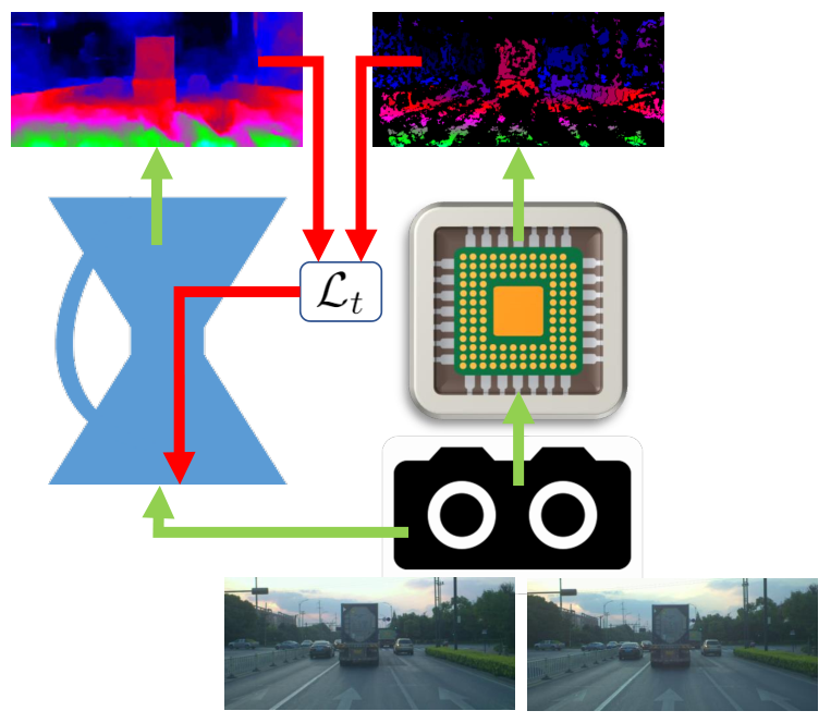
Stereo Matching. Proxy labels can be obtained from an external stereo algorithm with a negligible overhead compared to the computational complexity of a deep stereo network. Indeed, a number of stereo cameras endowed with on-board processing hardware designed to deliver disparity maps at 50+ FPS are available nowadays [67, 68, 69, 70, 71, 72, 73]. As these cameras do not offload the stereo matching computation to the host device, they are amenable to distilling knowledge, i.e. proxy ground-truth disparities, to a deep stereo network so as to run continual adaptation without slowing down the process. Figure 3 illustrates how a stereo camera equipped with on-board processing can be deployed to support our real-time continual adaptation framework for deep stereo.
Due to existing hardware platforms relying mainly on the Semi-Global Matching (SGM) [15] or the basic Block Matching stereo algorithms, we will consider these two options in order to distill proxy disparities within MAD++.
Proxy Filtering. As traditional stereo matchers deliver noisy disparity maps, an effective criterion, in Equation 3, is necessary to filter out outliers and provide reliable supervision to the continual adaptation process. In [7, 14] confidence estimation came from a large neural network, which, in our framework, would add a substantial computational overhead and prevent continual adaptation in real-time. Thus, in MAD++ we pursue a different approach and rely on computationally efficient strategies geared toward the adopted stereo algorithm. Following [74], we deploy a simple left-right check for SGM and a combination of six confidence measures proposed in [75] for Block Matching. From now on, the two settings will be dubbed as SGM and WILD.
In Figure 4 we show qualitative examples of proxies obtained with the aforementioned pipelines on the DrivingStereo dataset [9]. We point out that both succeed in providing reliable proxy labels only, as required by the framework set forth in [7, 14], with density depending on the accuracy of the actual stereo matcher.
| \begin{overpic}[images/proxies/left.png] \put(2.0,38.0){$\displaystyle{\color[rgb]{1,1,1}\textbf{(a)}}$} \end{overpic} | \begin{overpic}[images/proxies/gt.png] \put(2.0,38.0){$\displaystyle{\color[rgb]{1,1,1}\textbf{(b)}}$} \end{overpic} |
| \begin{overpic}[images/proxies/wild_raw.png] \put(2.0,38.0){$\displaystyle{\color[rgb]{1,1,1}\textbf{(c)}}$} \end{overpic} | \begin{overpic}[images/proxies/wild.png] \put(2.0,38.0){$\displaystyle{\color[rgb]{1,1,1}\textbf{(d)}}$} \end{overpic} |
| \begin{overpic}[images/proxies/sgm_raw.png] \put(2.0,38.0){$\displaystyle{\color[rgb]{1,1,1}\textbf{(e)}}$} \end{overpic} | \begin{overpic}[images/proxies/sgm.png] \put(2.0,38.0){$\displaystyle{\color[rgb]{1,1,1}\textbf{(f)}}$} \end{overpic} |
| Layer | Kernel | Stride | Dilate | Output Channels | Input/Output Resolution | Input |
| Encoder | ||||||
| f_conv1_a | 3 | 2 | 1 | 16 | input | |
| f_conv1_b | 3 | 1 | 1 | 16 | f_conv1_a | |
| f_conv2_a | 3 | 2 | 1 | 32 | f_conv1_b | |
| f_conv2_b | 3 | 1 | 1 | 32 | f_conv2_a | |
| f_conv3_a | 3 | 2 | 1 | 64 | f_conv2_b | |
| f_conv3_b | 3 | 1 | 1 | 64 | f_conv3_a | |
| f_conv4_a | 3 | 2 | 1 | 96 | f_conv3_b | |
| f_conv4_b | 3 | 1 | 1 | 96 | f_conv4_a | |
| f_conv5_a | 3 | 2 | 1 | 128 | f_conv4_b | |
| f_conv5_b | 3 | 1 | 1 | 128 | f_conv5_a | |
| f_conv6_a | 3 | 2 | 1 | 192 | f_conv5_b | |
| f_conv6_b | 3 | 1 | 1 | 192 | f_conv6_a | |
| Decoder | ||||||
| d_conv1 | 3 | 1 | 1 | 128 | 1 | input |
| d_conv2 | 3 | 1 | 1 | 128 | 1 | d_conv1 |
| d_conv3 | 3 | 1 | 1 | 96 | 1 | d_conv2 |
| d_conv4 | 3 | 1 | 1 | 64 | 1 | d_conv3 |
| d_conv5 | 3 | 1 | 1 | 32 | 1 | d_conv4 |
| y | 3 | 1 | 1 | 1 | 1 | d_conv5 |
| Refinement | ||||||
| r_conv1 | 3 | 1 | 1 | 128 | 1 | input |
| r_conv2 | 3 | 1 | 2 | 128 | 1 | r_conv1 |
| r_conv3 | 3 | 1 | 4 | 128 | 1 | r_conv2 |
| r_conv4 | 3 | 1 | 8 | 64 | 1 | r_conv3 |
| r_conv5 | 3 | 1 | 16 | 32 | 1 | r_conv4 |
| r_conv6 | 3 | 1 | 1 | 1 | 1 | r_conv5 |
III-C Modularly ADaptive Network – MADNet
In this section we detail the network architecture designed following the abstraction depicted in Figure 2 and deployed throughout the experimental evaluation presented in section IV. Besides the requirements set forth by modular adaptation (Algo 2), we have developed Modularly ADaptive Network (MADNet) to achieve a good balance between speed and accuracy. Indeed, MADNet has a smaller memory footprint and delivers disparity maps much more rapidly with a small loss in accuracy compared to complex networks such as [4, 39, 33]. To design (MADNet) we took inspiration from recent architectures for optical flow [76, 77] and conceived a novel light-weight model for stereo depth estimation.
We pursue dense disparity regression by a pyramidal approach amenable to modularize the architecture and conducive to fast processing. Following Figure 2, our network estimates disparities , with , ranging from to resolution, respectively. As for the encoding section, we design two pyramidal features extractors with shared weights that process the left and right image through a cascade of blocks, as detailed in Table I (Encoder). Based on the lowest resolution feature maps, a correlation layer [3] computes raw matching costs between the left and right images. Then, we deploy a disparity decoder, detailed in Table I (Decoder), predicting the disparity prediction at the lowest resolution, i.e. .
The lowest resolution disparity map is up-sampled by bilinear interpolation to 2 the resolution and used to warp the right features towards the left ones, with both feature maps then forwarded to a further correlation layer and another disparity Decoder in order to estimate . Again, this map is up-sampled to the next resolution level and the same computation as in the previous level is carried in order to come up with disparity estimate . This scheme is repeated until estimate is reached. The warping mechanism is instrumental to use a small search range at any resolution level, i.e. , that is equivalent, at the lowest scale, to a search range of 128, to which a further 2i range is added at each up-sampling. The highest resolution disparity estimate, , is further processed by a refinement module [77], as detailed in Table I (Refinement). Finally, the refined is up-sampled from to full resolution by bilinear interpolation.
| LEAStereo | CSPN | GANet | AcfNet | HD3 | DeepPruner | GWCNet | Bi3D | AANet | DispNetC | MADNet | StereoNet | |||
|---|---|---|---|---|---|---|---|---|---|---|---|---|---|---|
| [46] | [45] | [43] | [44] | [37] | [38] | [49] | [78] | [47] | [3] | [10] | [48] | |||
| D1-all | 1.65 | 1.74 | 1.81 | 1.89 | 2.02 | 2.15 | 2.11 | 2.21 | … | 2.55 | 4.34 | 4.66 | 4.83 | |
| Time† | 0.30 | 1.00 | 1.80 | 0.18 | 0.48 | 0.14 | 0.32 | 0.48 | 0.06 | 0.06 | 0.02 | 0.02 | ||
With reference to Figure 2, in MADNet a generic module consists of a block from the encoding section together with the corresponding disparity decoder, with the arcs linking together the encoder and decoder within a module realized by the warping and correlation layers. Yet, due to being at quarter resolution, is slightly different: in includes the first two of the six encoding blocks alongside both the disparity decoder and the refinement network.
IV Experimental results
In this section, we wish to evaluate thoroughly the effectiveness of our continual adaptation framework. Purposely, we run a set of experiments on a variegated family of datasets.
| City (8027 frames) | Residential (28067 frames) | Campus (1149 frames) | Road (5674 frames) | |||||||
| Starting Model | Adapt. Mode | Proxy src. | D1-all(%) | EPE | D1-all(%) | EPE | D1-all(%) | EPE | D1-all(%) | EPE |
| MADNet | No | ✗ | 37.42 | 9.96 | 37.04 | 11.34 | 51.98 | 11.94 | 47.45 | 15.71 |
| MADNet | FULL | ✗ | 3.35 | 1.11 | 2.38 | 0.94 | 10.62 | 1.78 | 2.72 | 1.04 |
| MADNet | MAD | ✗ | 7.51 | 1.63 | 4.37 | 1.32 | 22.27 | 3.66 | 9.38 | 2.04 |
| (+4.16) | (+0.52) | (+1.99) | (+0.37) | (+11.65) | (+1.88) | (+6.66) | (+1.00) | |||
| MADNet | FULL++ | SGM [15] | 3.51 | 1.12 | 2.27 | 0.94 | 9.69 | 1.63 | 3.18 | 1.05 |
| MADNet | MAD++ | SGM [15] | 4.12 | 1.18 | 3.31 | 1.04 | 11.24 | 1.76 | 5.32 | 1.22 |
| (+0.62) | (+0.06) | (+1.04) | (+0.10) | (+1.55) | (+0.13) | (+2.14) | (+0.17) | |||
| MADNet | FULL++ | WILD [75] | 5.11 | 1.23 | 2.82 | 0.99 | 11.79 | 1.89 | 4.28 | 1.11 |
| MADNet | MAD++ | WILD [75] | 5.75 | 1.30 | 2.88 | 0.99 | 13.93 | 2.04 | 5.39 | 1.24 |
| (+0.65) | (+0.07) | (+0.06) | (-0.01) | (+2.13) | (+0.15) | (+1.11) | (+0.13) | |||
IV-A Datasets
Here, we provide a description of the datasets used for the experiments.
FlyingThings3D. A collection of synthetic images, made out of about 22k training stereo pairs with dense ground-truth labels, part of the SceneFlow synthetic dataset [3]. This dataset has been used to pre-train MADNet before deployment on real images, according to the standard practice in recent deep stereo literature outlined in [10]. Specifically, we perform 1.2M training iterations using Adam Optimizer and a learning rate of 10-4, halved after 400K steps and further every 200K until convergence. As loss function, we compute the L1 difference between disparity maps estimated at each resolution and downsampled ground-truth labels. The final loss is a weighted sum of the contributions from the different resolutions, with weights set to 0.005, 0.01, 0.02, 0.08, 0.32 from to according to [77].
KITTI 2015 train set. A collection 200 stereo pairs with sparse ground-truth maps, obtained from post-processed LIDAR measurements and 3D CAD objects [6]. This dataset has been used to fine-tune MADNet for 500K steps with learning rate by computing the loss only on the full-resolution disparity map and using 0.001 as weight, as described in [10]. From now on, a MADNet model trained on FlyingThings3D and fine-tuned on KITTI 2015 with explicit supervision will be referred to as MADNet-GT.
Raw KITTI. A large dataset featuring 61 stereo sequences, for a total of about 43k pairs with different image resolution. We use a constant resolution of pixels by taking central crops of the original frames [10]. As depth ground-truths, we use filtered LIDAR measurements [8] converted to disparities through known calibration parameters [10]. According to the classification reported in the official website, we group sequences into four main categories: Road, Residential, Campus and City. Then, we concatenate the sequences belonging to the same category so as to obtain new, longer sequences of 5674, 28067, 114911 1 About Campus, it represents the most challenging environment characterized by low-textured buildings, yet the shortest sequence. For this reason, we loop twice over the sequence as in [10]. and 8027 frames for the above mentioned categories, respectively. In this manner, we simulate four macro environments characterised by different peculiarities, i.e. City and Residential mostly show roads surrounded by buildings, while Road images are collected while driving in highways and country roads, thus mainly depicting cars and vegetation. The dataset provides also raw LIDAR measurements.
DrivingStereo. A recent dataset [9] collecting about 170k stereo images grouped in 38 sequences with average resolution of pixels. ground-truth is obtained by iterative filtering of LIDAR labels by means of a stereo CNN. We select three challenging sequences, namely 2018-08-17-09-45, 2018-10-11-17-08 and 2018-10-15-11-43, consisting of 1667, 1119 and 4950 frames, respectively. We rename the above mentioned sequences as Rainy, Cloudy and Country, respectively, according to their main peculiarities, We selected these sequences to 1) evaluate short-term adaptation (i.e., after few hundreds frames) in challenging conditions (e.g., rainy) and 2) assess the impact of prior continual adaptation (e.g., on KITTI) when moving to a new environment.
WeanHall. An indoor dataset [16] which includes 6510 stereo pairs. As the working environment is very different from the autonomous driving scenarios addressed by previous datasets, we deem it worth evaluating performance also when continually adapting MADNet in so diverse settings. Unfortunately, no ground-truth disparities/depths are provided in WeanHall, neither are we aware of any other indoor stereo dataset providing sequences of real images alongside with the corresponding ground-truth labels. Therefore, we rely on the photometric error (Equation 1) to provide quantitative performace figures on WeanHall.
IV-B Experimental protocol
To assess the performance of our continual adaptation schemes, we run disparity prediction on the stereo pairs of a given sequence according to their order, i.e. as if they were acquired online in the field. On KITTI and DrivingStereo we measure the D1-all error rate as the percentage of pixels having absolute disparity error larger than 3 and relative error larger than 5%, as well as the End-Point-Error (EPE), whilst on WeanHall we measure the photometric error upon reprojection, as detailed in Equation 1. In case of baseline performance dealing with prediction without adaptation, we simply compute error metrics for each stereo frame and average them across the entire sequence. In case of adaptation, we process stereo pair to predict a disparity map and compute the error metrics on it, then we update the network according to either Algo 1 (FULL) or Algo 2 (i.e.MAD or MAD++). As a consequence, the impact of the continual adaptation step at time will affect the error metrics from time . Akin to baseline performance, per-sequence metrics are computed by averaging across frames those dealing with the per-frame predictions . During adaptation, we use a momentum optimizer, with a constant learning rate of 10-4 and a momentum of 0.9. Different optimizers or learning rate schedules resulted in minor fluctuations in our experiments. All experiments have been carried out using the source code and trained models available at github.com/CVLAB-Unibo/Real-time-self-adaptive-deep-stereo.
IV-C Comparison with state-of-the-art stereo networks
We start by comparing MADNet to the current state-of-the-art networks on the standard KITTI 2015 benchmark setting, i.e. without performing online adaptation. Table II collects performance figures retrieved from the online benchmark (to which we refer the reader for a complete overview) for both accuracy and runtime, although the latter is measured on GPUs belonging to different hardware generations. We can notice that the most accurate architectures trade precision for speed, whereas MADNet can operate in real-time with a modest increase of the error rate (about 3% with respect to the top-performing network). The focus of our work concern deployingMADNet alongside suitable online adaptation strategies to maximize accuracy while running in real-time in unknown environments.
IV-D Evaluation on KITTI
We begin our evaluation by studying different aspects of continual adaptation on the KITTI dataset. First, we address short-term adaptation within a domain by considering the KITTI sequences belonging to the same category independently. Then, we tackle a setup dealing with long-term adaptation across domains by concatenating together the sequences belonging to the different categories. We report results obtained by both the continual adaptation schemes discussed in section III, namely full adaptation (Algo 1) and the more efficient - though approximated- modular adaptation approach (Algo 2). We also assess upon steering both adaptation schemes by either self-supervision of proxy supervision. As for the latter source of supervision, we consider proxy labels yielded by the previously described SGM and WILD pipelines. As in KITTI raw LIDAR measurements are available alongside stereo pairs, we also investigate on the effectiveness of this form of proxy supervision. Finally, we dig deeper into our framework by analysing the distribution of the update steps across the modules in modular adaptation (Algo 2 and investigating on the computational savings that may be achieved by employing slower adaptation rates.
| Starting Model | Adapt. Mode | Proxy src. | D1-all(%) | EPE |
|---|---|---|---|---|
| MADNet | No | ✗ | 38.84 | 11.68 |
| MADNet | FULL | ✗ | 2.43 | 0.95 |
| MADNet | MAD | ✗ | 4.09 | 1.19 |
| (+1.66) | (+0.24) | |||
| MADNet | FULL++ | SGM [15] | 2.28 | 0.95 |
| MADNet | MAD++ | SGM [15] | 2.46 | 0.98 |
| (+0.18) | (+0.03) | |||
| MADNet | FULL++ | WILD [75] | 2.64 | 0.98 |
| MADNet | MAD++ | WILD [75] | 2.44 | 0.96 |
| (-0.20) | (-0.02) |
| \begin{overpic}[images/density/left.png] \put(1.0,2.0){$\displaystyle{\color[rgb]{1,1,1}\textbf{(a)}}$} \end{overpic} |  |
|---|---|
| \begin{overpic}[images/density/sgm.png] \put(1.0,2.0){$\displaystyle{\color[rgb]{1,1,1}\textbf{(b)}}$} \end{overpic} |  |
| \begin{overpic}[images/density/wild.png] \put(1.0,2.0){$\displaystyle{\color[rgb]{1,1,1}\textbf{(c)}}$} \end{overpic} |  |
| Starting Model | Adapt. Mode | D1-all(%) | EPE |
|---|---|---|---|
| MADNet-Synthia | FULL (baseline) | 2.76 | 1.03 |
| MADNet-Synthia-FOL2A [55] | FULL | 2.60 | 1.01 |
| MADNet-Synthia | FULL++ (ours) | 2.23 | 0.95 |
Online adaptation in-the-wild. We address here the reference scenario concerning practical deployment in-the-wild: a stereo network pre-trained on synthetic data is run in a wholly unknown environment. In this setting, the experimental results reported in Table III and Table IV deals with adaptation within a single domain and across different domains, respectively, both tables following the same organization. The first row highlights the baseline performance measured by pre-training MADNet on FlyingThings3D and then running the model without any kind of online adaptation. Then, we report the results achieved by the two online adaptation schemes, i.e. FULL (Algo 1) and MAD (Algo 2), realized by self-supervision through the photometric error loss, as formulated in our previous work [10]. The next rows concern the novel formulation described in this paper, which exploits different sources of proxy supervision, namely SGM and WILD. Again, FULL++ and MAD++ refer to Algo 1 and Algo 2, respectively. For each source of supervision, we report in blue the difference in terms of D1-all and EPE between the MAD and FULL adaptation schemes, so as to highlight the gap between modular and full adaptation when relying on the same form of supervision. The difference between the two Tables deals with the KITTI sequences belonging to the same category having been processed individually in Table III, after concatenation according to the order Campus City Residential Road, in Table IV.
| City (8027 frames) | Residential (28067 frames) | Campus (1149 frames) | Road (5674 frames) | |||||||
| Starting Model | Adapt. Mode | Proxy src. | D1-all(%) | EPE | D1-all(%) | EPE | D1-all(%) | EPE | D1-all(%) | EPE |
| MADNet-GT | No | ✗ | 2.08 | 0.80 | 2.55 | 0.91 | 6.51 | 1.31 | 1.63 | 0.83 |
| MADNet-GT | FULL | ✗ | 1.60 | 0.89 | 1.87 | 0.86 | 4.70 | 1.31 | 1.14 | 0.81 |
| MADNet-GT | MAD | ✗ | 1.62 | 0.90 | 1.54 | 0.85 | 4.81 | 1.28 | 1.28 | 0.84 |
| (+0.02) | (+0.01) | (-0.33) | (-0.01) | (+0.10) | (-0.03) | (+0.14) | (+0.03) | |||
| MADNet-GT | FULL++ | SGM [15] | 1.59 | 0.92 | 1.49 | 0.84 | 3.50 | 1.05 | 1.24 | 0.85 |
| MADNet-GT | MAD++ | SGM [15] | 1.59 | 0.92 | 1.52 | 0.86 | 3.73 | 1.14 | 1.35 | 0.86 |
| (-0.01) | (0.00) | (+0.03) | (+0.02) | (+0.22) | (+0.09) | (+0.11) | (+0.01) | |||
| MADNet-GT | FULL++ | WILD [75] | 1.58 | 0.90 | 1.50 | 0.85 | 4.19 | 1.13 | 1.24 | 0.83 |
| MADNet-GT | MAD++ | WILD [75] | 1.57 | 0.91 | 1.79 | 0.87 | 4.26 | 1.23 | 1.30 | 0.85 |
| (-0.01) | (+0.01) | (+0.29) | (+0.02) | (+0.07) | (+0.10) | (+0.06) | (+0.02) | |||
| Starting Model | Adapt. Mode | Proxy src. | D1-all(%) | EPE |
|---|---|---|---|---|
| MADNet-GT | No | ✗ | 2.45 | 0.89 |
| MADNet-GT | FULL | ✗ | 1.83 | 0.88 |
| MADNet-GT | MAD | ✗ | 1.94 | 0.86 |
| (+0.11) | (-0.01) | |||
| MADNet-GT | FULL++ | SGM [15] | 1.46 | 0.85 |
| MADNet-GT | MAD++ | SGM [15] | 1.76 | 0.89 |
| (+0.30) | (+0.03) | |||
| MADNet-GT | FULL++ | WILD [75] | 1.48 | 0.85 |
| MADNet-GT | MAD++ | WILD [75] | 1.64 | 0.86 |
| (+0.16) | (+0.01) |
Firstly, the comparison between the baseline performance reported in the first row of both Tables and the figures in the successive ones highlights the dramatic error drops yielded by all considered methods and vouches for the utmost effectiveness of adapting online a stereo model pre-trained on synthetic data and run in a wholly unknown environment. As expected, between the two schemes, full adaptation (FULL/FULL++) consistently outperforms modular adaptation (MAD/MAD++) when steered by the same kind of supervision. Then, as for the former scheme, self-supervision (FULL) and proxy supervision (FULL++) seem, overall, rather equivalent options, one or the other performing slightly better in some experiments: e.g., in Table III FULL provides the lowest D1-all error in City and Road, FULL++(SGM) in Residential and Campus, whereas in Table IV FULL++(SGM) yields smaller errors than FULL which, in turn, outperforms FULL++(WILD).
However, when dealing with modular adaptation, proxy supervision (MAD++) consistently outperforms self-supervision (MAD), often by a very large margin. Indeed, unlike self-supervision, proxy supervision allows for reducing the performance gap between full and modular adaptation dramatically, as highlighted by the figures reported in blue in Table III. We also point out that this is particularly evident in short sequences, such as Campus in Table III, for which the gap is reduced from about 11.83% to less than 3%. Indeed, as shown in Figure 5, MAD++ is much faster than MAD in reaching the same accuracy level as FULL/FULL++, which suggests performance differences measured by error metrics averaged along a sequence likely showing up more evidently in shorter ones. Similar to Table III, proxy supervision turns out particularly beneficial to improve modular adaptation with respect to the formulation based on self-supervision in the long-term, cross-domain adaptation experiments considered in Table IV, with MAD++ turning out almost as effective as FULL++ while observing a substantial gap between MAD and FULL.
When it comes to reasoning on the different proxy sources adopted with either FULL++ or MAD++, we can notice that, more often than not, SGM delivers a more effective supervision than WILD. In fact, the latter provides better performance only with MAD++ in the Residential domain (Table III) and, though rather slightly, in case of cross-domain adaptation ((Table IV). We ascribe this to the much higher density of proxy labels featured by the SGM pipeline compared to WILD, as illustrated qualitatively in Figure 6.
| City (8027 frames) | Residential (28067 frames) | Campus (1149 frames) | Road (5674 frames) | |||||||
| Starting Model | Adapt. Mode | Proxy src. | D1-all(%) | EPE | D1-all(%) | EPE | D1-all(%) | EPE | D1-all(%) | EPE |
| MADNet | No | ✗ | 37.42 | 9.96 | 37.04 | 11.34 | 51.98 | 11.94 | 47.45 | 15.71 |
| MADNet | FULL++ | LIDAR | 3.66 | 0.97 | 2.94 | 0.89 | 9.10 | 1.54 | 3.24 | 0.93 |
| MADNet | MAD++ | LIDAR | 4.63 | 1.12 | 3.99 | 1.06 | 19.33 | 2.32 | 4.74 | 1.12 |
| (+0.97) | (+0.15) | (+1.05) | (+0.18) | (+10.23) | (+0.78) | (+1.50) | (+0.20) | |||
| MADNet-GT | No | ✗ | 2.08 | 0.80 | 2.55 | 0.91 | 6.51 | 1.31 | 1.63 | 0.83 |
| MADNet-GT | FULL++ | LIDAR | 2.00 | 0.67 | 2.17 | 0.75 | 4.29 | 0.96 | 1.59 | 0.66 |
| MADNet-GT | MAD++ | LIDAR | 3.16 | 0.88 | 2.86 | 0.92 | 4.96 | 1.20 | 1.89 | 0.79 |
| (+1.15) | (+0.21) | (+0.69) | (+0.17) | (+0.67) | (+0.23) | (+0.30) | (+0.14) | |||
| Starting Model | Adapt. Mode | Proxy src. | D1-all(%) | EPE |
|---|---|---|---|---|
| MADNet | No | ✗ | 38.84 | 11.68 |
| MADNet | FULL++ | LIDAR | 2.87 | 0.87 |
| MADNet | MAD++ | LIDAR | 3.86 | 1.02 |
| (+0.99) | (+0.15) | |||
| MADNet-GT | No | ✗ | 2.45 | 0.89 |
| MADNet-GT | FULL++ | LIDAR | 2.06 | 0.73 |
| MADNet-GT | MAD++ | LIDAR | 2.86 | 0.89 |
| (+0.81) | (+0.16) |
Proxy supervision vs meta-learning. We compare proxy supervision to the meta-learning framework proposed in [55]. Purposely, according to the setting suggested in [55], we take the MADNet model trained on FlyingThings3D and 1) fine-tune it on Synthia in a traditional, supervised manner or 2) using the First Order approximation variant of L2A (FOL2A). Thus, for this experiment, 1) provides the baseline with respect to which we evaluate the adaptation performance provided by FOL2A and our proposed approach dealing with proxy labels gathered by SGM. In both cases, we use a learning rate of 10-5 and a batch size of 16 for 10K steps. For meta-learning optimization we choose FOL2A [55], since all other strategies resulted unstable when coupled with MADNet, and use 3 consecutive frames. Table V collects the outcome of this experiment. We can notice how using L2A during pre-training can improve the performance with respect to the baseline. However, our proposal turns out significantly more effective, i.e.proxy supervision is more effective than L2A pre-training. A thorough comparison dealing with all the individual sequences is reported in the supplementary material.
Online adaptation after fine-tuning. As proposed in [10], we also investigate on the effectiveness of the different on-line adaptation schemes in case the pre-trained model may be fine-tuned by real stereo pairs with ground-truths before running inference. Indeed, this is the case of some research datasets like KITTI.
Thus, in Table VI and Table VII we report the results dealing with adaptation on each of the four KITTI domains and across domains, the only difference with respect to Table III, Table IV being that now MADNet has been pre-trained on FlyingThings3D and then fine-tuned on the KITTI 2015 training set before undergoing online adaptation by the considered schemes and forms of supervision.
The first row in Table VI and Table VII show the baseline performance yielded by running the pre-trained and fine-tuned model with online adaptation turned off. As now the network has been fine-tuned by samples endowed with ground-truth disparities, the baseline model performs considerably better than in Table III and Table IV. Nevertheless, both full adaptation (FULL/FULL++) as well as modular adaptation (MAD/MAD++) allow to further improve over this strong baseline in all the considered experiments, typically yielding substantial relative performance gains. For instance, in Table VI, FULL++(SGM) and MAD++(SGM) can provide a relative D1-all error reduction of about 46% and 42% on Campus (the shortest sequence), whereas FULL can decrease such error by about 30% in Road and MAD++(WILD) by about 24% in City. Similarly, in Table VII, the relative D1-all error reduction ranges from about 20% (MAD) to as much as 40% (FULL++(SGM)).
Besides, due to the base model undergoing adaptation being stronger, full and modular adaptation tend to exhibit a much smaller gap when driven by the same form of supervision (figures in blue). Moreover, unlike the previous experiment, in most cases proxy supervision provides better performance than self-supervision non only with modular adaptation (MAD++ vs. MAD) but also with full adaptation (FULL++ vs FULL).
As for the two kinds of proxy labels, the WILD pipeline seems now competitive with respect to SGM, as it can provide better or equivalent performance also in case of full adaptation (City and Road in Table VI) and turns out generally more effective when the model undergoes modular adaptation, in particular in the long-term, cross-domain experiment (Table VII). We would be led to ascribe this finding to the fact that, although fewer in number, the proxies extracted by WILD are more accurate and thus more amenable to refine the already good disparities predicted by a strong base model fine-tuned by real images equipped with ground-truths. Conversely, as observed in the previous experiment, denser proxies seem instrumental to break down the gross errors spread throughout the image delivered by a baseline prone to the synthetic-to-real domain shift.
Proxy supervision by LIDAR. We also inquire about the effectiveness of continual adaptation in case proxy supervision may be obtained from raw measurements provided by a LIDAR sensor, as it is the case of the KITTI dataset. Akin to previous experiments, we consider both a baseline MADNet pre-trained on FlyingThings3D as well as a model further fine-tuned by labelled stereo pairs from the KITTI 2015 training set (MADNet-GT). Table VIII and Table IX collect the results dealing with online adaptation on each of the four KITTI domains and across them, respectively. We can notice a trend similar to previous experiments relatively to several key findings. Indeed, in the in-the-wild scenario, online adaptation does matter a lot as in both Tables we observe a dramatic reduction of errors compared to the baseline model pre-trained on synthetic imagery. Besides, FULL++ consistently outperform MAD++, the margin turning out generally higher than with proxy supervision by SGM and WILD (Table III and Table IV). In case stereo pairs with ground-truth are available to fine-tune the pre-trained model, online adaptation by LIDAR proxies and full adaptation (FULL++) is still beneficial, whilst modular adaptation (MAD++) tend to perform worse than the baseline. Hence, we are lead to conclude that modular adaptation (Algo 2) with supervision by LIDAR is less effective than in case the proxy labels are gathered by the SGM and WILD pipeline.
| \begin{overpic}[images/density/left.png] \put(1.0,2.0){$\displaystyle{\color[rgb]{1,1,1}\textbf{(a)}}$} \end{overpic} | |
|---|---|
| \begin{overpic}[images/density/lidar.png] \put(1.0,2.0){$\displaystyle{\color[rgb]{1,1,1}\textbf{(b)}}$} \end{overpic} |  |
Moreover, by comparing Table VIII and Table IX to Tables 1-4, we can notice that, in general, both MADNet and MADNet-GT exhibit a lower EPE when steered by LIDAR supervision thanks to the higher depth resolution provided by the sensor. Yet, the D1-all error tends to be higher. We ascribe this to raw LIDAR measurements featuring a larger number of outliers compared to SGM and WILD because both the latter pipelines include a filtering step to disregard low-confidence disparities. In particular, it is worth observing how raw LIDAR measurements often yield gross errors near depth discontinuities, as illustrated in Figure 7.
Complementing low-density supervision. As shown in both Figure 6 and Figure 7, we can notice how different the density of the labels is by changing the source, with WILD, in particular, resulting the method providing sparser supervision. To obtain denser supervision, we might combine WILD with self-supervision [10] or with LIDAR measurements, that often results complementary to it. We show this experiment in the supplementary material.
Distribution of update steps in modular adaptation. We dig deeper into the behavior of Algo 2 in order to study the distribution of the update steps across the modules of MADNet. Figure 8 plots the distribution of update steps (expressed as a percentage of the processed frames) occurring for each module during continual adaptation in-the-wild across the four KITTI domains (same setting as in Table IV): in the top and bottom figures we show the results achieved by running MAD and MAD++ with SGM labels, respectively. We can notice how, with the original MAD strategy based on self-supervision by the photometric error, most of the steps concern , which shows consistently a higher percentage with respect to the other modules, while results the module less frequently updated. Conversely, MAD++ steered by SGM yields a more balanced distribution of updates across the modules, with almost no gap between the percentages observable after 20K frames. We argue that the more even distribution of the update steps featured by MAD++ leads to a better approximation of continual adaptation by back-propagation into the whole network (Algo 1), which, indeed, updates all modules in each step. A round-robin strategy would allow for uniform sampling of the modules alike, but such a fixed sampling schedule proved to be less effective than MAD [10]. MAD++, seems to provide a balanced update distribution without being bound to a fixed schedule, which, in fact, turns out beneficial to the continual adaptation process. As such, Figure 8 may help explaining why, as observed in Table III and Table IV, MAD++ is more effective than MAD in filling the performance gap between modular adaptation and full adaptation.
 |
 |
Experiments with different adaptation rates. To pursue further computational efficiency in continual adaptation, we investigate on updating the model on only a subset of the incoming frames, so as to reduce the computational overhead due to continuously gathering knowledge about the sensed environment. Purposely, we consider a more general adaptation approach, whereby the model is updated every frames, and evaluate the speed-performance trade-off yielded by Algo 1 and Algo 2 while varying . Figure 9 plots the D1-all error as a function of the frame-rate22 2 Ideal performance measured on a 1080Ti GPU. achieved with by considering self-supervision (FULL and MAD) and proxy supervision (FULL++ and MAD++ with SGM proxies).
Performing adaptation at every frame (K=1) allows MADNet to run at about 14 FPS with FULL and FULL++, while the network can achieve more than 25 FPS by MAD and MAD++. By increasing the interval between subsequent adaptations, we observe a corresponding increase of both speed and disparity prediction errors for all the considered methods.
| Rainy (1667 frames) | Dusky (1119 frames) | Cloudy (4950 frames) | ||||||
| Starting Model | Adapt. Mode | Proxy src. | D1-all(%) | EPE | D1-all(%) | EPE | D1-all(%) | EPE |
| MADNet | No | ✗ | 31.40 | 4.46 | 39.04 | 5.77 | 25.37 | 3.13 |
| LEAStereo [46] | No | ✗ | 22.14 | 3.90 | 22.99 | 3.45 | 8.64 | 1.61 |
| MADNet | FULL | ✗ | 19.64 | 2.71 | 20.40 | 2.48 | 9.54 | 1.57 |
| MADNet | MAD | ✗ | 26.11 | 3.67 | 33.23 | 5.43 | 16.03 | 2.83 |
| (+6.47) | (+0.97) | (+12.84) | (+2.96) | (+6.49) | (+1.25) | |||
| MADNet-K-FULL | FULL | ✗ | 15.75 | 2.46 | 9.21 | 1.43 | 8.09 | 1.48 |
| MADNet-K-MAD | MAD | ✗ | 12.22 | 1.82 | 9.81 | 1.43 | 7.32 | 1.41 |
| (-3.53) | (-0.63) | (+0.60) | (0.00) | (-0.77) | (-0.06) | |||
| MADNet | FULL++ | SGM [15] | 17.28 | 2.62 | 12.86 | 1.73 | 6.63 | 1.33 |
| MADNet | MAD++ | SGM [15] | 17.70 | 2.48 | 13.61 | 1.84 | 7.76 | 1.45 |
| (+0.42) | (-0.15) | (+0.76) | (+0.11) | (+1.13) | (+0.12) | |||
| MADNet-K-FULL++ | FULL++ | SGM [15] | 12.97 | 2.50 | 6.99 | 1.47 | 6.61 | 1.66 |
| MADNet-K-MAD++ | MAD++ | SGM [15] | 12.65 | 2.32 | 5.93 | 1.40 | 6.26 | 1.72 |
| (-0.33) | (-0.18) | (-1.06) | (-0.07) | (-0.35) | (+0.06) | |||
| SGM [15] | ✗ | ✗ | 17.88 | 6.55 | 11.83 | 2.60 | 7.31 | 2.33 |
| (4.59) | (1.25) | (4.49) | (1.01) | (2.10) | (0.86) | |||
| (66.90% density) | (77.35% density) | (79.53% density) | ||||||
| MADNet | FULL++ | WILD [75] | 17.93 | 2.60 | 19.04 | 2.32 | 8.31 | 1.49 |
| MADNet | MAD++ | WILD [75] | 17.71 | 2.40 | 19.24 | 2.48 | 8.38 | 1.52 |
| (-0.22) | (-0.20) | (+0.20) | (+0.16) | (+0.07) | (+0.03) | |||
| MADNet-K-FULL++ | FULL++ | WILD [75] | 14.01 | 2.24 | 7.94 | 1.30 | 6.21 | 1.30 |
| MADNet-K-MAD++ | MAD++ | WILD [75] | 13.70 | 2.09 | 7.50 | 1.27 | 5.96 | 1.29 |
| (-0.31) | (-0.15) | (-0.44) | (-0.03) | (-0.25) | (-0.01) | |||
| WILD [75] | ✗ | ✗ | 36.55 | 17.85 | 33.55 | 13.83 | 22.89 | 9.77 |
| (2.45) | (1.03) | (1.92) | (0.87) | (1.13) | (0.83) | |||
| (23.37% density) | (25.12% density) | (28.21% density) | ||||||
We can appreciate the better performance-speed trade-off provided by MAD++ by fixing a target frame-rate and comparing the accuracy yielded by the different methods, or vice-versa. For instance, considering 30 FPS as the target speed requirement, we can notice that this is met by Algo 2 and Algo 1 with K=2 and k=10, respectively. In these settings, MAD++ achieves the lowest D1-all error, with FULL and FULL++ running faster but yielding higher errors and the original MAD formulation resulting both slower and less accurate than both variants of Algo 1. Should the application demand a lower real-time requirement, i.e. 25 FPS, MAD++ would turn out again the most accurate method to meet the given target speed. On the other hand, we may compare methods achieving close D1-all scores, e.g. MAD++ and FULL++, both with K=1, and highlight how MAD++ can run much faster with equivalent accuracy. Likewise, by considering Algo 1 with K=5 and Algo 2 with K=2, we can observe how MAD would turn out significantly less accurate than FULL and FULL++, whilst MAD++ can provide equivalent accuracy and faster speed.
Thus, we are lead to conclude that MAD++ achieves a more favourable performance-speed trade-off with respect to the other continual adaptation methods, as also suggested in Figure 9 by the trend of the interpolating curves (the lower the better).
IV-E Evaluation on DrivingStereo
Here we move to a different dataset dealing with autonomous driving scenarios in order to assess the performance of continual adaptation in diverse weather conditions. Purposely, we select three sequences from the DrivingStereo dataset [9]: Rainy and Dusky are short videos featuring less than 2k frames, while Cloudy counts about 5k frames. Moreover, Rainy depicts imagery acquired in presence of rain and wet road surface, making it particularly hard for traditional stereo algorithms too. These three sequences have been selected to study: 1) how continual adaptation performs in presence of challenging weather conditions (e.g., rain), 2) how prior continual adaptation does affect performance when facing a new environment. Short sequences allow to better investigate on the latter issue, as long ones would hide the effects of prior adaptation on the initial frames due to performance figures being averaged across all frames. As for experiments concerning prior continual adaptation, we use the MADNet instance trained on synthetic images and adapted on Campus City Residential Road, dubbed as MADNet-K-A, with A being the specific adaptation mode adopted.
Keep adapting! Table X collects the experimental results on DrivingStereo. In the first row we report the baseline performance achieved by running MADNet after pre-training on synthetic imagery and without any further adaptation, followed by the results achieved by the current top-1 method on the KITTI online benchmark pre-trained on the same synthetic data, i.e.LEAStereo [46], that highlights how current state-of-the-art methods are prone to the domain-shift issue. The three successive sub-tables, i.e. rows 2-7, 8-16 and 17-25, collect results dealing with continual adaptation realized through self-supervision by the photometric error loss, proxy supervision by SGM and proxy supervision by WILD, respectively. For the two sources of proxy labels we also show the errors yielded by the pipeline providing the supervision, both before and after the outlier removal step (rows 14-15 and 23-24), alongside the resulting label density (rows 16 and 25). We do not consider supervision by LIDAR as such measurements are not provided in DrivingStereo.
Considering self-supervision, we first adapt on a sequence by FULL and MAD (rows 2 and 3). As observed on KITTI, both strategies are effective, though a large margin between the two exists. In rows 5 and 6 we report the results achieved by FULL (MADNet-K-FULL) and MAD (MADNet-K-MAD) with model instances obtained through prior continual adaptation on KITTI (i.e., the models saved after the experiments in Table IV). Hence, by keep adapting to the current domain we achieve much better results, as highlighted by the comparison between rows 5 and 2 as well as 6 and 3. In particular, prior adaptation is particularly effective in the short-term, as shown by the Dusky sequence where the error rate is roughly halved with FULL and brought down by about 70% with MAD, while the benefit tends to be smaller in longer sequences, such as Cloudy, in particular with FULL. These experimental findings show that continual adaptation realized through both FULL and MAD is always beneficial. Interestingly, we point out how prior adaptation turns out much more effective with MAD, allowing it to even outperform FULL in several sequences (as shown by row 7).
Moving to the experiments dealing with proxy supervision by SGM, we can notice, in general, a substantial performance improvement. In particular, when adapting MADNet starting from pre-training on synthetic imagery, SGM proxies (rows 8 and 9) consistently outperform self-supervision by the photometric error loss (rows 2 and 3) and allow for breaking down the margin between Algo 1 and Algo 2 (row 10 vs row 4). By keep adapting from KITTI (rows 11 and 12), results get much better on all sequences and SGM neatly outperforms adoption by the photometric loss in the same training protocol (rows 5 and 6). In this case, moreover, MAD++ outperforms FULL++ on all sequences (as highlighted in row 13).
Finally, by analyzing the experimental results obtained by WILD proxies, we can observe a trend similar to that already discussed for SGM. In particular, keep adapting on DrivingStereo following prior adaptation on KITTI is highly beneficial and MAD++ turns out more effective than FULL++ in this setting (row 22).
Proxy labels comparison. We use DrivingStereo sequences also to further evaluate proxy labels. Rows 14-16 and 23-25 report the accuracy and density of the labels produced by SGM and WILD. In particular, we show first the error rates achieved without filtering out the outliers, then, in brackets, those computed only on the final labels used to provide the supervision and finally the density of the filtered labels. We can notice that the SGM pipeline extracts much more labels at the cost of a lower accuracy. This confirms the finding already discussed in subsection IV-D about the different traits of the two pipelines deployed to attain proxy supervision.
Eventually, we point out that MADNet models adapted by high-confidence (i.e.filtered) SGM and WILD proxies tend to consistently outperform the dense (i.e., without filtering) pipeline providing the supervision, more often than not by a large margin. Indeed, only with Dusky (the shortest sequence) the SGM pipeline (row 14) slightly outperforms MADNet adapted from synthetic pre-training (rows 8 and 9), though when keep adapting the model following prior adaptation on KITTI the latter turns out about 40-50% more accurate (rows 11 and 12).
However, the accuracy of the filtered points remains higher, yet much sparser and thus less amenable for practical applications. Although approaches to restore density exists [74] and might represent an alternative to our framework, in the supplementary material we show that, in practise, using the sparse proxies to adapt MADNet often leads to better results.
| Starting Model | Adapt. Mode | Proxy src. | Photometric Error |
|---|---|---|---|
| MADNet | No | ✗ | 0.124 |
| MADNet | FULL | ✗ | 0.084 |
| MADNet | MAD | ✗ | 0.094 |
| (+0.010) | |||
| MADNet-K-FULL | FULL | ✗ | 0.080 |
| MADNet-K-MAD | MAD | ✗ | 0.083 |
| (+0.003) | |||
| MADNet | FULL++ | SGM [15] | 0.086 |
| MADNet | MAD++ | SGM [15] | 0.088 |
| (+0.002) | |||
| MADNet-K-FULL++ | FULL++ | SGM [15] | 0.082 |
| MADNet-K-MAD++ | MAD++ | SGM [15] | 0.082 |
| (0.000) | |||
| MADNet | FULL++ | WILD [75] | 0.087 |
| MADNet | MAD++ | WILD [75] | 0.088 |
| (+0.001) | |||
| MADNet-K-FULL++ | FULL++ | WILD [75] | 0.082 |
| MADNet-K-MAD++ | MAD++ | WILD [75] | 0.082 |
| (0.000) |
IV-F Evaluation on WeanHall
Finally, we make a further step into evaluating the effectiveness of continual adaptation across very different domains by moving to an indoor environment, like that featured by the WeanHall dataset. As previously pointed out, given the absence of ground-truth labels for this set of images, we measure the photometric error according to Equation 1.
Table XIcollects the outcome of the experiments carried out on WeanHall following the same protocol adopted in subsection IV-E for DrivingStereo. Although the margins in terms of photometric error are smaller compared to the D1-all and EPE metrics, we observe findings consistent to previous experiments. Indeed, continual adaptation yields a significant improvement with respect to the baseline, with the adoption of proxy labels rather than self-supervision shrinking the gap between Algo 1 and Algo 2, and MAD++ always outperforming MAD. More importantly, starting from models previously adapted on KITTI always lead to better results, despite the successive adaptation being conducted in a totally different environment (i.e.indoor vs. outdoor).
| Before WeanHall | After WeanHall | After WeanHall | |||||
|---|---|---|---|---|---|---|---|
| (adapting) | |||||||
| Adapt. Mode | Proxy src. | D1-all(%) | EPE | D1-all(%) | EPE | D1-all(%) | EPE |
| FULL | ✗ | 2.43 | 0.95 | 2.03 | 0.93 | 1.49 | 0.87 |
| MAD | ✗ | 4.09 | 1.19 | 1.34 | 0.77 | 2.43 | 0.95 |
| (+1.66) | (+0.24) | (-0.69) | (-0.16) | (+0.94) | (+0.08) | ||
| FULL++ | SGM | 2.28 | 0.95 | 2.45 | 0.94 | 1.51 | 0.88 |
| MAD++ | SGM | 2.46 | 0.98 | 2.52 | 0.95 | 1.94 | 0.91 |
| (+0.18) | (+0.03) | (+0.07) | (+0.01) | (+0.43) | (+0.03) | ||
IV-G Catastrophic forgetting experiment
Finally, to highlight how our framework is not affected by catastrophic forgetting during continuous adaptation across very different domains, we perform a second adaptation run on the entire KITTI raw dataset, after having adapted the model first on KITTI and then on WeanHall. Should catastrophic forgetting occur, the accuracy of MADNet during this second run would dramatically drop. Table XII collects the outcome of this experiment, showing the results achieved by MADNet with different adaptation strategies. In particular, we report, from left to right, the results concerning 1) the first run over KITTI (i.e., those shown in Table IV, 2) the second run over KITTI after having adaptation on WeanHall, without further adaption on KITTI and 3) the second run over KITTI while keeping adapting. For FULL++/MAD++, we show the results achieved when using SGM proxy labels. We can notice how, even without adapting a second time to KITTI, the accuracy is comparable to that achieved during the first run, highlighting that catastrophic forgetting has not occurred, i.e.upon adaptation on WeanHall the network has not forgotten how to predict disparities on KITTI. Indeed, with FULL/MAD the results are improved, while with FULL++/MAD++ we observe a negligible drop. By turning adaptation on in the second run on KITTI we observe how performance can further improve, except for MAD.
| Frame 0 | \begin{overpic}[images/qualitatives/drivingstereo/0.png] \put(0.0,36.0){\hbox{\pagecolor{gray}$\scriptsize\displaystyle{\color[rgb]{1,1,1}\textbf{LEFT}}$}} \end{overpic} | \begin{overpic}[images/qualitatives/drivingstereo/color_mad_0.png] \put(0.0,36.0){\hbox{\pagecolor{gray}$\scriptsize\displaystyle{\color[rgb]{1,1,1}\textbf{MAD}}$}} \end{overpic} | \begin{overpic}[images/qualitatives/drivingstereo/color_k_mad_0.png] \put(0.0,36.0){\hbox{\pagecolor{gray}$\scriptsize\displaystyle{\color[rgb]{1,1,1}\textbf{K-MAD}}$}} \end{overpic} |
| \begin{overpic}[images/qualitatives/drivingstereo/color_none_0.png] \put(0.0,36.0){\hbox{\pagecolor{gray}$\scriptsize\displaystyle{\color[rgb]{1,1,1}\textbf{NONE}}$}} \end{overpic} | \begin{overpic}[images/qualitatives/drivingstereo/color_mad++_0.png] \put(0.0,36.0){\hbox{\pagecolor{gray}$\scriptsize\displaystyle{\color[rgb]{1,1,1}\textbf{MAD++}}$}} \end{overpic} | \begin{overpic}[images/qualitatives/drivingstereo/color_k_mad++_0.png] \put(0.0,36.0){\hbox{\pagecolor{gray}$\scriptsize\displaystyle{\color[rgb]{1,1,1}\textbf{K-MAD++}}$}} \end{overpic} | |
| Frame 300 | \begin{overpic}[images/qualitatives/drivingstereo/300.png] \put(0.0,36.0){\hbox{\pagecolor{gray}$\scriptsize\displaystyle{\color[rgb]{1,1,1}\textbf{LEFT}}$}} \end{overpic} | \begin{overpic}[images/qualitatives/drivingstereo/color_mad_300.png] \put(0.0,36.0){\hbox{\pagecolor{gray}$\scriptsize\displaystyle{\color[rgb]{1,1,1}\textbf{MAD}}$}} \end{overpic} | \begin{overpic}[images/qualitatives/drivingstereo/color_k_mad_300.png] \put(0.0,36.0){\hbox{\pagecolor{gray}$\scriptsize\displaystyle{\color[rgb]{1,1,1}\textbf{K-MAD}}$}} \end{overpic} |
| \begin{overpic}[images/qualitatives/drivingstereo/color_none_300.png] \put(0.0,36.0){\hbox{\pagecolor{gray}$\scriptsize\displaystyle{\color[rgb]{1,1,1}\textbf{NONE}}$}} \end{overpic} | \begin{overpic}[images/qualitatives/drivingstereo/color_mad++_300.png] \put(0.0,36.0){\hbox{\pagecolor{gray}$\scriptsize\displaystyle{\color[rgb]{1,1,1}\textbf{MAD++}}$}} \end{overpic} | \begin{overpic}[images/qualitatives/drivingstereo/color_k_mad++_300.png] \put(0.0,36.0){\hbox{\pagecolor{gray}$\scriptsize\displaystyle{\color[rgb]{1,1,1}\textbf{K-MAD++}}$}} \end{overpic} | |
| Frame 900 | \begin{overpic}[images/qualitatives/drivingstereo/900.png] \put(0.0,36.0){\hbox{\pagecolor{gray}$\scriptsize\displaystyle{\color[rgb]{1,1,1}\textbf{LEFT}}$}} \end{overpic} | \begin{overpic}[images/qualitatives/drivingstereo/color_mad_900.png] \put(0.0,36.0){\hbox{\pagecolor{gray}$\scriptsize\displaystyle{\color[rgb]{1,1,1}\textbf{MAD}}$}} \end{overpic} | \begin{overpic}[images/qualitatives/drivingstereo/color_k_mad_900.png] \put(0.0,36.0){\hbox{\pagecolor{gray}$\scriptsize\displaystyle{\color[rgb]{1,1,1}\textbf{K-MAD}}$}} \end{overpic} |
| \begin{overpic}[images/qualitatives/drivingstereo/color_none_900.png] \put(0.0,36.0){\hbox{\pagecolor{gray}$\scriptsize\displaystyle{\color[rgb]{1,1,1}\textbf{NONE}}$}} \end{overpic} | \begin{overpic}[images/qualitatives/drivingstereo/color_mad++_900.png] \put(0.0,36.0){\hbox{\pagecolor{gray}$\scriptsize\displaystyle{\color[rgb]{1,1,1}\textbf{MAD++}}$}} \end{overpic} | \begin{overpic}[images/qualitatives/drivingstereo/color_k_mad++_900.png] \put(0.0,36.0){\hbox{\pagecolor{gray}$\scriptsize\displaystyle{\color[rgb]{1,1,1}\textbf{K-MAD++}}$}} \end{overpic} |
| Frame 0 | \begin{overpic}[images/qualitatives/weanhall/0.png] \put(0.0,60.0){\hbox{\pagecolor{gray}$\scriptsize\displaystyle{\color[rgb]{1,1,1}\textbf{LEFT}}$}} \end{overpic} | \begin{overpic}[images/qualitatives/weanhall/color_mad_0.png] \put(0.0,60.0){\hbox{\pagecolor{gray}$\scriptsize\displaystyle{\color[rgb]{1,1,1}\textbf{MAD}}$}} \end{overpic} | \begin{overpic}[images/qualitatives/weanhall/color_k_mad_0.png] \put(0.0,60.0){\hbox{\pagecolor{gray}$\scriptsize\displaystyle{\color[rgb]{1,1,1}\textbf{K-MAD}}$}} \end{overpic} |
| \begin{overpic}[images/qualitatives/weanhall/color_none_0.png] \put(0.0,60.0){\hbox{\pagecolor{gray}$\scriptsize\displaystyle{\color[rgb]{1,1,1}\textbf{NONE}}$}} \end{overpic} | \begin{overpic}[images/qualitatives/weanhall/color_mad++_0.png] \put(0.0,60.0){\hbox{\pagecolor{gray}$\scriptsize\displaystyle{\color[rgb]{1,1,1}\textbf{MAD++}}$}} \end{overpic} | \begin{overpic}[images/qualitatives/weanhall/color_k_mad++_0.png] \put(0.0,60.0){\hbox{\pagecolor{gray}$\scriptsize\displaystyle{\color[rgb]{1,1,1}\textbf{K-MAD++}}$}} \end{overpic} | |
| Frame 300 | \begin{overpic}[images/qualitatives/weanhall/300.png] \put(0.0,60.0){\hbox{\pagecolor{gray}$\scriptsize\displaystyle{\color[rgb]{1,1,1}\textbf{LEFT}}$}} \end{overpic} | \begin{overpic}[images/qualitatives/weanhall/color_mad_300.png] \put(0.0,60.0){\hbox{\pagecolor{gray}$\scriptsize\displaystyle{\color[rgb]{1,1,1}\textbf{MAD}}$}} \end{overpic} | \begin{overpic}[images/qualitatives/weanhall/color_k_mad_300.png] \put(0.0,60.0){\hbox{\pagecolor{gray}$\scriptsize\displaystyle{\color[rgb]{1,1,1}\textbf{K-MAD}}$}} \end{overpic} |
| \begin{overpic}[images/qualitatives/weanhall/color_none_300.png] \put(0.0,60.0){\hbox{\pagecolor{gray}$\scriptsize\displaystyle{\color[rgb]{1,1,1}\textbf{NONE}}$}} \end{overpic} | \begin{overpic}[images/qualitatives/weanhall/color_mad++_300.png] \put(0.0,60.0){\hbox{\pagecolor{gray}$\scriptsize\displaystyle{\color[rgb]{1,1,1}\textbf{MAD++}}$}} \end{overpic} | \begin{overpic}[images/qualitatives/weanhall/color_k_mad++_300.png] \put(0.0,60.0){\hbox{\pagecolor{gray}$\scriptsize\displaystyle{\color[rgb]{1,1,1}\textbf{K-MAD++}}$}} \end{overpic} | |
| Frame 900 | \begin{overpic}[images/qualitatives/weanhall/900.png] \put(0.0,60.0){\hbox{\pagecolor{gray}$\scriptsize\displaystyle{\color[rgb]{1,1,1}\textbf{LEFT}}$}} \end{overpic} | \begin{overpic}[images/qualitatives/weanhall/color_mad_900.png] \put(0.0,60.0){\hbox{\pagecolor{gray}$\scriptsize\displaystyle{\color[rgb]{1,1,1}\textbf{MAD}}$}} \end{overpic} | \begin{overpic}[images/qualitatives/weanhall/color_k_mad_900.png] \put(0.0,60.0){\hbox{\pagecolor{gray}$\scriptsize\displaystyle{\color[rgb]{1,1,1}\textbf{K-MAD}}$}} \end{overpic} |
| \begin{overpic}[images/qualitatives/weanhall/color_none_900.png] \put(0.0,60.0){\hbox{\pagecolor{gray}$\scriptsize\displaystyle{\color[rgb]{1,1,1}\textbf{NONE}}$}} \end{overpic} | \begin{overpic}[images/qualitatives/weanhall/color_mad++_900.png] \put(0.0,60.0){\hbox{\pagecolor{gray}$\scriptsize\displaystyle{\color[rgb]{1,1,1}\textbf{MAD++}}$}} \end{overpic} | \begin{overpic}[images/qualitatives/weanhall/color_k_mad++_900.png] \put(0.0,60.0){\hbox{\pagecolor{gray}$\scriptsize\displaystyle{\color[rgb]{1,1,1}\textbf{K-MAD++}}$}} \end{overpic} |
V Qualitative results
To conclude, we refer the reader to a video available at https://www.youtube.com/watch?v=YnPGbQE2dLQ which shows the disparity maps and associated error curves for the methods and datasets considered throughout the paper. Starting from KITTI, we point out that, after 20-30 frames of instability due to the domain shift (i.e., less than 3 seconds in the video), MAD++ rapidly adapts to the new environment, outperforming MAD. When moving across KITTI sequences, we observe steps in the error curve upon scene changes, with MAD++ consistently yielding better performance, i.e.faster adaptation to the new scene and smaller error. When moving to DrivingStereo and WeanHall, we point out how keeping adapting from KITTI (K-MAD and K-MAD++) turns out more effective than starting the adaptation process from scratch (MAD and MAD++). On DrivingStereo, where the adopted metric is the disparity error with respect to the ground-truth, we observe how K-MAD++ provides better performance than K-MAD. A qualitative example is shown in Figure 10. On WeanHall, K-MAD++ behaves quite equivalently to K-MAD, although it is worth pointing out that, due to the lack of ground-truth disparities, the metric adopted to assess performance is exactly the photometric error minimized by the latter to pursue continual adaptation. A qualitative example is shown in Figure 11.
VI Conclusion
We have presented a novel continual adaptation paradigm for deep stereo networks conceived to deal with challenging and ever-changing environments. By coupling a Modularly ADaptive Network with a Modular ADaptation strategy leveraging on either proxy labels sourced from traditional algorithms or self-supervision via the photometric error, our framework realizes the first-ever real-time and self-adaptive deep stereo network. Experimental results on a variety of datasets support the effectiveness of our proposal, highlighting in particular how proxy supervision is more beneficial than self-supervision and that continual adaptation holds the potential to address the unavoidable domain shifts that would occur when deploying deep stereo in many practical applications. The experimental findings also provide evidence on the ability of our paradigm to learn knowledge that can transfer well across domains, avoiding, in particular, catastrophic forgetting.
Acknowledgments. We gratefully acknowledge the support of NVIDIA Corporation with the donation of the Titan Xp GPU used for this research.
References
- [1] D. Scharstein and R. Szeliski, “A taxonomy and evaluation of dense two-frame stereo correspondence algorithms,” International journal of computer vision, vol. 47, no. 1-3, pp. 7–42, 2002.
- [2] J. Zbontar and Y. LeCun, “Stereo matching by training a convolutional neural network to compare image patches,” Journal of Machine Learning Research, vol. 17, no. 1-32, p. 2, 2016.
- [3] N. Mayer, E. Ilg, P. Hausser, P. Fischer, D. Cremers, A. Dosovitskiy, and T. Brox, “A large dataset to train convolutional networks for disparity, optical flow, and scene flow estimation,” in The IEEE Conference on Computer Vision and Pattern Recognition (CVPR), June 2016.
- [4] A. Kendall, H. Martirosyan, S. Dasgupta, P. Henry, R. Kennedy, A. Bachrach, and A. Bry, “End-to-end learning of geometry and context for deep stereo regression,” in The IEEE International Conference on Computer Vision (ICCV), Oct 2017.
- [5] A. Geiger, P. Lenz, and R. Urtasun, “Are we ready for autonomous driving? the kitti vision benchmark suite,” in Computer Vision and Pattern Recognition (CVPR), 2012 IEEE Conference on. IEEE, 2012, pp. 3354–3361.
- [6] M. Menze and A. Geiger, “Object scene flow for autonomous vehicles,” in Conference on Computer Vision and Pattern Recognition (CVPR), 2015.
- [7] A. Tonioni, M. Poggi, S. Mattoccia, and L. Di Stefano, “Unsupervised adaptation for deep stereo,” in The IEEE International Conference on Computer Vision (ICCV), Oct 2017.
- [8] J. Uhrig, N. Schneider, L. Schneider, U. Franke, T. Brox, and A. Geiger, “Sparsity invariant cnns,” in International Conference on 3D Vision (3DV), 2017.
- [9] G. Yang, X. Song, C. Huang, Z. Deng, J. Shi, and B. Zhou, “DrivingStereo: A large-scale dataset for stereo matching in autonomous driving scenarios,” in CVPR, 2019.
- [10] A. Tonioni, F. Tosi, M. Poggi, S. Mattoccia, and L. Di Stefano, “Real-time self-adaptive deep stereo,” in CVPR, June 2019.
- [11] C. Zhou, H. Zhang, X. Shen, and J. Jia, “Unsupervised learning of stereo matching,” in Proceedings of the IEEE Conference on Computer Vision and Pattern Recognition, 2017, pp. 1567–1575.
- [12] C. Godard, O. Mac Aodha, and G. J. Brostow, “Unsupervised monocular depth estimation with left-right consistency,” in CVPR, vol. 2, no. 6, 2017, p. 7.
- [13] Y. Zhang, S. Khamis, C. Rhemann, J. Valentin, A. Kowdle, V. Tankovich, M. Schoenberg, S. Izadi, T. Funkhouser, and S. Fanello, “Activestereonet: End-to-end self-supervised learning for active stereo systems,” in 15th European Conference on Computer Vision (ECCV 2018), 2018.
- [14] A. Tonioni, M. Poggi, S. Mattoccia, and L. Di Stefano, “Unsupervised domain adaptation for depth prediction from images,” 2019.
- [15] H. Hirschmuller, “Accurate and efficient stereo processing by semi-global matching and mutual information,” in Computer Vision and Pattern Recognition, 2005. CVPR 2005. IEEE Computer Society Conference on, vol. 2. IEEE, 2005, pp. 807–814.
- [16] H. Alismail, B. Browning, and M. B. Dias, “Evaluating pose estimation methods for stereo visual odometry on robots,” in the 11th International Conference on Intelligent Autonomous Systems (IAS-11), 2011.
- [17] M. Poggi, F. Tosi, and S. Mattoccia, “Quantitative evaluation of confidence measures in a machine learning world,” in The IEEE International Conference on Computer Vision (ICCV), Oct 2017.
- [18] R. Haeusler, R. Nair, and D. Kondermann, “Ensemble learning for confidence measures in stereo vision,” in CVPR. Proceedings, 2013, pp. 305–312, 1.
- [19] A. Spyropoulos, N. Komodakis, and P. Mordohai, “Learning to detect ground control points for improving the accuracy of stereo matching.” in The IEEE Conference on Computer Vision and Pattern Recognition (CVPR). IEEE, 2014, pp. 1621–1628.
- [20] M. G. Park and K. J. Yoon, “Leveraging stereo matching with learning-based confidence measures,” in The IEEE Conference on Computer Vision and Pattern Recognition (CVPR), June 2015.
- [21] M. Poggi and S. Mattoccia, “Learning a general-purpose confidence measure based on o(1) features and a smarter aggregation strategy for semi global matching,” in Proceedings of the 4th International Conference on 3D Vision, 3DV, 2016.
- [22] ——, “Learning from scratch a confidence measure,” in Proceedings of the 27th British Conference on Machine Vision, BMVC, 2016.
- [23] A. Seki and M. Pollefeys, “Patch based confidence prediction for dense disparity map,” in British Machine Vision Conference (BMVC), 2016.
- [24] F. Tosi, M. Poggi, A. Benincasa, and S. Mattoccia, “Beyond local reasoning for stereo confidence estimation with deep learning,” in 15th European Conference on Computer Vision (ECCV), September 2018.
- [25] S. Kim, S. Kim, D. Min, and K. Sohn, “LAF-Net: Locally adaptive fusion networks for stereo confidence estimation,” in CVPR, 2019.
- [26] Z. Chen, X. Sun, L. Wang, Y. Yu, and C. Huang, “A deep visual correspondence embedding model for stereo matching costs,” in The IEEE International Conference on Computer Vision (ICCV), December 2015.
- [27] W. Luo, A. G. Schwing, and R. Urtasun, “Efficient deep learning for stereo matching,” in Proceedings of the IEEE Conference on Computer Vision and Pattern Recognition, 2016, pp. 5695–5703.
- [28] H. Hirschmüller and D. Scharstein, “Evaluation of stereo matching costs on images with radiometric differences,” IEEE Transactions on Pattern Analysis and Machine Intelligence, vol. 31, pp. 1582–1599, 08 2008.
- [29] K. Batsos, C. Cai, and P. Mordohai, “Cbmv: A coalesced bidirectional matching volume for disparity estimation,” in The IEEE Conference on Computer Vision and Pattern Recognition (CVPR), 2018.
- [30] A. Shaked and L. Wolf, “Improved stereo matching with constant highway networks and reflective confidence learning,” in The IEEE Conference on Computer Vision and Pattern Recognition (CVPR), July 2017.
- [31] S. Gidaris and N. Komodakis, “Detect, replace, refine: Deep structured prediction for pixel wise labeling,” in The IEEE Conference on Computer Vision and Pattern Recognition (CVPR), July 2017.
- [32] J. Pang, W. Sun, J. S. Ren, C. Yang, and Q. Yan, “Cascade residual learning: A two-stage convolutional neural network for stereo matching,” in The IEEE International Conference on Computer Vision (ICCV), Oct 2017.
- [33] Z. Liang, Y. Feng, Y. G. H. L. W. Chen, and L. Q. L. Z. J. Zhang, “Learning for disparity estimation through feature constancy,” in The IEEE Conference on Computer Vision and Pattern Recognition (CVPR), 2018.
- [34] E. Ilg, T. Saikia, M. Keuper, and T. Brox, “Occlusions, motion and depth boundaries with a generic network for disparity, optical flow or scene flow estimation,” in The European Conference on Computer Vision (ECCV), September 2018.
- [35] X. Song, X. Zhao, H. Hu, and L. Fang, “Edgestereo: A context integrated residual pyramid network for stereo matching,” in ACCV, 2018.
- [36] G. Yang, H. Zhao, J. Shi, Z. Deng, and J. Jia, “Segstereo: Exploiting semantic information for disparity estimation,” in ECCV, 2018, pp. 636–651.
- [37] Z. Yin, T. Darrell, and F. Yu, “Hierarchical discrete distribution decomposition for match density estimation,” in Proceedings of the IEEE Conference on Computer Vision and Pattern Recognition, 2019, pp. 6044–6053.
- [38] S. Duggal, S. Wang, W.-C. Ma, R. Hu, and R. Urtasun, “Deeppruner: Learning efficient stereo matching via differentiable patchmatch,” in ICCV, 2019.
- [39] J.-R. Chang and Y.-S. Chen, “Pyramid stereo matching network,” in The IEEE Conference on Computer Vision and Pattern Recognition (CVPR), 2018.
- [40] G.-Y. Nie, M.-M. Cheng, Y. Liu, Z. Liang, D.-P. Fan, Y. Liu, and Y. Wang, “Multi-level context ultra-aggregation for stereo matching,” in The IEEE Conference on Computer Vision and Pattern Recognition (CVPR), June 2019.
- [41] S. Tulyakov, A. Ivanov, and F. Fleuret, “Practical deep stereo (pds): Toward applications-friendly deep stereo matching,” in Advances in Neural Information Processing Systems, 2018, pp. 5871–5881.
- [42] Y. Wang, Z. Lai, G. Huang, B. H. Wang, L. van der Maaten, M. Campbell, and K. Q. Weinberger, “Anytime stereo image depth estimation on mobile devices,” in ICRA, 2019.
- [43] F. Zhang, V. Prisacariu, R. Yang, and P. H. Torr, “Ga-net: Guided aggregation net for end-to-end stereo matching,” in CVPR, 2019, pp. 185–194.
- [44] Y. Zhang, Y. Chen, X. Bai, S. Yu, K. Yu, Z. Li, and K. Yang, “Adaptive unimodal cost volume filtering for deep stereo matching,” in Proceedings of the AAAI Conference on Artificial Intelligence, vol. 34, no. 07, 2020, pp. 12 926–12 934.
- [45] X. Cheng, P. Wang, and R. Yang, “Learning depth with convolutional spatial propagation network,” IEEE transactions on pattern analysis and machine intelligence, vol. 42, no. 10, pp. 2361–2379, 2019.
- [46] X. Cheng, Y. Zhong, M. Harandi, Y. Dai, X. Chang, H. Li, T. Drummond, and Z. Ge, “Hierarchical neural architecture search for deep stereo matching,” Advances in Neural Information Processing Systems, vol. 33, 2020.
- [47] H. Xu and J. Zhang, “Aanet: Adaptive aggregation network for efficient stereo matching,” in Proceedings of the IEEE/CVF Conference on Computer Vision and Pattern Recognition, 2020, pp. 1959–1968.
- [48] S. Khamis, S. Fanello, C. Rhemann, A. Kowdle, J. Valentin, and S. Izadi, “Stereonet: Guided hierarchical refinement for real-time edge-aware depth prediction,” in 15th European Conference on Computer Vision (ECCV 2018), 2018.
- [49] X. Guo, K. Yang, W. Yang, X. Wang, and H. Li, “Group-wise correlation stereo network,” in CVPR, 2019.
- [50] M. Poggi, D. Pallotti, F. Tosi, and S. Mattoccia, “Guided stereo matching,” in IEEE/CVF Conference on Computer Vision and Pattern Recognition (CVPR), 2019.
- [51] P. L. Dovesi, M. Poggi, L. Andraghetti, M. Martí, H. Kjellström, A. Pieropan, and S. Mattoccia, “Real-time semantic stereo matching,” in IEEE International Conference on Robotics and Automation (ICRA), 2020.
- [52] H. Jiang, D. Sun, V. Jampani, Z. Lv, E. Learned-Miller, and J. Kautz, “Sense: A shared encoder network for scene-flow estimation,” in The IEEE International Conference on Computer Vision (ICCV), October 2019.
- [53] F. Aleotti, M. Poggi, F. Tosi, and S. Mattoccia, “Learning end-to-end scene flow by distilling single tasks knowledge,” in Thirty-Fourth AAAI Conference on Artificial Intelligence, 2020.
- [54] J. Pang, W. Sun, C. Yang, J. Ren, R. Xiao, J. Zeng, and L. Lin, “Zoom and learn: Generalizing deep stereo matching to novel domains,” The IEEE Conference on Computer Vision and Pattern Recognition (CVPR), 2018.
- [55] A. Tonioni, O. Rahnama, T. Joy, L. Di Stefano, A. Thalaiyasingam, and P. Torr, “Learning to adapt for stereo,” in The IEEE Conference on Computer Vision and Pattern Recognition (CVPR), June 2019.
- [56] T. Zhou, M. Brown, N. Snavely, and D. G. Lowe, “Unsupervised learning of depth and ego-motion from video,” in CVPR, vol. 2, no. 6, 2017, p. 7.
- [57] R. Garg, V. K. BG, G. Carneiro, and I. Reid, “Unsupervised cnn for single view depth estimation: Geometry to the rescue,” in European Conference on Computer Vision. Springer, 2016, pp. 740–756.
- [58] M. Poggi, F. Aleotti, F. Tosi, and S. Mattoccia, “Towards real-time unsupervised monocular depth estimation on cpu,” in IEEE/JRS Conference on Intelligent Robots and Systems (IROS), 2018.
- [59] M. Poggi, F. Tosi, and S. Mattoccia, “Learning monocular depth estimation with unsupervised trinocular assumptions,” in 6th International Conference on 3D Vision (3DV), 2018.
- [60] Y. Zhong, H. Li, and Y. Dai, “Open-world stereo video matching with deep rnn,” in 15th European Conference on Computer Vision (ECCV 2018), 2018.
- [61] Y. Wang, P. Wang, Z. Yang, C. Luo, Y. Yang, and W. Xu, “Unos: Unified unsupervised optical-flow and stereo-depth estimation by watching videos,” in Proceedings of the IEEE Conference on Computer Vision and Pattern Recognition, 2019, pp. 8071–8081.
- [62] H.-Y. Lai, Y.-H. Tsai, and W.-C. Chiu, “Bridging stereo matching and optical flow via spatiotemporal correspondence,” in IEEE Conference on Computer Vision and Pattern Recognition (CVPR), 2019.
- [63] F. Tosi, F. Aleotti, M. Poggi, and S. Mattoccia, “Learning monocular depth estimation infusing traditional stereo knowledge,” in The IEEE Conference on Computer Vision and Pattern Recognition (CVPR), June 2019.
- [64] A. Pilzer, S. Lathuiliere, N. Sebe, and E. Ricci, “Refine and distill: Exploiting cycle-inconsistency and knowledge distillation for unsupervised monocular depth estimation.” in The IEEE Conference on Computer Vision and Pattern Recognition (CVPR), 2019.
- [65] M. Poggi, F. Aleotti, F. Tosi, and S. Mattoccia, “On the uncertainty of self-supervised monocular depth estimation,” in The IEEE Conference on Computer Vision and Pattern Recognition (CVPR), 2020.
- [66] Y. Kuznietsov, J. Stuckler, and B. Leibe, “Semi-supervised deep learning for monocular depth map prediction,” in The IEEE Conference on Computer Vision and Pattern Recognition (CVPR), July 2017.
- [67] C. Banz, S. Hesselbarth, H. Flatt, H. Blume, and P. Pirsch, “Real-time stereo vision system using semi-global matching disparity estimation: Architecture and fpga-implementation.” in ICSAMOS, 2010, pp. 93–101.
- [68] S. K. Gehrig, F. Eberli, and T. Meyer, “A real-time low-power stereo vision engine using semi-global matching,” in ICVS, 2009, pp. 134–143.
- [69] K. Schmid and H. Hirschmuller, “Stereo vision and imu based real-time ego-motion and depth image computation on a handheld device,” in ICRA, 2013.
- [70] S. Mattoccia and M. Poggi, “A passive rgbd sensor for accurate and real-time depth sensing self-contained into an fpga,” in 9th ICDSC, 2015.
- [71] O. Rahnama, T. Cavallari, S. Golodetz, A. Tonioni, T. Joy, L. Di Stefano, S. Walker, and P. H. Torr, “Real-time highly accurate dense depth on a power budget using an fpga-cpu hybrid soc,” IEEE Transactions on Circuits and Systems II: Express Briefs, vol. 66, no. 5, pp. 773–777, 2019.
- [72] O. Rahnama, T. Cavalleri, S. Golodetz, S. Walker, and P. Torr, “R3sgm: Real-time raster-respecting semi-global matching for power-constrained systems,” in 2018 International Conference on Field-Programmable Technology (FPT). IEEE, 2018, pp. 102–109.
- [73] D. Honegger, H. Oleynikova, and M. Pollefeys, “Real-time and low latency embedded computer vision hardware based on a combination of fpga and mobile cpu,” in IROS, 2014.
- [74] F. Aleotti, F. Tosi, L. Zhang, M. Poggi, and S. Mattoccia, “Reversing the cycle: self-supervised deep stereo through enhanced monocular distillation,” in 16th European Conference on Computer Vision (ECCV). Springer, 2020.
- [75] F. Tosi, M. Poggi, A. Tonioni, L. Di Stefano, and S. Mattoccia, “Learning confidence measures in the wild,” in 28th British Machine Vision Conference (BMVC 2017), September 2017.
- [76] A. Ranjan and M. J. Black, “Optical flow estimation using a spatial pyramid network,” in The IEEE Conference on Computer Vision and Pattern Recognition (CVPR), July 2017.
- [77] D. Sun, X. Yang, M.-Y. Liu, and J. Kautz, “Pwc-net: Cnns for optical flow using pyramid, warping, and cost volume,” in The IEEE Conference on Computer Vision and Pattern Recognition (CVPR), 2018.
- [78] A. Badki, A. Troccoli, K. Kim, J. Kautz, P. Sen, and O. Gallo, “Bi3d: Stereo depth estimation via binary classifications,” in Proceedings of the IEEE/CVF Conference on Computer Vision and Pattern Recognition, 2020, pp. 1600–1608.
- [79] A. Geiger, P. Lenz, C. Stiller, and R. Urtasun, “Vision meets robotics: The kitti dataset,” International Journal of Robotics Research (IJRR), 2013.