Self-Reflective Variational Autoencoder

Our generative model consists of a hierarchy of $L$ stochastic layers, as in [2]. At each layer, latent variables $\boldsymbol{\epsilon}^{l}$ are first sampled from a prior distribution $p{\color[rgb]{0,0,0}(\boldsymbol{\epsilon}^{l};\boldsymbol{\alpha}^{l})}$ parameterized by $\boldsymbol{\alpha}^{l}$ and subsequently transformed to latent variables $\boldsymbol{z}^{l}$ by a function $f^{l}$. Formally, the $l$-th generative layer can be described by: $\boldsymbol{z}^{l}{\color[rgb]{0,0,0}=}f^{l}(\boldsymbol{\epsilon}^{l};\boldsymbol{\beta}^{l})$. $f^{l}$ is a deterministic, bijective function whose parameters $\boldsymbol{\beta}^{l}$ are a function of the previous layer’s latent variables: ${\color[rgb]{0,0,0}\boldsymbol{\beta}^{l}}\triangleq\boldsymbol{{\color[rgb]{0,0,0}\beta}}^{l}(\boldsymbol{z}^{l-1}{\color[rgb]{0,0,0};\bm{c}^{l}_{\beta}})$. The data $\boldsymbol{x}\in\mathbb{R}^{D}$ is generated at the last layer , drawn from a suitable distribution conditioned on the latent variables $\boldsymbol{z}^{1:L}$: ${\color[rgb]{0,0,0}\boldsymbol{x}\sim}p(\boldsymbol{x}|\boldsymbol{z}^{1:L};{\boldsymbol{\gamma}})$ with $\boldsymbol{\gamma}\triangleq\boldsymbol{\gamma}(\boldsymbol{z}^{1:L}{\color[rgb]{0,0,0};\bm{c}_{\gamma}})$. The joint distribution of the generative model is thus:

where $\boldsymbol{z}^{1:L}\triangleq\{\boldsymbol{z}^{1},\boldsymbol{z}^{2},\dots,\boldsymbol{z}^{L}\}$. We further assume a correspondence between the prior and the transformational layers so that the priors are conditioned on earlier latent factors; we achieve this by defining the prior layer parameterizations as functions of previous latent codes: ${\color[rgb]{0,0,0}\boldsymbol{\alpha}^{l}}\triangleq\boldsymbol{{\color[rgb]{0,0,0}\alpha}}^{l}(\boldsymbol{z}^{l-1};\boldsymbol{c}^{l}_{\alpha})$. Intuitively, this choice is justified because the latent variables $\boldsymbol{{\color[rgb]{0,0,0}\epsilon}}^{l}$ of layer $l$, conditioned on $\boldsymbol{z}^{l-1}$, will be able to capture features different than those already captured by $\boldsymbol{z}^{1:{l-1}}$, yielding more meaningful latent representations. In Section 5, we provide empirical results demonstrating the benefits of this modeling choice. We denote the parameters of the generative model as $\boldsymbol{\theta}\triangleq\{\boldsymbol{c}^{1:L}_{\alpha},\boldsymbol{c}^{1:L}_{\beta},\boldsymbol{c}_{\gamma}\}$. In contrast to [2], in our model the layers of the prior are not independent but rather they are conditioned on the latent representations of the previous layers in the hierarchy. The proposed model also deviates from other hierarchical architectures [7, 12, 13]; in these models the layers of the prior are conditioned upon the previous prior layers and not upon transformational layers that are shared between the generative and inference model , as we expound upon in the following subsection.

The variational encoder of the SeRe-VAE is defined as follows:

Compared to other hierarchical architectures, (e.g., the Independent VAE, Figure 2), in the proposed model the inference layer s are conditioned on the output of the preceding transformational layer — these components are shared between the generative and the inference network (see right half of Figure 2). We now provide formal justification for this choice:

Proof: Let $p(\boldsymbol{\epsilon}^{1},\boldsymbol{\epsilon}^{2},\dots,\boldsymbol{\epsilon}^{L}\mid\boldsymbol{\mathcal{D}})$ be the posterior distribution induced by the generative model (3), as illustrated in Figure 4. Then, according to the probability product rule the posterior distribution can be expressed as:

where $\boldsymbol{\epsilon}^{<l}\triangleq\{\boldsymbol{\epsilon}^{1},\boldsymbol{\epsilon}^{2},\dots,\boldsymbol{\epsilon}^{l-1}\}$. We will apply the Bayes ball rule [27] to simplify Equation (5). Consider an arbitrary layer $l$ of the hierarchy. Because $f^{l-1}$ is a bijector, we have

Now, note that $\boldsymbol{\epsilon}^{l}$ is D-separated from $\boldsymbol{\epsilon}^{l-1},\ldots,\boldsymbol{\epsilon}^{1}$ by $\boldsymbol{z}^{l-1}$ since all paths from $\boldsymbol{\epsilon}^{l}$ to $\boldsymbol{\epsilon}^{<l}$ pass through the observed node $\boldsymbol{z}^{l-1}$ (see right half of Figure 4 for an example). Therefore, we have

Since this applies to every layer, it follows that the exact posterior (5) can also be expressed as

exactly matching the factorization of the approximate posterior in (4). $\hfill\square$

From the above analysis, we make some observations about the hierarchy of shared transformational layers in the model:

• •

  It allows for complex transformations of the latent variables via the bijective functions $f$.

• •

  It resembles the precision-weighted combination of the generative and inference parts suggested in [12], where in our case the “averaging" is applied through the shared transformational layers which can express distributions more complex than diagonal Gaussian.

• •

  By reducing the number of conditioning variables, the hierarchical transformational layers offer a convenient way to precisely and efficiently factorize the variational distribution, alleviating the bottleneck present in high-dimensional autoregressive approaches.

• •

  Finally, the use of these layers can be viewed as a hierarchical application of the reparameterization trick [1] which is now conducive to a closed-form computation of the KL-divergence since $D_{KL}(q(\boldsymbol{z}\mid\boldsymbol{x})\;\|\;p(\boldsymbol{z}))=D_{KL}(q(\boldsymbol{\epsilon}\mid\boldsymbol{x})\;\|\;p(\boldsymbol{\epsilon}))$ (due to bijectivity of $f^{l}$). The prior and posterior layers can be Gaussian distributions, obviating the need for expensive Monte Carlo approximations of the KL divergence and increasing the stability of the training process, while the final latent representations of the encoder can be arbitrarily complex.

Normalizing flows [28, 29], are models for learning probability distributions based on iterative transformations of samples $\boldsymbol{u}$ drawn from a simple base distribution. Specifically, let $\boldsymbol{x}\in\mathbb{R}^{D}$ with ${\color[rgb]{0,0,0}\boldsymbol{x}\sim}p(\boldsymbol{x};\boldsymbol{\gamma})$ the distribution of interest. A chain of $T$ invertible transformations $g_{t}$ parameterized by $\boldsymbol{\gamma}_{t}$ is applied on a sample $\boldsymbol{u}_{0}\in\mathbb{R}^{D}$, drawn from a base distribution $\pi(\boldsymbol{u};{\boldsymbol{\gamma}_{0}})$ parameterized by $\boldsymbol{\gamma}_{0}$, such that:

and $\boldsymbol{\gamma}=\{\boldsymbol{\gamma}_{0},\boldsymbol{\gamma}_{1},\dots,\boldsymbol{\gamma}_{T}\}$. In the case of invertible and differentiable transformations $g_{t}$ and differentiable $g^{-1}_{t}$, the change of variables formula [30] provides a closed-form for $p(\boldsymbol{x})$. Normalizing flows were popularized for density estimation and variational inference by [31] and [32], respectively. An extensive review on normalizing flows is provided in [33].

In order to capture high-dimensional dependencies, normalizing flows typically require a long sequence of transformations $g_{t}$ and a large hidden dimension, two factors that introduce scalability issues. Moreover, a generative network trained jointly with an inference network [1] usually surpasses the predictive capability of purely generative models; see for example Table 2 in [7]. These two facts motivate our design of variational normalizing flows. The latent variables $\boldsymbol{z}$ in this case can be incorporated in the flow in two ways: i) conditioning the base distribution by determining its parameters so that $\boldsymbol{\gamma}_{0}\triangleq\boldsymbol{\gamma}_{0}(\boldsymbol{z};\bm{c}^{0}_{\gamma})$, and ii) conditioning the bijective transformations so that $\boldsymbol{u}_{t}=g_{t}(\boldsymbol{u}_{t-1}|\boldsymbol{z}{\color[rgb]{0,0,0};\boldsymbol{\gamma}_{t}})$. In the case of a Masked Autoregressive Flow [16] or an Inverse Autoregressive Flow [8], the latter amounts to designing conditional MADE layers [34] that account for a mask offset so that the additional inputs $\boldsymbol{z}$ are not masked out. We refer to our source code and the supplementary material for the implementation details. The analogous structure for a hierarchical variational model is shown in Figure 5(a): each transformation $g_{t}$ consists of $L$ MADE layers, with each latent code conditioning its respective MADE layer. For the construction of the base distribution, we are inspired by the residual connections introduced in [5], an adjusted version of which is illustrated in Figure 5. The latent codes $\boldsymbol{z}^{l}$ combined with a hidden feature map of the previous estimation of the parameters $\boldsymbol{\gamma}_{0}^{l-1}$ are used to learn a residual mapping $r^{l}(\boldsymbol{\gamma}_{0}^{l-1},\boldsymbol{z}^{l})$ so that the rectified estimation of the parameters is given by $\boldsymbol{\gamma}_{0}^{l}=r^{l}(\boldsymbol{\gamma}_{0}^{l-1},\boldsymbol{z}^{l})+\boldsymbol{\gamma}_{0}^{l-1}$ and the final estimation by $\boldsymbol{\gamma}_{0}\equiv\boldsymbol{\gamma}_{0}^{L}$.

For training, we applied deterministic warm-up as suggested in [12, 20, 37, 38], which helps prevent posterior collapse in deep generative models. This technique introduces a scheduled regularization coefficient for the KL-divergence term of the ELBO objective (2) in order to prevent optimization from being trapped at local optima where the posterior latent representation collapses to the prior distribution. Recall the ELBO objective:

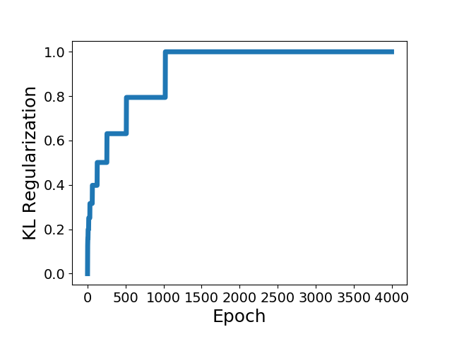
Instead of linearly increasing $\beta$, we suggest a schedule that dedicates more optimization steps to larger $\beta$, making the transition to the full ELBO objective smoother. Specifically, for each $n\in\{0,1,\ldots,N\}$, we train for $2^{n}$ epochs with regularization parameter $\beta_{n}=10^{\frac{n}{N}-1}$ (with $\beta_{0}=0$). We denote with $\mathcal{L}_{n}$ the objective (10) evaluated at $\beta=\beta_{n}$. Observe that the second phase of training ( after $2^{N}$ epochs) is done with the standard VAE objective. The schedule for $\beta_{n}$ for $N=10$ KL levels can be seen in Figure 6(b).

We empirically evaluate the SeRe-VAE on dynamically binarized MNIST. As in [17, 12, 8], the binary-valued observations are sampled after each epoch with the Bernoulli expectations being set equal to the real , normalized pixel values in the dataset which prevents overfitting.

In this section, we validate the variational normalizing flows introduced in Section 4. We used a 5 layer hierarchy of $40$ latent variables each and $T=2$ flows. We adopted a unit rank Gaussian base distribution—parameterized as in Equation (9) in [2]—and diagonal Gaussian prior and posterior layers. We used neural spline generative layers with coupling transformations [23], which boosted the performance compared to the affine transformations. The full architectural and training details are provided in the supplementary material. In Table 3, we compare against generative MAF models with the same or larger width, with or without training dataset augmentation with horizontal image flips and different number of MADEs. Our variational model exhibits significant improvement over the baselines.

We expect further performance improvements could be made by implementing any combination of the following steps: larger MADE layers; more latent features or layers in the hierarchy; a distribution for the decoder that is specific to natural images such as [24, 22]; training with more importance samples [17]; and further finetuning of the architectural or training hyperparameters. However, such optimizations are beyond the scope of this paper and are left for future research.

Table 8 summarizes the hyperparameters of the training process. Below, we describe techniques adopted that are different than those used for the models in the previous experimental studies.

• •

  Due to the complexity of the decoder, which stems from the autoregressive property and the large hidden dimension required in the autoregressive layer, we follow a 3-phase training scheme. First, we minimize only the reconstruction loss (the negative conditional likelihood) of the negative ELBO objective loss, Equation (10), for 350 epochs. Subsequently, we apply geometric warm-up for $N=8$ KL levels (and other 258 epochs). We, finally optimize the rest of the ELBO, for the remaining epochs. For the first phase, we use adaptive learning rate with a cosine scheduler. For the last two phases, a constant learning rate is used.

• •

  The pixel space is converted to logit space by the transformation: $\bm{x}\rightarrow logit(\alpha+(1-\alpha)x)$, for $\alpha=0.05$, after adding uniform noise and rescaling the pixel values in $[0,1]$, as in [16].

• •

  We find applying dropout [51], with probability $0.5$, in the residual blocks of this architecture beneficial for further regularization.

• •

  We employ a free bits strategy, as described in the Appendix C.8, Equation (12), in [8]. In our case, the latent variables are grouped by layer (so that $K$ in Equation (12) in [8] equals $L=4$) with $\lambda_{free_{\_}bits}=1$.

In this section, we describe the construction of the conditional Masked Autoencoders (MADE layers) used as building blocks for the variational normalizing flow presented in Section 5.3. We use notation identical to those used in [34].

Let $C$ be the dimension of the conditioning inputs. $C$ acts as a mask offset in the construction of the masked autoregressive encoder, as we explain below. We assign unique numbers $1,2,\dots,C+D$ to the inputs. In case of a random input ordering, the first $C$ conditioning inputs are excluded so that $m^{0}(d)=d$, for $d=1,2,\dots,C$ and $m^{0}(d)\in\{C+1,C+2,\dots,C+D\}$ uniquely and randomly assigned to the inputs $d=C+1,C+2,\dots,C+D$. The degrees $m^{l}(d)$ of the $d-$th hidden unit of layer $l$ should now be larger than $C$, so that the conditioning inputs are not masked out: the conditioning inputs are connected to all the hidden units. Therefore, $m^{l}(d)$ are random numbers such that $m^{l}(d)\in\{C+1,C+2,C+D\}$. Equation (12) in [34] is still valid for the construction of the masks for connections from the input to the first layer hidden units, and from hidden units to next layer hidden units. For the last layer masks (from the hidden units to the output), Equation (13) in [34] is used, and subsequently the first $C$, that refer to the conditioning inputs, masks are discarded.

Finally, as suggested in [16] batch normalization layers between the MAF steps are incorporated. Section B in the Appendix of [16], provides a description of the batch normalization as a bijector and $tfp.bijectors.BatchNormalization$ [35] offers a suggested implementation. In our implementantion, at both training and validation/test time, we maintain averages over minibatches as in [52].

The trained models can be downloaded from:
https://drive.google.com/file/d/1W_wBTCOM8FouxlJT2IbSYvuwPhpkfpcm/view?usp=sharing

References

- [1] Diederik P. Kingma and Max Welling. Auto-Encoding Variational Bayes. In 2nd International Conference on Learning Representations, ICLR, 2014.
- [2] Danilo Jimenez Rezende, Shakir Mohamed, and Daan Wierstra. Stochastic Backpropagation and Approximate Inference in Deep Generative Models. In Proceedings of the 31st International Conference on Machine Learning , ICML, 2014.
- [3] Florian Wenzel, Kevin Roth, Bastiaan S Veeling, Jakub Świątkowski, Linh Tran, Stephan Mandt, Jasper Snoek, Tim Salimans, Rodolphe Jenatton, and Sebastian Nowozin. How Good is the Bayes Posterior in Deep Neural Networks Really? arXiv preprint arXiv:2002.02405, 2020.
- [4] Andrew Gordon Wilson and Pavel Izmailov. Bayesian Deep Learning and a Probabilistic Perspective of Generalization. arXiv preprint arXiv:2002.08791, 2020.
- [5] Kaiming He, Xiangyu Zhang, Shaoqing Ren, and Jian Sun. Deep Residual Learning for Image Recognition. In The IEEE Conference on Computer Vision and Pattern Recognition, CVPR, June 2016.
- [6] Tim Salimans, Diederik Kingma, and Max Welling. Markov Chain Monte Carlo and Variational Inference: Bridging the Gap. In Proceedings of the 32nd International Conference on Machine Learning, ICML, 2015.
- [7] Ishaan Gulrajani, Kundan Kumar, Faruk Ahmed, Adrien Ali Taïga, Francesco Visin, David Vázquez, and Aaron C. Courville. PixelVAE: A Latent Variable Model for Natural Images. In 5th International Conference on Learning Representations, ICLR, 2017.
- [8] Diederik P Kingma, Tim Salimans, Rafal Jozefowicz, Xi Chen, Ilya Sutskever, and Max Welling. Improved Variational Inference with Inverse Autoregressive Flow. In Advances in Neural Information Processing Systems 29, 2016.
- [9] Xi Chen, Diederik P. Kingma, Tim Salimans, Yan Duan, Prafulla Dhariwal, John Schulman, Ilya Sutskever, and Pieter Abbeel. Variational Lossy Autoencoder. In 5th International Conference on Learning Representations, ICLR, 2017.
- [10] Jakub Tomczak and Max Welling. VAE with a VampPrior. In Proceedings of the Twenty-First International Conference on Artificial Intelligence and Statistics, volume 84 of Proceedings of Machine Learning Research. PMLR, 2018.
- [11] Alexej Klushyn, Nutan Chen, Richard Kurle, Botond Cseke, and Patrick van der Smagt. Learning Hierarchical Priors in VAEs. In Advances in Neural Information Processing Systems 32, 2019.
- [12] Casper Kaae Sø nderby, Tapani Raiko, Lars Maalø e, Søren Kaae Sø nderby, and Ole Winther. Ladder Variational Autoencoders. In Advances in Neural Information Processing Systems 29, 2016.
- [13] Lars Maalø e, Marco Fraccaro, Valentin Liévin, and Ole Winther. BIVA: A Very Deep Hierarchy of Latent Variables for Generative Modeling. In Advances in Neural Information Processing Systems 32, 2019.
- [14] Alexej Klushyn, Nutan Chen, Richard Kurle, Botond Cseke, and Patrick van der Smagt. Learning Hierarchical Priors in VAEs. In Advances in Neural Information Processing Systems 32, 2019.
- [15] Philip Bachman. An architecture for Deep, Hierarchical Generative Models. In Proceedings of the 30th International Conference on Neural Information Processing Systems, 2016.
- [16] George Papamakarios, Theo Pavlakou, and Iain Murray. Masked Autoregressive Flow for Density Estimation. In Advances in Neural Information Processing Systems 30, 2017.
- [17] Yuri Burda, Roger B. Grosse, and Ruslan Salakhutdinov. Importance Weighted Autoencoders. In 4th International Conference on Learning Representations, ICLR, 2016.
- [18] Bin Dai and David P. Wipf. Diagnosing and Enhancing VAE models. In 7th International Conference on Learning Representations, ICLR, 2019.
- [19] Aäron van den Oord, Nal Kalchbrenner, Lasse Espeholt, Koray Kavukcuoglu, Oriol Vinyals, and Alex Graves. Conditional Image Generation with PixelCNN Decoders. In Advances in Neural Information Processing Systems 29, 2016.
- [20] Danilo Jimenez Rezende and Fabio Viola. Taming VAEs. In arXiv preprint arXiv:1810.00597, 2018.
- [21] Laurent Dinh, Jascha Sohl-Dickstein, and Samy Bengio. Density estimation using Real NVP. In 5th International Conference on Learning Representations, ICLR, 2017.
- [22] Diederik P Kingma and Prafulla Dhariwal. Glow: Generative flow with invertible 1x1 convolutions. In Advances in Neural Information Processing Systems 31, 2018.
- [23] Conor Durkan, Artur Bekasov, Iain Murray, and George Papamakarios. Neural spline flows. In Advances in Neural Information Processing Systems 32, 2019.
- [24] Aäron van den Oord, Nal Kalchbrenner, and Koray Kavukcuoglu. Pixel Recurrent Neural Networks. In Proceedings of the 33nd International Conference on Machine Learning, ICML, 2016.
- [25] Karol Gregor, Ivo Danihelka, Alex Graves, Danilo Jimenez Rezende, and Daan Wierstra. DRAW: A Recurrent Neural Network for Image Generation. In Proceedings of the 32nd International Conference on Machine Learning, ICML, 2015.
- [26] Diederik P. Kingma and Max Welling. An Introduction to Variational Autoencoders. Foundations and Trends in Machine Learning, 12(4):307–392, 2019.
- [27] Michael I Jordan. An introduction to probabilistic graphical models, 2003.
- [28] Esteban G. Tabak and Eric Vanden-Eijnden. Density estimation by dual ascent of the log-likelihood. Commun. Math. Sci., 8, 2010.
- [29] E. G. Tabak and Cristina V. Turner. A family of Nonparametric Density Estimation Algorithms. Communications on Pure and Applied Mathematics, 66(2), 2013.
- [30] Walter Rudin. Real and complex analysis. Tata McGraw-hill education, 2006.
- [31] Laurent Dinh, David Krueger, and Yoshua Bengio. NICE: Non-linear independent components estimation. In 3rd International Conference on Learning Representations, ICLR, Workshop Track Proceedings, 2015.
- [32] Danilo Jimenez Rezende and Shakir Mohamed. Variational Inference with Normalizing Flows. In Proceedings of the 32nd International Conference on Machine Learning, ICML, 2015.
- [33] George Papamakarios, Eric Nalisnick, Danilo Jimenez Rezende, Shakir Mohamed, and Balaji Lakshminarayanan. Normalizing Flows for Probabilistic Modeling and Inference. arXiv preprint arXiv:1912.02762, 2019.
- [34] Mathieu Germain, Karol Gregor, Iain Murray, and Hugo Larochelle. MADE: Masked Autoencoder for Distribution Estimation. In Proceedings of the 32nd International Conference on Machine Learning, ICML, 2015.
- [35] TFP Team et al. Tensorflow Probability, 2018–2019. URL https://github. com/tensorflow/probability, 2018.
- [36] Diederik P. Kingma and Jimmy Ba. Adam: A method for stochastic optimization. CoRR, abs/1412.6980, 2015.
- [37] Samuel R. Bowman, Luke Vilnis, Oriol Vinyals, Andrew M. Dai, Rafal Józefowicz, and Samy Bengio. Generating sentences from a Continuous Space. In Proceedings of the 20th SIGNLL Conference on Computational Natural Language Learning, CoNLL. ACL, 2016.
- [38] Casper Kaae Sønderby, Tapani Raiko, Lars Maaløe, Søren Kaae Sønderby, and Ole Winther. How to train deep variational autoencoders and probabilistic ladder networks. In Proceedings of the 33nd International Conference on Machine Learning, ICML, 2016.
- [39] Jason Tyler Rolfe. Discrete Variational Autoencoders. In 5th International Conference on Learning Representations, ICLR, 2017.
- [40] Walter HL Pinaya, Andrea Mechelli, and João R Sato. Using deep autoencoders to identify abnormal brain structural patterns in neuropsychiatric disorders: A large-scale multi-sample study. Human brain mapping, 40, 2019.
- [41] Kuan Han, Haiguang Wen, Junxing Shi, Kun-Han Lu, Yizhen Zhang, Di Fu, and Zhongming Liu. Variational autoencoder: An unsupervised model for encoding and decoding fMRI activity in visual cortex. NeuroImage, 198, 2019.
- [42] Jun Jin Choong, Xin Liu, and Tsuyoshi Murata. Learning community structure with variational autoencoder. In 2018 IEEE International Conference on Data Mining (ICDM). IEEE, 2018.
- [43] Carl Yang, Jieyu Zhang, Haonan Wang, Sha Li, Myungwan Kim, Matt Walker, Yiou Xiao, and Jiawei Han. Relation learning on social networks with multi-modal graph edge variational autoencoders. In Proceedings of the 13th International Conference on Web Search and Data Mining, 2020.
- [44] Nikola Simidjievski, Cristian Bodnar, Ifrah Tariq, Paul Scherer, Helena Andres Terre, Zohreh Shams, Mateja Jamnik, and Pietro Liò. Variational autoencoders for cancer data integration: design principles and computational practice. Frontiers in Genetics, 10, 2019.
- [45] Adam J Riesselman, John B Ingraham, and Debora S Marks. Deep generative models of genetic variation capture the effects of mutations. Nature methods, 15, 2018.
- [46] Samuel I Berchuck, Sayan Mukherjee, and Felipe A Medeiros. Estimating rates of progression and predicting future Visual fields in Glaucoma Using a Deep Variational Autoencoder. Scientific Reports, 9, 2019.
- [47] Chenwei Zhang, Yaliang Li, Nan Du, Wei Fan, and Philip S Yu. On the generative discovery of structured medical knowledge. In Proceedings of the 24th ACM SIGKDD International Conference on Knowledge Discovery & Data Mining, 2018.
- [48] Xiaoyi Deng and Feifei Huangfu. Collaborative variational deep learning for healthcare recommendation. IEEE Access, 7, 2019.
- [49] Lin Yue, Dongyuan Tian, Weitong Chen, Xuming Han, and Minghao Yin. Deep learning for heterogeneous medical data analysis. World Wide Web, 2020.
- [50] Adam Golinski, Reza Pourreza, Yang Yang, Guillaume Sautiere, and Taco S Cohen. Feedback Recurrent Autoencoder for Video Compression. arXiv preprint arXiv:2004.04342, 2020.
- [51] Nitish Srivastava, Geoffrey Hinton, Alex Krizhevsky, Ilya Sutskever, and Ruslan Salakhutdinov. Dropout: a simple way to prevent neural networks from overfitting. The journal of machine learning research, 15(1):1929–1958, 2014.
- [52] Sergey Ioffe and Christian Szegedy. Batch normalization: Accelerating deep network training by reducing internal covariate shift. In Francis Bach and David Blei, editors, Proceedings of the 32nd International Conference on Machine Learning, volume 37 of Proceedings of Machine Learning Research. PMLR, 2015.
7 Experimental Details of the MLP-SeRe VAE for binarized MNIST
This section provides detailed description of the training parameters and architectural hyperparameters for the experiments in Section 5.2.1 in the main paper.
Specifically, in Table 4, we provide the parameters of the training procedure. A constant learning rate and a small amount of weight regularization was used. We did not observe overfitting. Moreover, batch normalization layers were added at the input of each layer in the hierarchy.