Beyond Perturbations: Learning Guarantees with Arbitrary Adversarial Test Examples
Abstract
We present a transductive learning algorithm that takes as input training examples from a distribution and arbitrary (unlabeled) test examples, possibly chosen by an adversary. This is unlike prior work that assumes that test examples are small perturbations of . Our algorithm outputs a selective classifier, which abstains from predicting on some examples. By considering selective transductive learning, we give the first nontrivial guarantees for learning classes of bounded VC dimension with arbitrary train and test distributions—no prior guarantees were known even for simple classes of functions such as intervals on the line. In particular, for any function in a class of bounded VC dimension, we guarantee a low test error rate and a low rejection rate with respect to . Our algorithm is efficient given an Empirical Risk Minimizer (ERM) for . Our guarantees hold even for test examples chosen by an unbounded white-box adversary. We also give guarantees for generalization, agnostic, and unsupervised settings.
1 Introduction
Consider binary classification where test examples are not from the training distribution. Specifically, consider learning a binary function where training examples are assumed to be iid from a distribution over , while the test examples are arbitrary. This includes both the possibility that test examples are chosen by an adversary or that they are drawn from a distribution (sometimes called “covariate shift”). For a disturbing example of covariate shift, consider learning to classify abnormal lung scans. A system trained on scans prior to 2019 may miss abnormalities due to COVID-19 since there were none in the training data. As a troubling adversarial example, consider explicit content detectors which are trained to classify normal vs. explicit images. Adversarial spammers synthesize endless variations of explicit images that evade these detectors for purposes such as advertising and phishing (Yuan et al. 2019).
A recent line of work on adversarial learning has designed algorithms that are robust to imperceptible perturbations. However, perturbations do not cover all types of test examples. In the explicit image detection example, Yuan et al. 2019 find adversaries using conspicuous image distortion techniques (e.g., overlaying a large colored rectangle on an image) rather than imperceptible perturbations. In the lung scan example, Fang et al. 2020 find noticeable signs of COVID in many scans.
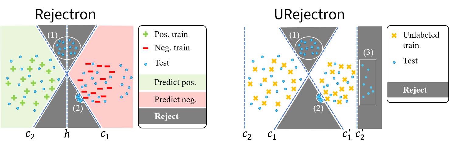
In general, there are several reasons why learning with arbitrary test examples is actually impossible. First of all, one may not be able to predict the labels of test examples that are far from training examples, as illustrated by the examples in group (1) of Figure 1. Secondly, as illustrated by group (2), given any classifier , an adversary or test distribution may concentrate on or near an error. High error rates are thus unavoidable since an adversary can simply repeat any single erroneous example they can find. This could also arise naturally, as in the COVID example, if contains a concentration of new examples near one another–individually they appear “normal” (but are suspicious as a group). This is true even under the standard realizable assumption that the target function is in a known class of bounded VC dimension .
As we now argue, learning with arbitrary test examples requires selective classifiers and transductive learning, which have each been independently studied extensively. We refer to the combination as classification with redaction, a term which refers to the removal/obscuring of certain information when documents are released. A selective classifier (SC) is one which is allowed to abstain from predicting on some examples. In particular, it specifies both a classifier and a subset of examples to classify, and rejects the rest. Equivalently, one can think of a SC as where indicates , abstinence.
We say the learner classifies if and otherwise it rejects . Following standard terminology, if (i.e., ) we say the classifier rejects (the term is not meant to indicate anything negative about the example but merely that its classification may be unreliable). We sat that misclassifies or errs on if . There is a long literature on SCs, starting with the work of Chow 1957 on character recognition. In standard classification, transductive learning refers to the simple learning setting where the goal is to classify a given unlabeled test set that is presented together with the training examples (Vapnik 1998, see e.g.,). We will also consider the generalization error of the learned classifier.
This raises the question: When are unlabeled test examples available in advance? In some applications, test examples are classified all at once (or in batches). Otherwise, redaction can also be beneficial in retrospect. For instance, even if image classifications are necessary immediately, an offensive image detector may be run daily with rejections flagged for inspection; and images may later be blocked if they are deemed offensive. Similarly, if a group of unusual lung scans showing COVID were detected after a period of time, the recognition of the new disease could be valuable even in hindsight. Furthermore, in some applications, one cannot simply label a sample of test examples. For instance, in learning to classify messages on an online platform, test data may contain both public and private data while training data may consist only of public messages. Due to privacy concerns, labeling data from the actual test distribution may be prohibited.
It is clear that a SC is necessary to guarantee few test misclassifications, e.g., if is concentrated on a single point , rejection is necessary to guarantee few errors on arbitrary test points. However, no prior guarantees (even statistical guarantees) were known even for learning elementary classes such as intervals or halfspaces with arbitrary . This is because learning such classes is impossible without unlabeled examples.
To illustrate how redaction (transductive SC) is useful, consider learning an interval on with arbitrary . This is illustrated below with (blue) dots indicating test examples:
![[Uncaptioned image]](2007.05145v3/interval_example.png) |
With positive training examples as in (a), one can guarantee 0 test errors by rejecting the two (grey) regions adjacent to the positive examples. When there are no positive training examples,11 1 Learning with an all-negative training set (trivial in standard learning) is a useful “anomaly detection” setting in adversarial learning, e.g., when one aims to classify illegal images without any illegal examples at train time or abnormal scans not present at train time. as in (b), one can guarantee test errors by rejecting any region with test examples and no training examples; and predicting negative elsewhere. Of course, one can guarantee 0 errors by rejecting everywhere, but that would mean rejecting even future examples distributed like . While our error objective will be an test error rate, our rejection objective will be more subtle since we cannot absolutely bound the test rejection rate. Indeed, as illustrated above, in some cases one should reject many test examples.
Note that our redaction model assumes that the target function remains the same at train and test times. This assumption holds in several (but not all) applications of interest. For instance, in explicit image detection, U.S. laws regarding what constitutes an illegal image are based solely on the image itself (U.S.C. 1996). Of course, if laws change between train and test time, then itself may change. Label shift problems where changes from train to test is also important but not addressed here. Our focus is primarily the well-studied realizable setting, where , though we analyze an agnostic setting as well.
A note of caution.
Inequities may be caused by using training data that differs from the test distribution on which the classifier is used. For instance, in classifying a person’s gender from a facial image, Buolamwini and Gebru 2018 have demonstrated that commercial classifiers are highly inaccurate on dark-skinned faces, likely because they were trained on light-skinned faces. In such cases, it is preferable to collect a more diverse training sample even if it comes at greater expense, or in some cases to abstain from using machine learning altogether. In such cases, learning should not be used, as an unbalanced distribution of rejections can also be harmful.22 2 We are grateful to an anonymous reviewer who pointed out that gender classification is an example of when not to use learning.
1.1 Redaction model and guarantees
Our goal is to learn a target function of VC dimension with training distribution over . In the redaction model, the learner first chooses based on iid training examples and their labels . (In other words, it trains a standard binary classifier.) Next, a “white box” adversary selects arbitrary test examples based on all information including and the learning algorithm. Using the unlabeled test examples (and the labeled training examples), the learner finally outputs . Errors are those test examples in that were misclassified, i.e., .
Rather than jumping straight into the transductive setting, we first describe the simpler generalization setting. We define the model in which are drawn iid by nature, for an arbitrary distribution . While it will be easier to quantify generalization error and rejections in this simpler model, the model does not permit a white-box adversary to choose test examples based on . To measure performance here, define rejection and error rates for distribution , respectively:
| (1) | ||||
| (2) |
We write and when and are clear from context. We extend the definition of PAC learning to as follows:
Definition 1.1 (PQ learning).
Learner -PQ-learns if for any distributions over and any , its output satisfies
PQ-learns if runs in polynomial time and if there is a polynomial such that -PQ-learns for every .
Now, at first it may seem strange that the definition bounds rather than , but as mentioned cannot be bound absolutely. Instead, it can be bound relative to and the total variation distance (also called statistical distance) , as follows:
This new perspective, of bounding the rejection probability of , as opposed to , facilitates the analysis. Of course when , and , and when and have disjoint supports (no overlap), then and the above bound is vacuous. We also discuss tighter bounds relating to .
We provide two redactive learning algorithms: a supervised algorithm called , and an unsupervised algorithm . takes as input labeled training data and test data (and an error parameter ). It can be implemented efficiently using any oracle that outputs a function of minimal error on any given set of labeled examples. It is formally presented in Figure 2. At a high level, it chooses and chooses in an iterative manner. It starts with and then iteratively chooses that disagrees significantly with on but agrees with on ; it then rejects all ’s such that . As we show in Lemma 5.1, choosing can be done efficiently given oracle access to .
Theorem 5.2 shows that PQ-learns any class of bounded VC dimension , specifically with . (The notation hides logarithmic factors including the dependence on the failure probability .) This is worse than the standard bound of supervised learning when , though Theorem 5.4 shows this is necessary with an lower-bound for .
Our unsupervised learning algorithm , formally presented in Figure 3, computes only from unlabeled training and test examples, and has similar guarantees (Theorem 5.6). The algorithm tries to distinguish training and test examples and then rejects whatever is almost surely a test example. More specifically, as above, it chooses in an iterative manner, starting with . It (iteratively) chooses two functions such that and have high disagreement on and low disagreement on , and rejects all ’s on which disagree. As we show in Lemma B.1, choosing and can be done efficiently given a (stronger) oracle for the class of disagreements between . We emphasize that can also be used for multi-class learning as it does not use training labels, and can be paired with any classifier trained separately. This advantage of over comes at the cost of requiring a stronger base classifier to be used for , and may lead to examples being unnecessarily rejected.
In Figure 1 we illustrate our algorithms for the class of halfspaces. A natural idea would be to train a halfspace to distinguish unlabeled training and test examples—intuitively, one can safely reject anything that is clearly distinguishable as test without increasing . However, this on its own is insufficient. See for example group (2) of examples in Figure 1, which cannot be distinguished from training data by a halfspace. This is precisely why having test examples is absolutely necessary. Indeed, it allows us to use an ERM oracle to to PQ-learn .
We also present:
Transductive analysis
A similar analysis of in a transductive setting gives error and rejection bounds directly on the test examples. The bounds here are with respect to a stronger white-box adversary who need not even choose a test set iid from a distribution. Such an adversary chooses the test set with knowledge of and . In particular, first is chosen based on and ; then the adversary chooses the test set based on all available information; and finally, is chosen. We introduce a novel notion of false rejection, where we reject a test example that was in fact chosen from and not modified by an adversary. Theorem 5.3 gives bounds that are similar in spirit to Theorem 5.2 but for the harsher transductive setting.
Agnostic bounds
Thus far, we have considered the realizable setting where the target . In agnostic learning (Kearns et al. 1992), there is an arbitrary distribution over and the goal is to learn a classifier that is nearly as accurate as the best classifier in . In our setting, we assume that there is a known such that the train and test distributions and over satisfy that there is some function that has error at most with respect to both and . Unfortunately, we show that in such a setting one cannot guarantee less than errors and rejections, but we show that nearly achieves such guarantees.
Experiments
As a proof of concept, we perform simple controlled experiments on the task of handwritten letter classification using lower-case English letters from the EMNIST dataset (Cohen et al. 2017). In one setup, to mimic a spamming adversary, after a classifier is trained, test examples are identified on which errs and are repeated many times in the test set. Existing SC algorithms (no matter how robust) will fail on such an example since they all choose without using unlabeled test examples—as long as an adversary can find even a single erroneous example, it can simply repeat it. In the second setup, we consider a natural test distribution which consists of a mix of lower- and upper-case letters, while the training set was only lower-case letters. The simplest version of achieves high accuracy while rejecting mostly adversarial or capital letters.
Organization
2 Related work
The redaction model combines SC and transductive learning, which have each been extensively studied, separately. We first discuss prior work on these topics, which (with the notable exception of online SC) has generally been considered when test examples are from the same distribution as training examples.
Selective classification
Selective classification go by various names including “classification with a reject option” and “reliable learning.” To the best of our knowledge, prior work has not considered SC using unlabeled samples from . Early learning theory work by Rivest and Sloan 1988 required a guarantee of 0 test errors and few rejections. However, Kivinen 1990 showed that, for this definition, even learning rectangles under uniform distributions requires exponential number of examples (as cited by Hopkins et al. 2019 which like much other work therefore makes further assumptions on and ). Most of this work assumes the same training and test distributions, without adversarial modification. Kanade et al. 2009 give a SC reduction to an agnostic learner (similar in spirit to our reduction to ) but again for the case of .
A notable exception is the work in online SC, where an arbitrary sequence of examples is presented one-by-one with immediate error feedback. This work includes the “knows-what-it-knows” algorithm (Li et al. 2011), and Sayedi et al. 2010 exhibit an interesting trade-off between the number of mistakes and the number of rejections in such settings. However, basic classes such as intervals on the line are impossible to learn in these harsh online formulations. Interestingly, our division into labeled train and unlabeled test seems to make the problem easier than in the harsh online model.
Transductive (and semi-supervised) learning.
In transductive learning, the classifier is given test examples to classify all at once or in batches, rather than individually (Vapnik 1998, e.g.,). Performance is measured with respect to the test examples. It is related to semi-supervised learning, where unlabeled examples are given but performance is measured with respect to future examples from the same distribution. Here, since the assumption is that training and test examples are iid, it is generally the case that the unlabeled examples greatly outnumber the training examples, since otherwise they would provide limited additional value.
We now discuss related work which considers , but where classifiers must predict everywhere without the possibility of outputting .
Robustness to Adversarial Examples
There is ongoing effort to devise methods for learning predictors that are robust to adversarial examples (Szegedy et al. 2013; Biggio et al. 2013; Goodfellow et al. 2015) at test time. Such work typically assumes that the adversarial examples are perturbations of honest examples chosen from . The main objective is to learn a classifier that has high robust accuracy, meaning that with high probability, the classifier will answer correctly even if the test point was an adversarially perturbed example. Empirical work has mainly focused on training deep learning based classifiers to be more robust (Madry et al. 2018; Wong and Kolter 2018; Zhang et al. 2019, e.g.,). Kang et al. 2019 consider the fact that perturbations may not be known in advance, and some work (Pang et al. 2018, e.g.,) addresses the problem of identifying adversarial examples. We emphasize that as opposed to this line of work, we consider arbitrary test examples and use SC.
Detecting adversarial examples has been studied in practice, but Carlini and Wagner 2017 study ten proposed heuristics and are able to bypass all of them. Our algorithms also require a sufficiently large set of unlabeled test examples. The use of unlabeled data for improving robustness has also been empirically explored recently (Carmon et al. 2019; Stanforth et al. 2019; Zhai et al. 2019, e.g.,).
In work on real-world adversarial images, Yuan et al. 2019 find adversaries using highly visible transformations rather than imperceptible perturbations. They categorize seven major types of such transformations and write:
“Compared with the adversarial examples studied by the ongoing adversarial learning, such adversarial explicit content does not need to be optimized in a sense that the perturbation introduced to an image remains less perceivable to humans…. today’s cybercriminals likely still rely on a set of predetermined obfuscation techniques… not gradient descent.”
Covariate Shift
The literature on learning with covariate shift is too large to survey here, see, e.g., the book by Quionero-Candela et al. 2009 and the references therein. To achieve guarantees, it is often assumed that the support of is contained in the support of . Like our work, many of these approaches use unlabeled data from (Huang et al. 2007; Ben-David and Urner 2012, e.g.,). Ben-David and Urner 2012 show that learning with covariate-shift is intractable, in the worst case, without such assumptions. In this work we overcome this negative result, and obtain guarantees for arbitrary , using SC. In summary, prior work on covariate shift that guarantees low test/target error requires strong assumptions regarding the distributions. This motivates our model of covariate shift with rejections.
3 Preliminaries and notation
Henceforth, we assume a fixed class of from domain to ,33 3 For simplicity, the theoretical model is defined for binary classification, though our experiments illustrate a multi-class application. To avoid measure-theoretic issues, we assume is countably infinite or finite. and let be the VC dimension of . Let denote the base-2 logarithm and the natural logarithm. The set of functions from to is denoted by . Let the set of subsets of be denoted by . Finally, denotes for any natural number .
4 Learning with redaction
We now describe the two settings for SC. We use the same algorithm in both settings, so it can be viewed as two justifications for the same algorithm. The PQ model provides guarantees with respect to future examples from the test distribution, while the transductive model provides guarantees with respect to arbitrary test examples chosen by an all-powerful adversary. Interestingly, the transductive analysis is somewhat simpler and is used in the PQ analysis.
4.1 PQ learning
In the PQ setting, an SC learner is given labeled examples drawn iid , labels for some unknown , and unlabeled examples . outputs and . The adversary (or nature) chooses based only on and knowledge of the learning algorithm . The definition of PQ learning is given in Definition 1.1. Performance is measured in terms of on future examples from and (rather than the more obvious . Rejection rates on (and ) can be estimated from held out data, if so desired. The quantities can be related and a small implies few rejections on future examples from wherever it “overlaps” with by which we mean for some constant .
Lemma 4.1.
For any and distributions over :
| (3) |
Further, for any
| (4) |
Proof.
For eq. 3, note that one can sample a point from by first sampling and then changing it with probability . This follows from the definition of total variation distance. Thus, the probability that is rejected is at most the probability is rejected plus the probability , establishing eq. 3. To see eq. 4, note
Clearly the above is at most . ∎
If then all that lie in ’s support would necessarily be classified (i.e., ). Note that the bound eq. 3 can be quite loose and a tight bound is given in Appendix G.
It is also worth mentioning that a PQ-learner can also be used to guarantee meaning that it has accuracy with respect to (like a normal PAC learner) but is also simultaneously robust to . The following claim shows this and an additional property that PQ learners can be made robust with respect to any polynomial number of different ’s.
Claim 4.2.
Let and be distributions over . Given a -PQ-learner , , , and additional unlabeled samples , one can generate such that satisfies,
Proof of 4.2.
Let be the blended distribution. Give samples from and each one can straightforwardly construct iid samples . Running gives the guarantee that with prob. , which implies the claim since . ∎
4.2 Transductive setting with white-box adversary
In the transductive setting, there is no and instead empirical analogs and of error and rejection rates are defined as follows, for arbitrary :
| (5) | ||||
| (6) |
Again, and may be omitted when clear from context.
In this setting, the learner first chooses using only and . Then, a true test set is drawn. Based on all available information ( and the code for learner ) the adversary modifies any number of examples from to create arbitrary test set . Finally, the learner chooses based on , and . Performance is measured in terms of rather than , because . One can bound in terms of for any and , as follows:
| (7) |
The hamming distance is the transductive analog of . The following bounds the “false rejections,” those unmodified examples that are rejected:
| (8) |
White-box adversaries
The all-powerful transductive adversary is sometimes called “white box” in the sense that it can choose its examples while looking “inside” rather than using as a black box. While it cannot choose with knowledge of , it can know what will be as a function of if the learner is deterministic, as our algorithms are. Also, we note that the generalization analysis may be extended to a white-box model where the adversary chooses knowing , but it is cumbersome even to denote probabilities over when itself can depend on .
5 Algorithms and guarantees
We assume that we have a deterministic oracle which, given a set of labeled examples from , outputs a classifier of minimal error. Figure 2 describes our algorithm . It takes as input a set of labeled training examples , where and , and a set of test examples along with an error parameter that trades off errors and rejections. A value for that theoretically balances these is in Theorems 5.2 and 5.3.
- •
# assume black box oracle to minimize errors
- •
Lemma 5.1 (Computational efficiency).
For any , , and , outputs for . Further, each iteration can be implemented using one call to on at most examples and evaluations of classifiers in .
Proof.
To maximize using the ERM oracle for , construct a dataset consisting of each training example, labeled by , repeated times, and each test example in , labeled , included just once. Running on this artificial dataset returns a classifier of minimal error on it. But the number of errors of classifier on this artificial dataset is:
which is equal to . Hence minimizes error on this artificial dataset if and only if it maximizes of the algorithm.
Next, let be the number of iterations of the algorithm , so its output is . We must show that . To this end, note that by definition, for every it holds that , and moreover,
| (9) |
Hence, the fraction of additional rejected test examples in each iteration is greater than , and hence . Since is an integer, this means that .
For efficiency, of course each is not explicitly stored since even could be infinite. Instead, note that to execute the algorithm, we only need to maintain: (a) the subset of indices of test examples which are in the prediction set, and (b) the classifiers . Also note that updating from requires evaluating at most times. In this fashion, membership in and can be computed efficiently and output in a succinct manner. ∎
Note that since we assume is deterministic, the algorithm is also deterministic. This efficient reduction to , together with the following imply that is a PQ learner:
Theorem 5.2 (PQ guarantees).
For any and distributions over :
where and .
More generally, Theorem A.5 shows that, by varying parameter , one can achieve any trade-off between and . The analogous transductive guarantee is:
Theorem 5.3 (Transductive).
For any and dist. over :
where and .
One thinks of as the real test examples and as an arbitrary adversarial modification, not necessarily iid. Equation 8 means that this implies errors on unmodified examples. As discussed earlier, the guarantee above holds for any chosen by a white-box adversary, which may depend on and , and thus on (since is determined by and ). More generally, Theorem A.2 shows that, by varying parameter , one can trade-off and
We note that Theorems 5.2 and 5.3 generalize in a rather straightforward manner to the case in which an adversary can inject additional training examples to form which contains . Such an augmentation reduces the version space, i.e., the set of consistent with on , but of course still remains in this set. The analysis remains essentially unchanged as long as contains and consists of examples. The bounds remain the same in terms of , but should be run with larger than the number of examples in in this case to ensure that each has zero training error.
Here we give the proof sketch of Theorem 5.3, since it is slightly simpler than Theorem 5.2. Full proofs are in Appendix A.
Proof sketch for Theorem 5.3.
To show , fix any . Since and , this implies that has zero training error, i.e., . Hence and the algorithm cannot terminate with since it could have selected .
To prove , observe that never rejects any training . This follows from the fact that , together with the fact that for every which follows, in turn, from the facts that and . Now and are identically distributed. By a generalization-like bound (Lemma A.1), with probability there is no classifier for which selects all of and yet rejects with probability greater than on for (by Lemma 5.1). ∎
Unfortunately, the above bounds are worse than standard VC-bounds for , but the following lower-bound shows that is tight for some class .
Theorem 5.4 (PQ lower bound).
There exists a constant such that: for any , there is a concept class of VC dimension , distributions and , such that for any and learner , there exists with
Note that since and are fixed, independent of the learner , the unlabeled test examples from are not useful for the learner as they could simulate as many samples from as they would like on their own. Thus, the lower bound holds even given training examples and unlabeled test examples, for arbitrarily large .
Theorem 5.4 implies that the learner needs at least labeled training examples to get the error plus rejection guarantee. However, it leaves open the possibility that many fewer than test examples are needed. We give a lower bound in the transductive case which shows that both must be at least :
Theorem 5.5 (Transductive lower bound).
There exists a constant such that: for any there exists a concept class of VC dimension where, for any there exists a distribution , and an adversary , such that for any learner there is a function such that:
where and .
This lower bound implies that one needs both training and test examples to guarantee error plus rejections. This is partly why, for simplicity, aside from the Theorem 5.5, our analysis takes . The proofs of these two lower bounds are in Appendix F.
- •
Unsupervised selection algorithm.
Our unsupervised selection algorithm is described in Figure 3. It takes as input only train and test examples along with an error parameter recommended to be , and it outputs a set of the selected elements. requires a more powerful black-box ERM—we show that can be implemented efficiently if one can perform ERM with respect to the family of binary classifiers that are disagreements (xors) between two classifiers. For classifiers , define and as follows:
| (10) |
Lemma B.1 shows how is implemented efficiently with an oracle.
Also, we show nearly identical guarantees to those of Theorem 5.3 for :
Theorem 5.6 (Unsupervised).
For any , any , and any distribution over :
where , and
The proof is given in Appendix B and follows from Theorem B.2 which shows that by varying parameter , one can achieve any trade-off and . Since one runs without labels, it has guarantees with respect to any empirical risk minimizer which may be chosen separately, and its output is also suitable for a multi-class problem.
Massart noise.
We also consider two non-realizable models. First, we consider the Massart noise model, where there is an arbitrary (possibly adversarial) noise rate chosen for each example. We show that is a PQ learner in the Massart noise model with , assuming an ERM oracle and an additional examples from . See Appendix C for details.
A semi-agnostic setting.
We also consider the following semi-agnostic model. For an arbitrary distribution over , again with , the analogous notions of rejection and error are:
In standard agnostic learning with respect to , we suppose there is some classifier with error and we aim to find a classifier whose generalization error is not much greater than . In that setting, one can of course choose . For well-fitting models, where there is some classifier with very low error, may be small.
To prove any guarantees in our setting, the test distribution must somehow be related to the training distribution. To tie together the respective training and test distributions over , we suppose we know such that both and for some . Even with these conditions, Lemma D.1 shows that one cannot simultaneously guarantee error rate on and rejection rate on less than , and Theorem D.2 shows that our algorithm achieves a similar upper bound. This suggests that PQ-learning (i.e., adversarial SC) may be especially challenging in settings where ML is not able to achieve low error .
6 Experiments
Rather than classifying sensitive attributes such as explicit images, we perform simple experiments on handwritten letter classification from the popular EMNIST dataset (Cohen et al. 2017). For both experiments, the training data consisted of the eight lowercase letters a d e h l n r t, chosen because they each had more than 10,000 instances. From each letter, 3,000 instances of each letter were reserved for use later, leaving 7,000 examples, each constituting 56,000 samples from .
We then considered two test distributions, representing adversarial and natural settings. consisted of a mix of 50% samples from (the 3,000 reserved instances per lower-case letter mentioned above) and 50% samples from an adversary that used a classifier as a black box. To that, we added 3,000 adversarial examples for each letter selected as follows: the reserved 3,000 letters were labeled by and the adversary selected the first misclassified instance for each letter. Misclassified examples are shown in Figure 5. It made 3,000 imperceptible modifications of each of the above instances by changing the intensity value of a single pixel by at most 4 (out of 256). The result was 6,000 samples per letter constituting 48,000 samples from .


For , the test set also consisted of 6,000 samples per letter, with 3,000 reserved samples from as above. In this case, the remaining half of the letters were simply upper-case44 4 In some datasets, letter classes consist of a mix of upper- and lower-case, while in others they are assigned different classes (EMNIST has both types of classes). In our experiments, they belong to the same class. versions of the letters A D E H L N R T, taken from the EMNIST dataset (case information is also available in that dataset). Again the dataset size is 48,000. We denote this test distribution by .
In Figure 4, we plot the trade-off between the rejection rate on and the error rate on of the algorithm. Since this is a multi-class problem, we implement the most basic form of the algorithm, with iterations. Instead of fixing parameter , we simply train a predictor to distinguish between examples from and , and train a classifier on . We trained two models, a random forest (with default parameters from scikit-learn (Pedregosa et al. 2011)) and a neural network. Complete details are provided at the end of this section. We threshold the prediction scores of distinguisher at various values. For each threshold , we compute the fraction of examples from that are rejected (those with prediction score less than ), and similarly for , and the error rate of classifier on examples from that are not rejected (those with prediction score at least ). We see in Figure 4 that for a suitable threshold our algorithm achieves both low rejection rate on and low error rate on . Thus on these problems the simple algorithm suffices.
We compare to the state-of-the-art SC algorithm SelectiveNet (Geifman and El-Yaniv 2019). We ran it to train a selective neural network classifier on . SelectiveNet performs exceptionally on , achieving low error and reject almost exclusively upper-case letters. It of course errs on all adversarial examples from , as will all existing SC algorithms (no matter how robust) since they all choose without using unlabeled test examples.
Models
A Random Forest Classifier from Scikit-Learn (default parameters including 100 estimators) (Pedregosa et al. 2011) and a simple neural network consisting of two convolutional layers followed by two fully connected layers55 5 https://github.com/pytorch/examples/blob/master/mnist/main.py were fit on a stratified 90%/10% train/test split. The network parameters are trained with SGD with momentum (), weight decay (), batch size (), for epochs with a learning rate of , that is decayed it by a factor of 10 on epochs 57 and 72. had a 3.6% test error rate on , and had a 1.3% test error rate on .
SelectiveNet
SelectiveNet requires a target coverage hyperparameter which in our experiments is fixed to 0.7. We use an open-source PyTorch implementation of SelectiveNet that is available on GitHub 66 6 https://github.com/pranaymodukuru/pytorch-SelectiveNet, with a VGG 16 architecure (Simonyan and Zisserman 2015). To accommodate the VGG 16 architecure without changes, we pad all images with zeros (from 28x28 to 32x32), and duplicate the channels (from 1 to 3). SelectiveNet achieves rejection rates of 21.08% (), 45.89% (), and 24.04% (), and error rates of 0.02% (), 0.81% (), and 76.78% ().

7 Conclusions
The fundamental theorem of statistical learning states that an algorithm for class is asymptotically nearly optimal requiring labeled examples for learning arbitrary distributions when (Shalev-Shwartz and Ben-David 2014, see, e.g.,). This paper can be viewed as a generalization of this theorem to the case where , obtaining rates. When , unlabeled samples from are readily available by ignoring labels of some training data, but unlabeled test samples are necessary when . No prior such guarantee was known for arbitrary , even for simple classes such as intervals, perhaps because it may have seemed impossible to guarantee anything meaningful in the general case.
The practical implications are that, to address learning in the face of adversaries beyond perturbations (or drastic covariate shift), unlabeled examples and abstaining from classifying may be necessary. In this model, the learner can beat an unbounded white-box adversary. Even the simple approach of training a classifier to distinguish unlabeled train vs. test examples may be adequate in some applications, though for theoretical guarantees one requires somewhat more sophisticated algorithms.
Broader Impact
In adversarial learning, this work can benefit users when adversarial examples are correctly identified. It can harm users by misidentifying such examples, and the misidentifications of examples as suspicious could have negative consequences just like misclassifications. This work ideally could benefit groups who are underrepresented in training data, by abstaining rather than performing harmful incorrect classification. However, it could also harm such groups: (a) by providing system designers an alternative to collecting fully representative data if possible; (b) by harmfully abstaining at different rates for different groups; (c) when those labels would have otherwise been correct but are instead being withheld; and (d) by identifying them when they would prefer to remain anonymous.
Our experiments on handwriting recognition have few ethical concerns but also have less ecological validity than real-world experiments on classifying explicit images or medical scans.
References
- Bardenet et al. [2015] Rémi Bardenet, Odalric-Ambrym Maillard, et al. Concentration inequalities for sampling without replacement. Bernoulli, 21(3):1361–1385, 2015.
- Ben-David and Urner [2012] Shai Ben-David and Ruth Urner. On the hardness of domain adaptation and the utility of unlabeled target samples. In Nader H. Bshouty, Gilles Stoltz, Nicolas Vayatis, and Thomas Zeugmann, editors, Algorithmic Learning Theory, pages 139–153, Berlin, Heidelberg, 2012. Springer Berlin Heidelberg. ISBN 978-3-642-34106-9.
- Biggio et al. [2013] Battista Biggio, Igino Corona, Davide Maiorca, Blaine Nelson, Nedim Šrndić, Pavel Laskov, Giorgio Giacinto, and Fabio Roli. Evasion attacks against machine learning at test time. In Joint European conference on machine learning and knowledge discovery in databases, pages 387–402. Springer, 2013.
- Blumer et al. [1989] Anselm Blumer, A. Ehrenfeucht, David Haussler, and Manfred K. Warmuth. Learnability and the vapnik-chervonenkis dimension. J. ACM, 36(4):929–965, October 1989. ISSN 0004-5411. doi: 10.1145/76359.76371. URL https://doi.org/10.1145/76359.76371.
- Buolamwini and Gebru [2018] Joy Buolamwini and Timnit Gebru. Gender shades: Intersectional accuracy disparities in commercial gender classification. In Conference on fairness, accountability and transparency, pages 77–91, 2018.
- Carlini and Wagner [2017] Nicholas Carlini and David Wagner. Adversarial examples are not easily detected: Bypassing ten detection methods. In Proceedings of the 10th ACM Workshop on Artificial Intelligence and Security, pages 3–14. ACM, 2017.
- Carmon et al. [2019] Yair Carmon, Aditi Raghunathan, Ludwig Schmidt, John C Duchi, and Percy S Liang. Unlabeled data improves adversarial robustness. In Advances in Neural Information Processing Systems, pages 11190–11201, 2019.
- Chow [1957] Chi-Keung Chow. An optimum character recognition system using decision functions. IRE Transactions on Electronic Computers, (4):247–254, 1957.
- Cohen et al. [2017] Gregory Cohen, Saeed Afshar, Jonathan Tapson, and Andre Van Schaik. Emnist: Extending mnist to handwritten letters. In 2017 International Joint Conference on Neural Networks (IJCNN), pages 2921–2926. IEEE, 2017.
- Fang et al. [2020] Yicheng Fang, Huangqi Zhang, Jicheng Xie, Minjie Lin, Lingjun Ying, Peipei Pang, and Wenbin Ji. Sensitivity of chest ct for covid-19: comparison to rt-pcr. Radiology, page 200432, 2020.
- Geifman and El-Yaniv [2019] Yonatan Geifman and Ran El-Yaniv. Selectivenet: A deep neural network with an integrated reject option. In Kamalika Chaudhuri and Ruslan Salakhutdinov, editors, Proceedings of the 36th International Conference on Machine Learning, ICML 2019, 9-15 June 2019, Long Beach, California, USA, volume 97 of Proceedings of Machine Learning Research, pages 2151–2159. PMLR, 2019. URL http://proceedings.mlr.press/v97/geifman19a.html.
- Goodfellow et al. [2015] Ian J. Goodfellow, Jonathon Shlens, and Christian Szegedy. Explaining and harnessing adversarial examples. In Proceedings of the 3rd International Conference on Learning Representations, ICLR, 2015. URL http://arxiv.org/abs/1412.6572.
- Hopkins et al. [2019] Max Hopkins, Daniel M Kane, and Shachar Lovett. The power of comparisons for actively learning linear classifiers. arXiv preprint arXiv:1907.03816, 2019.
- Huang et al. [2007] Jiayuan Huang, Arthur Gretton, Karsten Borgwardt, Bernhard Schölkopf, and Alex J Smola. Correcting sample selection bias by unlabeled data. In Advances in neural information processing systems, pages 601–608, 2007.
- Kanade et al. [2009] Varun Kanade, Adam Tauman Kalai, and Yishay Mansour. Reliable agnostic learning. In Proceedings of the 22nd Annual Conference on Learning Theory (COLT), 2009, June 2009. URL https://www.microsoft.com/en-us/research/publication/reliable-agnostic-learning/.
- Kang et al. [2019] Daniel Kang, Yi Sun, Dan Hendrycks, Tom Brown, and Jacob Steinhardt. Testing robustness against unforeseen adversaries. arXiv preprint arXiv:1908.08016, 2019.
- Kearns et al. [1992] Michael J. Kearns, Robert E. Schapire, Linda M. Sellie, and Lisa Hellerstein. Toward efficient agnostic learning. In In Proceedings of the Fifth Annual ACM Workshop on Computational Learning Theory, pages 341–352, 1992.
- Kivinen [1990] Jyrki Kivinen. Reliable and useful learning with uniform probability distributions. In Proceedings of the First International Workshop on Algorithmic Learning Theory (ALT), pages 209–222, 1990.
- Li et al. [2011] Lihong Li, Michael L Littman, Thomas J Walsh, and Alexander L Strehl. Knows what it knows: a framework for self-aware learning. Machine learning, 82(3):399–443, 2011.
- Madry et al. [2018] Aleksander Madry, Aleksandar Makelov, Ludwig Schmidt, Dimitris Tsipras, and Adrian Vladu. Towards deep learning models resistant to adversarial attacks. In 6th International Conference on Learning Representations, ICLR 2018, Vancouver, BC, Canada, April 30 - May 3, 2018, Conference Track Proceedings, 2018. URL https://openreview.net/forum?id=rJzIBfZAb.
- Massart et al. [2006] Pascal Massart, Élodie Nédélec, et al. Risk bounds for statistical learning. The Annals of Statistics, 34(5):2326–2366, 2006.
- Pang et al. [2018] Tianyu Pang, Chao Du, Yinpeng Dong, and Jun Zhu. Towards robust detection of adversarial examples. In Advances in Neural Information Processing Systems, pages 4579–4589, 2018.
- Pedregosa et al. [2011] Fabian Pedregosa, Gaël Varoquaux, Alexandre Gramfort, Vincent Michel, Bertrand Thirion, Olivier Grisel, Mathieu Blondel, Peter Prettenhofer, Ron Weiss, Vincent Dubourg, et al. Scikit-learn: Machine learning in python. the Journal of machine Learning research, 12:2825–2830, 2011.
- Quionero-Candela et al. [2009] Joaquin Quionero-Candela, Masashi Sugiyama, Anton Schwaighofer, and Neil D Lawrence. Dataset shift in machine learning. 2009.
- Rivest and Sloan [1988] Ronald L. Rivest and Robert [H.] Sloan. Learning complicated concepts reliably and usefully (extended abstract). In Tom Mitchell and Reid Smith, editors, Proceedings AAAI-88, pages 635–640. AAAI, 1988.
- Sayedi et al. [2010] Amin Sayedi, Morteza Zadimoghaddam, and Avrim Blum. Trading off mistakes and don’t-know predictions. In Advances in Neural Information Processing Systems, pages 2092–2100, 2010.
- Shalev-Shwartz and Ben-David [2014] Shai Shalev-Shwartz and Shai Ben-David. Understanding Machine Learning: From Theory to Algorithms. Cambridge university press, 2014.
- Simonyan and Zisserman [2015] Karen Simonyan and Andrew Zisserman. Very deep convolutional networks for large-scale image recognition. In Yoshua Bengio and Yann LeCun, editors, 3rd International Conference on Learning Representations, ICLR 2015, San Diego, CA, USA, May 7-9, 2015, Conference Track Proceedings, 2015. URL http://arxiv.org/abs/1409.1556.
- Stanforth et al. [2019] Robert Stanforth, Alhussein Fawzi, Pushmeet Kohli, et al. Are labels required for improving adversarial robustness? arXiv preprint arXiv:1905.13725, 2019.
- Szegedy et al. [2013] Christian Szegedy, Wojciech Zaremba, Ilya Sutskever, Joan Bruna, Dumitru Erhan, Ian Goodfellow, and Rob Fergus. Intriguing properties of neural networks. arXiv preprint arXiv:1312.6199, 2013.
- U.S.C. [1996] U.S.C. 18 u.s.c. §§ 2252, 2252a., child pornography prevention act, 1996.
- Vapnik [1998] Vladimir N. Vapnik. Statistical Learning Theory. Wiley-Interscience, 1998.
- Wong and Kolter [2018] Eric Wong and Zico Kolter. Provable defenses against adversarial examples via the convex outer adversarial polytope. In International Conference on Machine Learning, pages 5283–5292, 2018.
- Yuan et al. [2019] Kan Yuan, Di Tang, Xiaojing Liao, Xiaofeng Wang, Xuan Feng, Yi Chen, Menghan Sun, Haoran Lu, and Kehuan Zhang. Stealthy porn: Understanding real-world adversarial images for illicit online promotion. 2019 IEEE Symposium on Security and Privacy (SP), pages 952–966, 2019.
- Zhai et al. [2019] Runtian Zhai, Tianle Cai, Di He, Chen Dan, Kun He, John Hopcroft, and Liwei Wang. Adversarially robust generalization just requires more unlabeled data. arXiv preprint arXiv:1906.00555, 2019.
- Zhang et al. [2019] Hongyang Zhang, Yaodong Yu, Jiantao Jiao, Eric Xing, Laurent El Ghaoui, and Michael Jordan. Theoretically principled trade-off between robustness and accuracy. In International Conference on Machine Learning, pages 7472–7482, 2019.
Appendix A Rejectron analysis (realizable)
In this section, we present the analysis of in the realizable case . Say a classifier is consistent if makes 0 training errors. Theorem 5.3 provides transductive guarantees on the empirical error and rejection rates, while Theorem 5.2 provides generalization guarantees that apply to future examples from . Both of these theorems exhibit trade-offs between error and rejection rates. At a high level, their analysis has the following structure:
- •
selects a consistent , since we are in the realizable case.
- •
Each is a consistent classifier that disagrees with on the tests as much as possible, with (since ). This follows the facts that , , and for any inconsistent . (The algorithm is defined for general for the agnostic analysis later.)
- •
Therefore, when the algorithm terminates on iteration , it has empirical test error otherwise it could have chosen .
- •
The number of iterations since on each iteration an additional fraction of is removed from . Lemma 5.1 states this and shows how to use an oracle on an artificial dataset to efficiently find .
- •
All training examples are in since each and agree on all .
- •
Transductive error and rejection bounds:
- 1.
For error, we have already argued that the empirical error .
- 2.
For rejection, Lemma A.1 states that it is unlikely that there would be any choice of where the resulting would contain all training examples but reject (abstain on) many “true” test examples since and are identically distributed. The proof uses Sauer’s lemma.
- 1.
- •
We next move to the transductive analysis since it is simpler, and it is also used as a stepping stone to the generalization analysis.
A.1 Transductive guarantees (realizable)
Note that rejects any , where is defined by
| (11) |
In what follows, we prove the transductive analogue of a “generalization” guarantee for arbitrary . This will be useful when proving Theorem 5.3.
Lemma A.1.
For any , any , and :
This lemma is proven in Appendix E. Using it, we can show a trade-off between error and rejection rate for the transductive case.
Theorem A.2.
For any , any , any :
| (12) |
where , and for any distribution over ,
| (13) |
We note that a natural alternative formalization of Equation (13) would be to require that
However, the formalization of Equation (13) is stronger, as it guarantees that the rejection probability is small, even if the adversary is “white-box" and chooses after seeing .
Proof of Theorem A.2.
We start by proving eq. 12. To this end, fix any , any , any , and any . Let . Since we are in the realizable case, this implies that has zero training error, i.e., , and hence for all . Thus, the algorithm cannot terminate on any iteration where since it can always select . This proves Equation (12).
It remains to prove eq. 13. By Lemma 5.1, is an upper bound on the number of completed iterations of the algorithm. WLOG there are exactly iterations because if there were actually iterations, simply “pad” them with which doesn’t change .
We note that the algorithm selects all training examples. This follows from the fact that , together with the fact that for every , where the latter follows from the fact that and . By Lemma A.1, with probability there are no choices for which contains all ’s but is missing fraction of for since . ∎
Theorem 5.3 is a trivial corollary of Theorem A.2.
Proof of Theorem 5.3.
A.2 Generalization guarantees (realizable)
Before we state our generalization guarantees, analogous to Lemma A.1 above, we prove that low test error and low training rejection rates imply, with high probability, low generalization error and rejection rates.
Lemma A.3.
For any , , any and any distribution over ,
Lemma A.4.
For any , any and any distribution over ,
where . Also,
for any .
We mention that the first inequality in Lemma A.4 is used to provide generalization guarantees in the realizable setting, whereas the latter inequality is used to provide guarantees in the semi-agnostic setting.
Theorem A.5.
For any and , any , any and any distributions over :
| (14) |
where . Furthermore, for any ,
| (15) |
Proof of Theorem A.5.
Let be an upper bound on the number of iterations. We first prove eq. 14. Since the ERM algorithm is assumed to be deterministic, the function is uniquely determined by and . By Theorem A.2 (Equation (12)), the set has the property that (with certainty) for all . By Lemma A.3, with probability at most there exists a choice of which would lead to and , implying eq. 14.
Theorem 5.2 is a trivial corollary of Theorem A.5.
Proof of Theorem 5.2.
Recall that .
Equation 14 implies that and eq. 15 implies,
Further, note that for and hence, using ,
The proof is completed by the union bound. ∎
Appendix B Analysis of Urejectron
In this section we present a transductive analysis of , again in the realizable case. We begin with its computational efficiency.
Lemma B.1 ( computational efficiency).
For any and , outputs for . Further, each iteration can be implemented using one call to , as defined in eq. 10, on at most examples and evaluations of classifiers in .
The proof of this lemma is nearly identical to that of Lemma 5.1.
Proof of Lemma B.1.
The argument that follows for the same reason as before, replacing eq. 9 with:
For efficiency, again all that needs to be stored are the subset of indices and the classifiers necessary to compute . To implement iteration using the oracle, construct a dataset consisting of each training example, labeled by 0, repeated times, and each test example in , labeled , included just once. The accuracy of on this dataset is easily seen to differ by a constant from , hence running maximizes . ∎
The following Theorem exhibits the trade-off between accuracy and rejections.
Theorem B.2.
For any , any ,
| (16) |
where and . Furthermore, for any and any distribution over :
| (17) |
Before we prove Theorem B.2 we provide some generalization bounds that will be used in the proof. To this end, given a family of classifiers , following Blumer et al. 1989, define:
| (18) |
Lemma B.3 (Transductive train-test bounds).
For any , any distribution over a domain , any set of classifiers over , and any ,
| (19) |
and
| (20) |
The proof of this lemma is deferred to Appendix E. (Note eq. 20 is used for the agnostic analysis later.)
Proof of Theorem B.2.
We denote for and classifier vectors :
Thus the output of is for the vectors and chosen by the algorithm.
Let be the final iteration of the algorithm so that the output of the algorithm is . Note that , by definition of , so (otherwise the algorithm would have chosen instead of halting) which implies eq. 16.
By Lemma B.1, WLOG we can take by padding with classifiers .
We next claim that for all , i.e., . This is because the algorithm is run with , so any disagreement would result in a negative score . (But a zero score is always possible by choosing .) Thus we must have the property that and hence . Now, it is not difficult to see that because, by Sauer’s lemma, there are at most different labelings of examples by classifiers from , hence there are at most disagreement labelings for pairs. Thus for , by Lemma B.3,
If this likely event happens, then also for the algorithm choices . ∎
Proof of Theorem 5.6.
Appendix C Massart Noise
This section shows that we can PQ learn in the Massart noise model. The Massart model [Massart et al. 2006] is defined with respect to a noise rate and function (abusing notation) :
Definition C.1 (Massart Noise Model).
Let be a distribution on , , and for all . The Massart distribution with respect to over is defined as follows: first is chosen and then with probability and with probability .
When clear from context, we omit and write . The following lemma relates the clean error rate and noisy error rate . Later, we will show how to drive the clean error arbitrarily close to 0 using an ERM.
Lemma C.2.
For any classifier , any , and any distribution corrupted with Massart noise:
where .
Proof.
By definition of the noisy error rate of under , observe the following:
where the last inequality follows from the fact that for every . Rearranging the terms concludes the proof. ∎
The following lemma shows that using an extra i.i.d. examples , we can “denoise” the held-out examples with , and then run on . This shows that we can PQ learn under Massart noise.
Lemma C.3 (Massart denoising).
For any and any distribution over , any and , let be the corresponding Massart distribution over . For any , let be i.i.d. examples sampled from . Then,
where and .
Proof.
By agnostic learning guarantees for , we have that for any :
where and . By Lemma C.2, choosing guarantees that the clean error rate . Since, are independent held-out examples, by a union bound, we get that with probability . ∎
This yields an easy algorithm and corollary: simply use the examples to denoise the labels for and then run the algorithm.
Corollary C.4 (PQ guarantees under Massart noise).
For any and distributions over , any and , let be the corresponding Massart distribution over . Then,
where , , , and .
Appendix D Semi-agnostic analysis
In agnostic learning, the learner is given pairs from some unknown distribution , and it is assumed that there exists some (unknown) such that
In this work, we consider the case where the test distribution may be (arbitrarily) different from the train distribution , yet we require the existence of parameters and an (unknown) such that
Moreover, in this work we assume that and are known. Unfortunately, even with this additional assumption, agnostic learning is challenging when and one cannot achieve guarantees near as one would hope, as we demonstrate below.
In what follows, we slightly abuse notation and write to denote drawn iid from for . The definitions of error and rejection with respect to such a distribution are:
We prove the following lower bound.
Lemma D.1.
There exists a family of binary classifiers of VC dimension 1, such that for any and , and for any selective classification algorithm there exists over and such that:
where and where and .
The proof is deferred to Section F.
We now show that can be used to achieve nearly this guarantee. Recall that in the realizable setting, we fixed in . In this semi-agnostic setting, we will set as a function of , hence our learner requires knowledge of unlike standard agnostic learning when .
Theorem D.2 (Agnostic generalization).
For any , any , any , and any distributions over such that that and simultaneously for some :
where , , and .
A few points of comparison are worth making:
- •
When , one recovers guarantees that are slightly worse than those in the realizable (see Theorem 5.2).
- •
In standard agnostic learning, where and are identical, and thus , one can set (i.e., select everything) and ERM guarantees w.h.p. for sufficiently large.
- •
The above theorem can be used to bound using the following lemma:
Lemma D.3.
For any , and distributions over :
where are the marginal distributions of over .
Proof.
The lemma follows from Lemma 4.1 applied to , and from the fact that the total variation between marginal distributions is no greater than the originals: .∎
As before, it will be useful (and easier) to first analyze the transductive case. In this case, it will be useful to further abuse notation and define, for any ,
Using this, we will show:
Theorem D.4 (Agnostic transductive).
For any , , :
| (21) |
where . Furthermore,
| (22) |
The above bounds suggest the natural choice of if . The following two Lemmas will be used in its proof.
Lemma D.5.
For any , , : where .
Proof.
Note that for each iteration of the algorithm ,
because maximizes the above quantity over , and that quantity is zero at . Also note that if and only if for some . More specifically, for each such that there exists a unique such that , and yet , where the latter occurs when . Thus the total number of test and train rejections can be related as follows:
Dividing both sides by gives the lemma. ∎
The following lemma is proven in Appendix E.
Lemma D.6.
For any , any , and :
Using these, we can now prove the transductive agnostic theorem.
Proof of Theorem D.4.
To prove Equation (21), first fix any . Since the output satisfies . By the triangle inequality, this implies that
| (23) |
Now suppose the algorithm terminates on iteration and the output is for . Then by definition, for every ,
For in particular,
Equation 21 follows from the above and the fact that
Returning to the generalization (distributional) agnostic case, the following theorem shows the trade-off between error and rejections:
Theorem D.7.
For any and , any , any , and any distributions over :
| (24) |
where . Furthermore,
| (25) |
The proof of this theorem will use the following lemma.
Lemma D.8.
For any , distribution over , and
The proof of this lemma is deferred to Appendix E.
Proof of Theorem D.7.
The proof structure follows the proof of Theorem A.5. Fix . We start by proving Equation (24). Let By Lemma D.8,
Since , multiplicative Chernoff bounds imply that,
Also, since , additive Chernoff bounds imply that,
Combining previous four displayed inequalities, which by the union bound all hold with probability , gives,
Simplifying:
| (26) |
Next, we note that for our requirement of , because:
Thus we can remove the maximum from eq. 26,
which is equivalent to what needed to prove in eq. 24.
We next prove eq. 25. By Lemma D.5, with certainty. So by Lemma E.2 (Equation 34) with ,
for using . This implies eq. 25 using the fact that,
∎
From this theorem, our main agnostic upper-bound follows in a straightforward fashion.
Proof of Theorem D.2.
Note that for our choice of ,
using the fact that . For the chosen , Theorem D.7 implies,
| (27) |
Also note that
Theorem D.7 also implies:
| (28) |
where we have used Lemma D.3 in the last step. The union bound over eq. 27 and eq. 28 proves the corollary. ∎
Appendix E Generalization Lemmas
In this section we state auxiliary lemmas that relate the empirical error and rejection rates to generalization error and rejection rates.
To bound generalization, it will be useful to note that the classifiers output by our algorithm are not too complex. To do this, for any and any classifiers , define the disagreement function that is 1 if any of two disagree on :
| (29) |
Also denote by and . In these terms we can write,
Recall the definition of for a family of classifiers :
Lemma E.1 (Complexity of output class).
For any , let
| (30) |
| (31) |
| (32) |
Then , , and , where is the VC dimension of .
Proof.
The proof follows trivially from Sauer’s lemma, since the number of labelings of examples by any is at most and there are choices of and 1 choice of . ∎
Lemma E.2 (Generalization bounds using Blumer et al. 1989).
For any , any distribution over a domain , any set of binary classifiers over , and any ,
| (33) |
and, for any
| (34) |
Finally, for any distribution over and any
| (35) |
Proof.
Simply consider a binary classification problem where the target classifier is the constant 0 function, with training examples . Then the training error rate is and the generalization error is . By Theorem A2.1 of Blumer et al. 1989, the probability that any has 0 training error and test error greater than is at most . Similarly eq. 34 and (35) follow from Theorem A3.1 of Blumer et al. 1989, noting that the bound holds trivially for all with . ∎
We now prove Lemma D.8, which adapts the last bound above to the agnostic setting.
Proof of Lemma D.8.
We would like to apply the last inequality of Lemma E.2 with , but unfortunately that lemma does not apply to error rates of selective classifiers. First, consider the case where the distribution is “consistent” in that for some arbitrary . We can consider the modified functions,
It follows that . Furthermore, the class satisfies (just as we argued ) because there are different labelings of on elements and thus there are at most choices of of these for . Thus, applying Lemma E.2 gives the lemma for consistent .
The inconsistent case can be reduced to the consistent case by a standard trick. In particular, we will extend to by appending a latent (hidden) copy of , call it , to each example . In particular For , define so that the classifiers cannot depend on . This does not change the VC dimension of the classifiers. However, now, any distribution over can be converted to a consistent distribution over whose marginal distribution over agrees with , by making
In other words, . Now, clearly is consistent. The statement of the lemma applied to implies the corresponding statement for since the classifiers do not depend on . ∎
We now prove Lemma B.3.
Proof of Lemma B.3.
Fix any , any distribution over a domain and any . Imagine selecting by first randomly choosing random elements and then randomly dividing these elements into two equal sized sequences . Let denote the distribution over the such divisions . For any and , we claim:
To see this, suppose (otherwise the probability above is zero). The probability that all of them are in the test set is at most because the chance that the first rejection is placed in the test set is , the second is , and so forth. The above equation directly implies eq. 19 by dividing by .
We now move to eq. 20. Consider random variables and . It suffices to show that that with probability for . Note that since ,
Hence, it suffices to prove that
| (36) |
Let be the Bernoulli distribution on with mean . Note that by linearly of expectation, . It is well-known that the probabilities of such an unbalanced split are smaller for sampling without replacement than with replacement [Bardenet et al. 2015, see, e.g.,]. Thus, it suffices to prove Equation (36) assuming was sampled by sampling iid elements , and setting . By the multiplicative Chernoff bound, for every ,
In particular, for , since and , this gives:
Hence, it remains to show that the RHS above is at most , or equivalently,
After multiplying both sides by , the above can be rewritten as , and equivalently as , which indeed always holds. ∎
We are now ready to prove Lemma A.1.
Proof of Lemma A.1.
We now prove Lemma D.6.
Proof of Lemma D.6.
We now prove Lemma A.3.
Proof of Lemma A.3.
Fix . For every , let and define:
So depends on which we have fixed. Note that iff . Hence,
Equation 34 of Lemma E.2 (with and substituting for and for ) implies that for the entire class of functions :
By definition of , the above implies that,
Thus, it remains to prove that
To bound , note that and thus , which is at most by Lemma E.1. Since :
Hence it suffices to show that the above is at most for , or equivalently that,
By multiplying both sides of the equation by we get
Substituting and , we have , and what we need to show above is equivalent to:
or equivalently
which holds for any because the LHS above is . ∎
We next prove Lemma A.4.
Proof of Lemma A.4.
Fix any and any . Consider as defined in eq. 29, where iff is rejected. Thus,
By Lemma E.2 (Equation (33)), the probability that any such is 0 on all of but has expectation on greater than is at most:
where the first inequality follows from the fact that , which follows from Lemma E.1. Similarly, eq. 34 of Lemma E.2 (with and ) implies that:
For as in the lemma, the right hand side above is at most . ∎
Appendix F Proofs of lower bounds
We note that, in the lower bound of Theorem 5.4, the distribution is fixed, independent of . Since is used only for unlabeled test samples, the learning algorithm can gain no information about even if it is given a large number of test samples. In particular, it implies that even if one has training samples and infinitely many samples from , one cannot achieve error less than . It would be interesting to try to improve the lower-bound to have a specific dependence on (getting is likely possible using a construction similar to the one below). Also, the lower-bound could be improved if one had fixed distributions independent of .
Proof of Theorem 5.4.
Let and be the concept class of functions which are 1 on exactly integers, which can easily be seen to have VC dimension . The distribution is simply uniform over . Let . The distribution is uniform over . We consider a distribution over functions that is uniform over the functions that are 1 on exactly points in . We will show,
| (41) |
By the probabilistic method, this would imply the lemma.
The set of training samples is . Say an is “unseen” if it does not occur as a training example, . WLOG, we may assume that the learner makes the same classification for each unseen since an asymmetric learner can only be improved by making the (same) optimal decision for each unseen , where the optimal decisions are defined to be those that minimize . (The unlabeled test are irrelevant because is fixed.)
Now, let be the random variable that is the number of seen and be the number that are labeled 1 (which the learner can easily determine).
Note that and since each is observed with probability by choice of (the precise observation probability is ). These two inequalities implies that,
Thus, by Markov’s inequality,
This implies that, with probability , both and . Suppose this event happens. Now, consider three cases.
Case 1) if the learner predicts on all unseen , then
because there are at least unseen and each has probability under .
Case 2) if the learner predicts 0 on all unseen , then
because there are at least 1’s that are unseen and each has probability under .
Case 3) if the learner predicts 1 on all unseen then
because there are at least unseen 0’s, each with probability under (and by assumption so ). Thus in all three cases, . Hence,
Since happens with probability , we have that as required. This establishes eq. 41. ∎
We now prove our agnostic lower bound.
Proof of Lemma D.1.
Let and consist of the singleton functions that are 1 at one integer and 0 elsewhere. The VC dimension of is easily seen to be 1.
Consider first the case in which . In this case, we must construct distributions and such that, . This is trivial: let be arbitrary and and . It is easy to see that no classifier has error less than since .
Thus it suffices to give and such that, , , and,
| (42) |
In particular, we will give a distribution over for which the above holds for the output of any learning algorithm. By the probabilistic method, this implies that for each learning algorithm, there is at least for which eq. 42 holds. To this end, let . Let be the distribution which has for and , so has with probability 1. Let be 1 for a uniformly random so . Let be the distribution where for , so is uniform over with .
Now, given the above distribution over , there is an optimal learning algorithm that minimizes . Moreover, notice that the algorithm learns nothing about or from the training data since is fixed as is the distribution over unlabeled examples. Thus the optimal learner, by symmetry, may be taken to make the same classification for all . Thus, consider three cases.
- •
The algorithm predicts for all . In this case,
using the fact that for .
- •
The algorithm predicts for all . In this case,
- •
The algorithm predicts for all . In this case, since , and .
In all three cases, proving the lemma. ∎
We now present the proof of our transductive lower bound.
Proof of Theorem 5.5.
Just as in the proof of Theorem 5.4, let and again be the concept class of functions that have exactly 1’s, which has VC dimension . Again, let be the uniform distribution over for .
We will construct a distribution over and randomized adversary that outputs such that, for all ,
where is a lower bound and expectations are over and . By the probabilistic method again, such a guarantee implies that for any learner , there exists some and deterministic adversary where the above bound holds for that learner.
We will show two lower bounds that together imply the lemma. The first lower bound will follow from Theorem 5.4 and show that,
where expectations are over . Here is the constant from Theorem 5.4. To get this, the adversary simply ignores the true tests and selects . By linearity of expectation, for any learner, and .
It remains to show a distribution over and adversary such that, for all learners,
| (43) |
for some constant and (for , the previous lower bound subsumes this). Let be the uniform distribution over those that have all 1’s in , i.e., uniform over .
Let and so and .
Let and , and . The adversary will try to construct a dataset with the following properties:
- •
contains exactly distinct and each has exactly copies. (Since , this is possible.)
- •
There are exactly distinct and each has exactly copies.
- •
The remaining examples are all at (these are “easy” as the learner can just label them 0 if it chooses).
We say is seen if (this notation indicates did not occur in the training set) and unseen otherwise. Now, we first observe that with probability , the following event happens: there are at most seen 1’s () in the training set and there are at least distinct unseen 0’s in the true test set , i.e.,
Note that . Markov’s inequality guarantees that with probability , (otherwise ). Since is integer, this means that with probability , . Similarly, for any , the probability that it occurs in and not in is,
where in the above we have used the fact that for and for . Hence, since ,
In particular, Markov’s inequality implies that with probability at least 0.4, (otherwise ). Thus, with probability .
If this event does not happen, then the adversary will take all , making learning easy. However, if does happen, then there must be at least unseen 0’s in and unseen 1’s and the the adversary will select random unseen 0’s from and random unseen 1’s, uniformly at random. It will repeat these examples times each, add copies of , and permute the examples.
Now that the adversary and have been specified, we can consider a learner that minimizes the objective . Clearly this learner may reject as this cannot increase the objective. Now, by symmetry the learner may also be assumed to make the same classification on all examples as these examples are all unseen and indistinguishable since is uniformly random.
Case 1) If for all then
using the fact that because since for .
Case 2) If for all then,
In the above we have used the fact and that which can be verified by noting that:
and hence again since for .
Case 3) If for all then, since
In all three cases, we have,
Since happens with probability , we have,
This is what was required for eq. 43. ∎
Appendix G Tight bounds relating train and test rejections
We now move on to tightly relating test and training rejections. As motivation, note that if one knew and , it would be natural to take for some . For , i.e., , . This implies that . It is also straightforward to verify that . This means that if one can find of error on , e.g., using a PAC-learner, then this gives,
This suggests that perhaps we could try to learn and and approximate . Unfortunately, this is generally impossible—one cannot even distinguish the case where from the case where and have disjoint supports with fewer than examples.88 8 To see this, consider the cases where are both the uniform distribution over versus the case where they are each uniform over a random partition of into two sets of equal size. By the classic birthday paradox, with samples both cases will likely lead to random disjoint sets of samples.
While we cannot learn in general, these sets do give the tightest bounds on in terms of .
Lemma G.1.
For any and distributions over and any such that ,
| (44) |
Note that the bound can be much looser than the bound in the above lemma. For example, yet for , uniform over , uniform over , , and (since and only ). One can think of classifying images of a mushroom as “edible” or not based on training data of 100 species of mushrooms, with test data including one new species.
Proof.
Since iff ,
∎