Learning dynamical systems from data:
a simple cross-validation perspective
Abstract
Regressing the vector field of a dynamical system from a finite number of observed states is a natural way to learn surrogate models for such systems. We present variants of cross-validation (Kernel Flows [31] and its variants based on Maximum Mean Discrepancy and Lyapunov exponents) as simple approaches for learning the kernel used in these emulators.
1 Introduction
Linear stochastic models (autoregressive (AR), moving average (MA), ARMA models) and chaotic dynamical systems are natural predictive models for time series [9, 1, 21, 30, 41].
The prediction of chaotic systems from time-series (initially investigated in [13]) has been investigated from the regression perspectives of support vector machines [29, 28], reservoir computing [35, 25], deep feed-forward artificial neural networks (ANN), and recurrent neural networks with long short-term memory (RNN- LSTM) [11, 12, 10, 37]. Reservoir computing was observed to be efficient for predictions but not very accurate for estimating Lyapunov exponents. On the other hand, RNN-LSTM were observed to be accurate for estimating Lyapunov exponents but not as good as reservoir computing for predictions (see [14] for a survey). Although Reproducing Kernel Hilbert Spaces (RKHS) [16] have provided strong mathematical foundations for analyzing dynamical systems [5, 6, 8, 20, 7, 18, 4, 23, 24, 22, 2], the accuracy of these emulators depends on the kernel and the problem of selecting a good kernel has received less attention.
We investigate Kernel Flows [31] (KF) as a generic tool for selecting the kernel used to learn chaotic dynamical systems. The KF strategy is to induce an ordering (quantifying the quality of a kernel) in a space of kernels and use gradient descent to identify a good kernel. KF is an efficient method of learning kernels with predictive capabilities using random projections that guarantees good performance while reducing computational cost. KF is also a variant of cross-validation (see discussion in [15]) in the sense that it operates under the premise that a kernel must be good if the number of points used to interpolate the data can be halved without significant loss in accuracy, i.e., the method presented in [31] uses the regression relative error between two interpolants (measured in the RKHS norm of the kernel) as the quantity to minimize.
In this paper, we use this metric along two new ones to learn the parameters of the kernel. The first one is the difference between two estimations of the maximal Lyapunov exponent (the second estimator using a random half of the data points of the first). The second metric is the Maximum Mean Discrepancy (MMD) [19] computed from two different samples of a time series or between a sample and a subsample of half length. Our paper is numerical in nature and we refer to [15] for a rigorous analysis of KF (and comparisons with Empirical Bayes for learning PDEs) and to [42] for its applications to training neural networks.
The main contributions of this paper are as follows.
- •
We show that combining KF with the kriging of the vector field significantly improves the accuracy of (1) the prediction of chaotic time series (2) the reconstruction of attractors (3) the reconstruction of the dynamics from lower dimensional projections of the state space.
- •
We show that Kernel Mode Decomposition can recover time delays in the reconstruction of the dynamics.
- •
We introduce Lyapunov exponents and MMD as two new cross validation metrics for kriging vector fields.
The remainder of the manuscript is structured as follows. We describe the problem in Section 2 and propose three cross-validation metrics to learn the parameters of the kernel used for approximating the vector field of the dynamical system. In section 3, we investigate the performance of these methods for the Bernoulli map, the logistic map, the Hénon map and the Lorenz system. In the appendix, we recall optimal recovery theoretical foundations of KF.
2 The problem and its proposed cross-validation solutions
Let be a time series in . Our goal is to forecast given the observation of . We work under the assumption that this time series can be approximated by a solution of a dynamical system of the form
| (1) |
where and may be unknown. Given , the approximation of the dynamical can then be recast as that of interpolating from pointwise measurements
| (2) |
with , and . Given a reproducing kernel Hilbert space11 1 A brief overview of RKHSs is given in the appendix. of candidates for , and using the relative error in the RKHS norm as a loss, the regression of the data with the kernel associated with provides a minimax optimal approximation [33] of in . This interpolant (in the absence of measurement noise) is
| (3) |
where , , for the matrix with entries , and is the vector with entries . This interpolation has also a natural interpretation in the setting of Gaussian process (GP) regression: (1) (3) is the conditional mean of the centered GP with covariance function conditioned on , and (2) the interpolation error between and is bounded by the conditional standard deviation of the GP , i.e.
| (4) |
with
| (5) |
Evidently the accuracy of the proposed approach depends on the kernel and one of our goals is to also learn that kernel from the data with Kernel Flows (KF) [31].
Given a family of kernels parameterized by , the KF algorithm can then be described as follows [31, 42]:
- 1.
Select random subvectors and of and (through uniform sampling without replacement in the index set )
- 2.
Select random subvectors and of and (by selecting, at random, uniformly and without replacement, half of the indices defining )
- 3.
Let22 2 , with and , and admits the representation (6) enabling its computation
(6) be the squared relative error (in the RKHS norm defined by ) between the interpolants and obtained from the two nested subsets of the dataset and the kernel
- 4.
Evolve in the gradient descent direction of , i.e.
- 5.
Repeat.
We also consider different metrics in step 3 of the algorithm described above. The first new metric is by considering, in the case of chaotic systems, that a kernel is good if the estimate of the Lyapunov exponent obtained from the kernel approximation of the dynamics does not change if half of the data is used. So we will minimize
| (7) |
instead of (6) with is the estimate of the maximal Lyapunov exponent from the kernel approximation of the dynamics with sample points and is the estimate of the maximal Lyapunov exponent from the kernel approximation of the dynamics with sample points. We use the algorithm of Eckmann et al. [17] to estimate the Lyapunov exponents from data by considering the kernel approximation of the dynamics. We use the Python implementation in [40] to estimate the Lyapunov exponents from data.
The second new metric is based on the Maximum Mean Discrepancy (MMD) [19] that is a distance on the space of probability measures with a representer theorem for empirical distributions which we recall in the appendix. Our strategy for learning the kernel will then simply be to minimize the MMD
| (8) |
between two different samples33 3 One could also consider the MMD between a sample of size and a subsample of of size ., and , of the time series.
3 Numerical experiments
We now numerically investigate the efficacy of the cross-validation approaches described in the previous section in learning chaotic dynamical systems.
3.1 Bernoulli map
We first use the Bernoulli map
| (9) |
which is a prototypical chaotic dynamical system [26]. We initialize (9) from an (irrational) initial condition and use points to train the kernel and for interpolation. We use a parameterized family of kernels of the form
| (10) |
We set the initial kernel to be the Gaussian kernel and initialize the parameters with . The parameters of the kernel after training with and and the Root Mean Square Errors44 4 The Root Mean Square Error (RMSE) is a standard way to measure the error of a model in predicting quantitative data. Formally it is defined as with are predicted values, are observed values and is the number of observations. (RMSEs) with 5,000 points are summarized in the following table with being the RMSE for and the RMSE for .
| No. of iterations | ||||
|---|---|---|---|---|
| 100 | 0.015 | |||
| 1000 | 0.027 | 0.011 | ||
| No learning | 0 | 0.182 | 0.118 |
Figure 3.1.1 shows results for an irrational initial condition and 5000 points and a rational initial condition .
We also consider a parameterized family of kernels of the form
| (11) |
Results are summarized in the following table
| No. of it. | ||||
| 500 | 0.014 | |||
| No learning | 0 | 0.182 | 0.118 |


3.2 Example 2 (Logistic map):
Consider the logistic map . To approximate this map, we use an initial condition and use 200 points to train the kernel and for interpolation. We use a kernel of the form
and initialize with the set of parameters . Let be the RMSE for an initial condition , for with 5000 points.
| No. of it. | ||||
| 100 | 0.0004 | 0.002 | ||
| 1000 | 0.001 | 0.001 | ||
| No learning | 0 | 0.004 | 0.0004 |
Figure 3.2.2.a shows the results for an initial condition and 5000 points. Figure 3.2.2.b shows the prediction errors for the case of an approximation with a learned kernel using , and a kernel without learning. Figure 3.2.3 shows the plot of error interval for given by in (28).
We also consider a parameterized family of kernels of the form
| (12) |
We initialize with a gaussian kernel. The results are summarized in the following table where corresponds to the RMSE with and corresponds to the RMSE with .
| No. of it. | ||||
|---|---|---|---|---|
| 500 | 0.0003 | 0.0004 | ||
| No learning | 0 | 0.004 | 0.004 |


3.3 Example 3 (Hénon map)
Consider the Hénon map
with and . To learn this map, we generate 100 points with initial conditions to learn two kernels
() corresponding to the two maps and . We initialize with a gaussian kernel and after 1000 iterations, we get55 5 We notice that the algorithm converges to non-integer powers. Terms of the form can be represented as which could be a reproducing kernel.
| No. of it. | |||
|---|---|---|---|
| 1000 | |||
| No learning | 0 |
We generate a time series for the initial conditions and simulate for 5000 points. Figure 3.3.4 shows the true and approximated dynamics as well as the difference between the true and approximated dynamics using the learned kernel and without learning the kernel.
We also consider a parameterized family of kernels of the form
| (13) |
We initialize with a gaussian kernel. The results are summarized in the following table where corresponds to the RMSE with and corresponds to the RMSE with and 5000 points.
| N | |||
|---|---|---|---|
| 5000 | |||
| No learning | 0 |


3.3.1 Finding
Now, we consider the scalar dimensional version of the Hénon map as . We aim at learning the kernel and finding the optimal time delay . We start with an initial condition and generate 100 points for learning. We use a kernel of the form
We generate 100 points for different values of from 0 to 6. Figure 3.3.5 shows the root mean square error (RMSE) for prediction with 5000 points and initial condition . It shows that is where the RMSE starts stabilizing and can be viewed as an optimal embedding delay.
Another method for finding the embedding delay is the Kernel Mode Decomposition (KMD) [34] of the time series. We consider a representation of the time series as
| (14) |
with . Following [34], we define the model alignment energy associated to the time-shift , as
| (15) |
with
| (16) |
and with the time-truncation operator that truncates time-series at the th element: given a time series , where is the index set, .
We use the embedding delay that maximizes . We apply this method to . We use to compute the energies of the embedding delays and get that is the maximal value and we deduce that the optimal embedding delay is which agrees with the model.
Considering the Hénon map in the variable, we get . We compute the energy of the embedding delay , observe that is the maximal value and deduce that the optimal embedding delay is which agrees with the model.
Figure 3.3.5 shows the values of the energies of the time-delays for both the dynamics and dynamics.


3.3.2 Using partial information to approximate the dynamics
In order to learn the dynamics with partial information using measurements from only, we use the kernel
and , i.e. we learn kernels for the mappings and . We use 50 points with initial condition for training and the parameters of the learned kernel are summarized in the following table. Figure 3.3.6 shows the results for initial conditions with RMSE .
| No. of it. | |||
|---|---|---|---|
| 5000 | |||
| No learning | 0 |


3.4 Example 4 (The Lorenz system):
Consider the Lorenz system
| (17) | |||||
| (18) | |||||
| (19) |
with , , . We use the initial condition and generate 10,000 (training) points with a time step .
We randomly pick points out of the original 10,000 points to train the kernel at each iteration (i.e. at each iteration we use 100 randomly selected points to compute the gradient of and move the parameters in the gradient descent direction by one small step) and use the last random selection of points for interpolation (prediction). We use a kernel of the form
for . The table below summarizes the results for training using and as well as the RMSE for an initial condition and 50,000 points
| No. of iterations | |||
| 1000 | |||
| 10,000 | |||
| No learning | 0 |
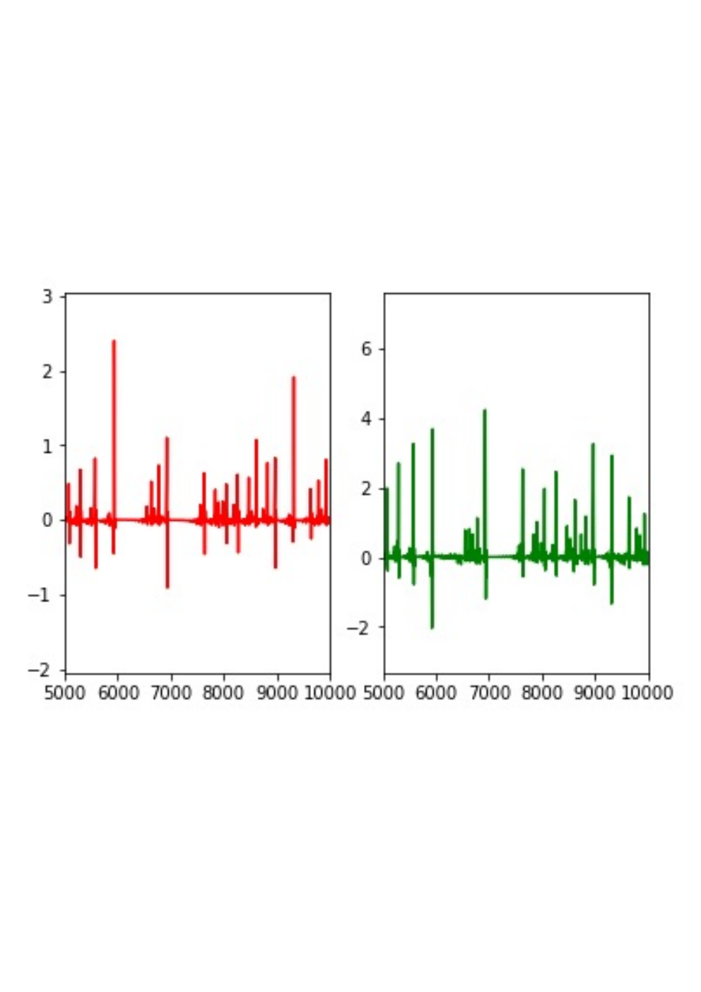
Figure 3.4.7 shows the results for an initial condition and 10,000 points. Figure 3.4.8 shows the prediction errors for the case of an approximation with a learned kernel and a kernel without learning. Figure 3.4.9 shows the projection of the attractor and its approximation with a learned kernel and a kernel without learning. Figure 3.4.10 shows the attractor with a learned kernel and a kernel without learning.




We also consider a parameterized family of kernels of the form
| (20) |
The training and prediction results are shown in the following table with the RMSE corresponding to 50,000 points with initial conditions .
| n | |||
|---|---|---|---|
| 1000 | |||
| 0 |
Remarks
- 1.
- 2.
- 3.
It is possible to include new measurements when approximating the dynamics from data without repeating the learning process. This can be done by working in Newton basis as in [36].
4 Conclusion
Our experiments suggest that using cross-validation (with KF and variants) to learn the kernel used to approximate the vector field of a dynamical system, and thereby its dynamics, significantly improves the accuracy of such approximations. Although our paper is entirely numerical, the simplicity of the proposed approach and the diversity of the experiments raise the question of the existence of a general and fundamental convergence theorem for cross-validation.
5 Acknowledgment
B. H. thanks the European Commission for funding through the Marie Curie fellowship STALDYS-792919 (Statistical Learning for Dynamical Systems). H. O. gratefully acknowledges support by the Air Force Office of Scientific Research under award number FA9550-18-1-0271 (Games for Computation and Learning). We thank Deniz Eroğlu, Yoshito Hirata, Jeroen Lamb, Edmilson Roque, Gabriele Santin and Yuzuru Sato for useful comments.
Appendix A Reproducing Kernel Hilbert Spaces
We give a brief overview of reproducing kernel Hilbert spaces as used in statistical learning theory [16]. Early work developing the theory of RKHS was undertaken by N. Aronszajn [3].
Definition A.1.
Let be a Hilbert space of functions on a set .
Denote by the inner product on and let
be the norm in , for and . We say that is a reproducing kernel
Hilbert space (RKHS) if there exists a function
such that
i. for all .
ii. spans : .
iii. has the reproducing property:
, .
will be called a reproducing kernel of . will denote the RKHS
with reproducing kernel where it is convenient to explicitly note this dependence.
The important properties of reproducing kernels are summarized in the following proposition.
Proposition A.1.
If is a reproducing kernel of a Hilbert space , then
i. is unique.
ii. , (symmetry).
iii. for , and
(positive definiteness).
iv. .
Common examples of reproducing kernels defined on a compact domain are the (1) constant kernel: (2) linear kernel: (3) polynomial kernel: for (4) Laplace kernel: , with (5) Gaussian kernel: , with (6) triangular kernel: , with . (7) locally periodic kernel: , with .
Theorem A.1.
Let be a symmetric and positive definite function. Then there exists a Hilbert space of functions defined on admitting as a reproducing Kernel. Conversely, let be a Hilbert space of functions satisfying such that Then has a reproducing kernel .
Theorem A.2.
Let be a positive definite kernel on a compact domain or a manifold . Then there exists a Hilbert space and a function such that
is called a feature map, and a feature space66 6 The dimension of the feature space can be infinite, for example in the case of the Gaussian kernel..
A.1 Function Approximation in RKHSs: An Optimal Recovery Viewpoint
In this section we review function approximation in RKHSs from the point of view of optimal recovery as discussed in [33].
Problem P:
Given input/output data , recover an unknown function mapping to such that for .
In the setting of optimal recovery [33] Problem P can be turned into a well posed problem by restricting candidates for to belong to a Banach space of functions endowed with a norm and identifying the optimal recovery as the minimizer of the relative error
| (21) |
where the max is taken over and the min is taken over candidates in such that . For the validity of the constraints , , the dual space of , must contain delta Dirac functions . This problem can be stated as a game between Players I and II and can then be represented as
| (22) |
If is quadratic, i.e. where stands for the duality product between and and is a positive symmetric linear bijection (i.e. such that and for ). In that case the optimal solution of (21) has the explicit form
| (23) |
where and is a Gram matrix with entries .
To recover the classical representer theorem, one defines the reproducing kernel as
In this case, can be seen as an RKHS endowed with the norm
and (23) corresponds to the classical representer theorem
| (24) |
using the vectorial notation with , and .
Now, let us consider the problem of learning the kernel from data. As introduced in [31], the method of KFs is based on the premise that a kernel is good if there is no significant loss in accuracy in the prediction error if the number of data points is halved. This led to the introduction of
| (25) |
which is the relative error between , the optimal recovery (24) of based on the full dataset , and the optimal recovery of both and based on half of the dataset () which admits the representation
| (26) |
with , , , . This quantity is directly related to the game in (22) where one is minimizing the relative error of versus . Instead of using the entire the dataset one may use random subsets (of ) for and random subsets (of ) for .
Replacing by the RKHS norm of the interpolant of (with both testing and training points) in (4) gives an error interval for in (24) as
| (27) |
with
| (28) |
and where corresponds to the concatenation of the training and testing points. Local error estimates such as (27) are classical in Kriging [27] (see also [32][Thm. 5.1] for applications to PDEs). .
A.2 The Maximum Mean Discrepancy
Let be the set of Borel probability measures on . Given a probability distribution we define its kernel mean embedding (with respect to a kernel with RKHS ) as
The maximum mean discrepancy (MMD) between two probability measures and is then defined as the distance between two such embeddings and can be expressed as
where and are independent random variables drawn according to , and are independent random variables drawn according to , and is independent of .
Given i.i.d. samples from and , from and respectively, recall that the MMD in RKHSs is defined as the difference between the kernel mean embeddings defined as as follows. Given i.i.d samples from and from , the MMD between the empirical distributions and is an unbiased estimate of with the representation
| (29) |
References
- [1] H. Abarbanel. Analysis of Observed Chaotic Data. Institute for Nonlinear Science. Springer New York, 2012.
- [2] Romeo Alexander and Dimitrios Giannakis. Operator-theoretic framework for forecasting nonlinear time series with kernel analog techniques. Physica D: Nonlinear Phenomena, 409:132520, 2020.
- [3] N. Aronszajn. Theory of reproducing kernels. Transactions of the American Mathematical Society, 68(3):337–404, 1950.
- [4] Andreas Bittracher, Stefan Klus, Boumediene Hamzi, Péter Koltai, and Christof Schütte. Dimensionality reduction of complex metastable systems via kernel embeddings of transition manifolds. 2019. https://arxiv.org/abs/1904.08622.
- [5] J. Bouvrie and B. Hamzi. Balanced reduction of nonlinear control systems in reproducing kernel hilbert space. Proc. 48th Annual Allerton Conference on Communication, Control, and Computing, pages 294–301, 2010. http://arxiv.org/abs/1011.2952.
- [6] J. Bouvrie and B. Hamzi. Balanced reduction of nonlinear control systems in reproducing kernel hilbert space. Proc. of the 2012 American Control Conference, pages 294–301, 2012. http://arxiv.org/abs/1204.0563.
- [7] J. Bouvrie and B. Hamzi. Kernel methods for the approximation of nonlinear systems. SIAM J. Control and Optimization, 2017. https://arxiv.org/abs/1108.2903.
- [8] J. Bouvrie and B. Hamzi. Kernel methods for the approximation of some key quantities of nonlinear systems. Journal of Computational Dynamics, (1), 2017. http://arxiv.org/abs/1204.0563.
- [9] George.E.P. Box and Gwilym M. Jenkins. Time Series Analysis: Forecasting and Control. Holden-Day, 1976.
- [10] Steven L. Brunton, W. Bingni, Joshua L. Proctor, Eurika Kaiser, and J. Nathan Kutz. Chaos as an intermittently forced linear system. Nature Communications, 8(1):19, 2017.
- [11] Steven L. Brunton, Joshua L. Proctor, and J. Nathan Kutz. Discovering governing equations from data by sparse identification of nonlinear dynamical systems. Proceedings of the National Academy of Sciences, 113(15):3932–3937, 2016.
- [12] M. Budišić, R. Mohr, and I. Mezić. The Koopman Operator in Systems and Control: Concepts, Methodologies, and Applications. Springer, 2020.
- [13] Martin Casdagli. Nonlinear prediction of chaotic time series. Physica D: Nonlinear Phenomena, 35(3):335 – 356, 1989.
- [14] Ashesh Chattopadhyay, Pedram Hassanzadeh, Krishna V. Palem, and Devika Subramanian. Data-driven prediction of a multi-scale lorenz 96 chaotic system using a hierarchy of deep learning methods: Reservoir computing, ann, and RNN-LSTM. CoRR, abs/1906.08829, 2019.
- [15] Yifan Chen, Houman Owhadi, and Andrew M. Stuart. Consistency of empirical bayes and kernel flow for hierarchical parameter estimation. 2020. https://arxiv.org/abs/2005.11375.
- [16] Felipe Cucker and Steve Smale. On the mathematical foundations of learning. Bulletin of the American Mathematical Society, 39:1–49, 2002.
- [17] J. P. Eckmann, S. Oliffson Kamphorst, D. Ruelle, and S. Ciliberto. Liapunov exponents from time series. Phys. Rev. A, 34:4971–4979, Dec 1986.
- [18] P. Giesl, B. Hamzi, M. Rasmussen, and K. Webster. Approximation of Lyapunov functions from noisy data. Journal of Computational Dynamics, 2019. https://arxiv.org/abs/1601.01568.
- [19] Arthur Gretton, Karsten M. Borgwardt, Malte J. Rasch, Bernhard Schölkopf, and Alexander Smola. A kernel two-sample test. Journal of Machine Learning Research, 13(25):723–773, 2012.
- [20] B. Haasdonk, B. Hamzi, G. Santin, and D. Wittwar. Greedy kernel methods for center manifold approximation. Proc. of ICOSAHOM 2018, International Conference on Spectral and High Order Methods, (1), 2018. https://arxiv.org/abs/1810.11329.
- [21] Holger Kantz and Thomas Schreiber. Nonlinear Time Series Analysis. Cambridge University Press, USA, 1997.
- [22] S. Klus, F. Nüske, S. Peitz, J.-H. Niemann, C. Clementi, and C. Schütte. Data-driven approximation of the Koopman generator: Model reduction, system identification, and control. Physica D: Nonlinear Phenomena, 406:132416, 2020.
- [23] Stefan Klus, Feliks Nuske, and Boumediene Hamzi. Kernel-based approximation of the koopman generator and schrödinger operator. Entropy, 22, 2020. https://www.mdpi.com/1099-4300/22/7/722.
- [24] Stefan Klus, Feliks Nüske, Sebastian Peitz, Jan-Hendrik Niemann, Cecilia Clementi, and Christof Schütte. Data-driven approximation of the koopman generator: Model reduction, system identification, and control. Physica D: Nonlinear Phenomena, 406:132416, 2020.
- [25] Zhixin Lu, Brian R. Hunt, and Edward Ott. Attractor reconstruction by machine learning. Chaos: An Interdisciplinary Journal of Nonlinear Science, 28(6):061104, 2018.
- [26] W Melo and S Strien. One-Dimensional Dynamics. Springer Berlin Heidelberg, 1993.
- [27] Zong min Wu and Robert Schaback. Local error estimates for radial basis function interpolation of scattered data. IMA J. Numer. Anal, 13:13–27, 1992.
- [28] S. Mukherjee, E. Osuna, and F. Girosi. Nonlinear prediction of chaotic time series using support vector machines. In Neural Networks for Signal Processing VII. Proceedings of the 1997 IEEE Signal Processing Society Workshop, pages 511–520, 1997.
- [29] Klaus-Robert Müller, Alex J. Smola, Gunnar Rätsch, Bernhard Schölkopf, Jens Kohlmorgen, and Vladimir Vapnik. Predicting time series with support vector machines. In Proceedings of the 7th International Conference on Artificial Neural Networks, ICANN ’97, page 999–1004, Berlin, Heidelberg, 1997. Springer-Verlag.
- [30] A. Nielsen. Practical Time Series Analysis: Prediction with Statistics and Machine Learning. O’Reilly Media, 2019.
- [31] H. Owhadi and G. R. Yoo. Kernel flows: From learning kernels from data into the abyss. Journal of Computational Physics, 389:22–47, 2019.
- [32] Houman Owhadi. Bayesian numerical homogenization. Multiscale Modeling & Simulation, 13(3):812–828, 2015.
- [33] Houman Owhadi and Clint Scovel. Operator-Adapted Wavelets, Fast Solvers, and Numerical Homogenization: From a Game Theoretic Approach to Numerical Approximation and Algorithm Design. Cambridge Monographs on Applied and Computational Mathematics. Cambridge University Press, 2019.
- [34] Houman Owhadi, Clint Scovel, and Gene Ryan Yoo. Kernel mode decomposition and programmable/interpretable regression networks. 2019. https://arxiv.org/abs/1907.08592.
- [35] Jaideep Pathak, Zhixin Lu, Brian R. Hunt, Michelle Girvan, and Edward Ott. Using machine learning to replicate chaotic attractors and calculate lyapunov exponents from data. Chaos: An Interdisciplinary Journal of Nonlinear Science, 27(12):121102, 2017.
- [36] Maryam Pazouki and Robert Schaback. Bases for kernel-based spaces. Journal of Computational and Applied Mathematics, 236(4):575 – 588, 2011. International Workshop on Multivariate Approximation and Interpolation with Applications (MAIA 2010).
- [37] Liva Ralaivola and Florence d’Alché Buc. Dynamical modeling with kernels for nonlinear time series prediction. In S. Thrun, L. K. Saul, and B. Schölkopf, editors, Advances in Neural Information Processing Systems 16, pages 129–136. MIT Press, 2004.
- [38] G. Santin and B. Haasdonk. Kernel methods for surrogate modelling. ArXiv e-prints arXiv:1907.10556, 2019. https://arxiv.org/abs/1907.10556.
- [39] Florian Schäfer, Matthias Katzfuss, and Houman Owhadi. Sparse cholesky factorization by kullback-leibler minimization. 2020. https://arxiv.org/abs/2004.14455.
- [40] Christopher Schölzel. Nonlinear measures for dynamical systems, June 2019. https://doi.org/10.5281/zenodo.3814723.
- [41] R.H. Shumway and D.S. Stoffer. Time Series Analysis and Its Applications: With R Examples. Springer Texts in Statistics. Springer New York, 2010.
- [42] Gene Ryan Yoo and Houman Owhadi. Deep regularization and direct training of the inner layers of neural networks with kernel flows. 2020. https://arxiv.org/abs/2002.08335.