跳到论文正文
W Papers独立论文阅读器 arXiv:2007.05004 论文正文 计算阅读时间 · 0%
引用这篇论文根据当前论文元数据生成,正式投稿前建议核对。


License: CC BY 4.0
arXiv:2007.05004v5 [hep-ph] 19 May 2023

Higgs sector phenomenology in the 3-3-1 model with an axionlike particle

V. H. Binha,b Email: vhbinh@iop.vast.vn Affiliation: a Graduate University of Science and Technology, Vietnam Academy of Science and Technology, 18 Hoang Quoc Viet, Cau Giay, Hanoi 10000, Vietnam
b Institute of Physics, Vietnam Academy of Science and Technology, 10 Dao Tan, Ba Dinh, Hanoi 10000, Vietnam
c Institute of Theoretical and Applied Research, Duy Tan University, Hanoi 10000, Vietnam
d Faculty of Natural Science, Duy Tan University, Da Nang 55000, Vietnam
e Universidad Técnica Federico Santa María, Casilla 110-V, Valparaíso, Chile
f Centro Científico-Tecnológico de Valparaíso, Casilla 110-V, Valparaíso, Chile
g Millennium Institute for Subatomic physics at high energy frontier - SAPHIR, Fernandez Concha 700, Santiago, Chile
h Faculty of Applied Sciences, University of Economics and Technology for Industries, 456 Minh Khai, Hai Ba Trung, Hanoi 10000, Vietnam
k Subatomic Physics Research Group, Science and Technology Advanced Institute,
Van Lang University, Ho Chi Minh City 70000, Vietnam
l Faculty of Applied Technology, School of Technology, Van Lang University, Ho Chi Minh City 70000, Vietnam
   D. T. Binhc,d Email: dinhthanhbinh3@duytan.edu.vn Affiliation: a Graduate University of Science and Technology, Vietnam Academy of Science and Technology, 18 Hoang Quoc Viet, Cau Giay, Hanoi 10000, Vietnam
b Institute of Physics, Vietnam Academy of Science and Technology, 10 Dao Tan, Ba Dinh, Hanoi 10000, Vietnam
c Institute of Theoretical and Applied Research, Duy Tan University, Hanoi 10000, Vietnam
d Faculty of Natural Science, Duy Tan University, Da Nang 55000, Vietnam
e Universidad Técnica Federico Santa María, Casilla 110-V, Valparaíso, Chile
f Centro Científico-Tecnológico de Valparaíso, Casilla 110-V, Valparaíso, Chile
g Millennium Institute for Subatomic physics at high energy frontier - SAPHIR, Fernandez Concha 700, Santiago, Chile
h Faculty of Applied Sciences, University of Economics and Technology for Industries, 456 Minh Khai, Hai Ba Trung, Hanoi 10000, Vietnam
k Subatomic Physics Research Group, Science and Technology Advanced Institute,
Van Lang University, Ho Chi Minh City 70000, Vietnam
l Faculty of Applied Technology, School of Technology, Van Lang University, Ho Chi Minh City 70000, Vietnam
   A. E. Cárcamo Hernándeze,f,g Email: antonio.carcamo@usm.cl Affiliation: a Graduate University of Science and Technology, Vietnam Academy of Science and Technology, 18 Hoang Quoc Viet, Cau Giay, Hanoi 10000, Vietnam
b Institute of Physics, Vietnam Academy of Science and Technology, 10 Dao Tan, Ba Dinh, Hanoi 10000, Vietnam
c Institute of Theoretical and Applied Research, Duy Tan University, Hanoi 10000, Vietnam
d Faculty of Natural Science, Duy Tan University, Da Nang 55000, Vietnam
e Universidad Técnica Federico Santa María, Casilla 110-V, Valparaíso, Chile
f Centro Científico-Tecnológico de Valparaíso, Casilla 110-V, Valparaíso, Chile
g Millennium Institute for Subatomic physics at high energy frontier - SAPHIR, Fernandez Concha 700, Santiago, Chile
h Faculty of Applied Sciences, University of Economics and Technology for Industries, 456 Minh Khai, Hai Ba Trung, Hanoi 10000, Vietnam
k Subatomic Physics Research Group, Science and Technology Advanced Institute,
Van Lang University, Ho Chi Minh City 70000, Vietnam
l Faculty of Applied Technology, School of Technology, Van Lang University, Ho Chi Minh City 70000, Vietnam
   D. T. Huongb Email: dthuong@iop.vast.vn Affiliation: a Graduate University of Science and Technology, Vietnam Academy of Science and Technology, 18 Hoang Quoc Viet, Cau Giay, Hanoi 10000, Vietnam
b Institute of Physics, Vietnam Academy of Science and Technology, 10 Dao Tan, Ba Dinh, Hanoi 10000, Vietnam
c Institute of Theoretical and Applied Research, Duy Tan University, Hanoi 10000, Vietnam
d Faculty of Natural Science, Duy Tan University, Da Nang 55000, Vietnam
e Universidad Técnica Federico Santa María, Casilla 110-V, Valparaíso, Chile
f Centro Científico-Tecnológico de Valparaíso, Casilla 110-V, Valparaíso, Chile
g Millennium Institute for Subatomic physics at high energy frontier - SAPHIR, Fernandez Concha 700, Santiago, Chile
h Faculty of Applied Sciences, University of Economics and Technology for Industries, 456 Minh Khai, Hai Ba Trung, Hanoi 10000, Vietnam
k Subatomic Physics Research Group, Science and Technology Advanced Institute,
Van Lang University, Ho Chi Minh City 70000, Vietnam
l Faculty of Applied Technology, School of Technology, Van Lang University, Ho Chi Minh City 70000, Vietnam
   D. V. Soah Email: dvsoa@hnmu.edu.vn Affiliation: a Graduate University of Science and Technology, Vietnam Academy of Science and Technology, 18 Hoang Quoc Viet, Cau Giay, Hanoi 10000, Vietnam
b Institute of Physics, Vietnam Academy of Science and Technology, 10 Dao Tan, Ba Dinh, Hanoi 10000, Vietnam
c Institute of Theoretical and Applied Research, Duy Tan University, Hanoi 10000, Vietnam
d Faculty of Natural Science, Duy Tan University, Da Nang 55000, Vietnam
e Universidad Técnica Federico Santa María, Casilla 110-V, Valparaíso, Chile
f Centro Científico-Tecnológico de Valparaíso, Casilla 110-V, Valparaíso, Chile
g Millennium Institute for Subatomic physics at high energy frontier - SAPHIR, Fernandez Concha 700, Santiago, Chile
h Faculty of Applied Sciences, University of Economics and Technology for Industries, 456 Minh Khai, Hai Ba Trung, Hanoi 10000, Vietnam
k Subatomic Physics Research Group, Science and Technology Advanced Institute,
Van Lang University, Ho Chi Minh City 70000, Vietnam
l Faculty of Applied Technology, School of Technology, Van Lang University, Ho Chi Minh City 70000, Vietnam
   H. N. Longk,l Email: hoangngoclong@vlu.edu.vn (corresponding author) Affiliation: a Graduate University of Science and Technology, Vietnam Academy of Science and Technology, 18 Hoang Quoc Viet, Cau Giay, Hanoi 10000, Vietnam
b Institute of Physics, Vietnam Academy of Science and Technology, 10 Dao Tan, Ba Dinh, Hanoi 10000, Vietnam
c Institute of Theoretical and Applied Research, Duy Tan University, Hanoi 10000, Vietnam
d Faculty of Natural Science, Duy Tan University, Da Nang 55000, Vietnam
e Universidad Técnica Federico Santa María, Casilla 110-V, Valparaíso, Chile
f Centro Científico-Tecnológico de Valparaíso, Casilla 110-V, Valparaíso, Chile
g Millennium Institute for Subatomic physics at high energy frontier - SAPHIR, Fernandez Concha 700, Santiago, Chile
h Faculty of Applied Sciences, University of Economics and Technology for Industries, 456 Minh Khai, Hai Ba Trung, Hanoi 10000, Vietnam
k Subatomic Physics Research Group, Science and Technology Advanced Institute,
Van Lang University, Ho Chi Minh City 70000, Vietnam
l Faculty of Applied Technology, School of Technology, Van Lang University, Ho Chi Minh City 70000, Vietnam
August 11, 2026
Abstract

The scalar sector of the 3-3-1 model with an axionlike particle is studied in detail. In the model under consideration, there are two kinds of scalar fields: the bilepton scalars carrying lepton number two and the ordinary ones without lepton number. We show that there is no mixing among these two kinds of scalar fields. We analyze in detail the C​PCP-odd scalar sector of the model to find the physical fields of the axionlike particle and a pseudoscalar with mass in the range 100 GeV to 1 TeV. The results are different from others which have been published before. The C​PCP-even scalar sector of the model is analyzed as well. The results of our analysis of the scalar sector allow us to accommodate scalar masses in the n100100 GeV-11 TeV region. Furthermore we analyze the implications of the model in several flavor changing neutral decays of the top quark as well as in rare top quark decays. Besides that, the leptonic decays of the SM like Higgs boson as well as the meson oscillations are also analyzed. Our numerical analysis show that the model under consideration is consistent with the experimental constraints imposed by these processes.

pacs
11.30.Fs, 12.15.Ff, 12.60.-i

I Introduction

Nowadays, it is well known that the standard model (SM) has to be extended. Among the extended models of the SM, the versions based on the SU(3)C×SU(3)L×U(1)X\mbox{SU(3)}_{C}\times\mbox{SU(3)}_{L}\times\mbox{U(1)}_{X} gauge group (called 3-3-1 models in short) ppf1; ppf2; ppf3; ppf4; flt1; flt2; flt3; flt4; flt5; flt6 are of interest with the following intriguing features such as the explanation on the number of fermion generations, the electric charge quantization chargeq1; chargeq2, source of C​PCP violation $CP$s1; $CP$s2 as well as the automatic fulfillment pal of the Peccei-Quinn symmetry pq1; pq2. The Peccei-Quin symmetry for the economical 3-3-1 model eco; eco1; eco2; eco3; eco4; eco5 are discussed in Refs. pal2; pal3. The models contain self-interacting dark matter sidm1; sidm2

The models are classified by a parameter β\beta appearing in the electric charge operator

Q=T3+β​T8+X,Q=T_{3}+\beta\,T_{8}+X\,, (1)

where T3T_{3} and T8T_{8} are S​U​(3)LSU(3)_{L} generators, XX is the U​(1)XU(1)_{X} charge. The 3-3-1 model with arbitrary beta is presented in Ref. beta (see also beta2). There are two main versions of the 3-3-1 models. The first one is the minimal model with β=±3\beta=\pm\sqrt{3} which requires three S​U​(3)LSU(3)_{L} scalar triplets and one S​U​(3)LSU(3)_{L} scalar sextet ppf1; ppf2; ppf3. Moreover, this version has a Landau pole around 5 TeV leading to a loss of pertubartivity around that scale. There exists effort to solve this puzzle mimln. In the recent work mimlp, the Landau pole, in the minimal version by addition of octet leptoquarks, can be around 100 TeV. The second one is the model with β=±13\beta=\pm\frac{1}{\sqrt{3}} which just requires three S​U​(3)LSU(3)_{L} scalar triplets to provide masses for all fermions and bosons flt1; flt2; flt3; flt4; flt5. This kind of model is more attractive due to its simpler scalar content and its lack of Landau pole at the TeV scale.

About two decades ago, the axion have been introduced in the 3-3-1 models a1; a2; a3. The new nice property of the 3-3-1 model is found in a recent paper jpf, where the cosmological inflation, axionlike particle (ALP) and seesaw mechanism are simultaneously addressed with a minimal scalar content. However, the above-mentioned paper contains some mistakes and does not address phenomenological aspects related with flavor changing neutral process such as the t→h​ut\rightarrow hu, t→h​ct\rightarrow hc, t→u​γt\rightarrow u\gamma and t→c​γt\rightarrow c\gamma decays as well as the K0−K¯0K^{0}-\bar{K}^{0}, Bd0−B¯d0B_{d}^{0}-\bar{B}_{d}^{0} and Bs0−B¯s0B_{s}^{0}-\bar{B}_{s}^{0} meson oscillations whose explanations, analysis and discussions are the purpose of this work.

II Brief review of the model

II.1 Particle content and discrete symmetries

To provide masses for fermions and to account for the existence of the ALP, the scalar sector of the model requires three S​U​(3)LSU(3)_{L} scalar triplets η,ρ,χ\eta,\rho,\chi as well as an electrically neutral S​U​(3)LSU(3)_{L} scalar singlet ϕ\phi. The scalar content of the model with their corresponding SU(3)C×SU(3)L×U(1)X\mbox{SU(3)}_{C}\times\mbox{SU(3)}_{L}\times\mbox{U(1)}_{X} assignments are given by:

χT\displaystyle\chi^{T} =\displaystyle= (χ10,χ2−,χ30)∼(1,3,−13),ηT=(η10,η2−,η30)∼(1,3,−13),\displaystyle\left(\chi^{0}_{1},\chi^{-}_{2},\chi_{3}^{0}\right)\sim\left(1,3,-\frac{1}{3}\right),\,\eta^{T}=\left(\eta^{0}_{1},\eta^{-}_{2},\eta_{3}^{0}\right)\sim\left(1,3,-\frac{1}{3}\right),
ρT\displaystyle\rho^{T} =\displaystyle= (ρ1+,ρ20,ρ3+)∼(1,3,23),ϕ∼(1,1,0).\displaystyle\left(\rho^{+}_{1},\rho_{2}^{0},\rho_{3}^{+}\right)\sim\left(1,3,\frac{2}{3}\right),\,\hskip 8.5359pt\phi\sim(1,1,0)\,. (2)

To provide masses for the fermions and gauge bosons, the above scalar fields have vacuum expectation values (VEVs) as follows

⟨χ⟩\displaystyle\langle\chi\rangle =\displaystyle= 12​(0,0,vχ)T,⟨η⟩=12​(vη,0,0)T\displaystyle\frac{1}{\sqrt{2}}\left(0,0,v_{\chi}\right)^{T},\,\hskip 8.5359pt\langle\eta\rangle=\frac{1}{\sqrt{2}}\,\left(v_{\eta},0,0\right)^{T}
⟨ρ⟩\displaystyle\langle\rho\rangle =\displaystyle= 12​(0,vρ,0)T,⟨ϕ⟩=12​vϕ.\displaystyle\frac{1}{\sqrt{2}}\,\left(0,v_{\rho},0\right)^{T},\,\hskip 8.5359pt\langle\phi\rangle=\frac{1}{\sqrt{2}}\,v_{\phi}\,. (3)

where the VEV vχv_{\chi} triggers the spontaneous breaking of the S​U​(3)L×U​(1)XSU(3)_{L}\times U(1)_{X} gauge symmetry down to the SM electroweak gauge group. The remaining S​U​(3)LSU(3)_{L} scalar triplets η\eta and ρ\rho break the SM electroweak gauge group.

On the other hand, the fermion spectrum of the model and their SU(3)C×SU(3)L×U(1)X\mbox{SU(3)}_{C}\times\mbox{SU(3)}_{L}\times\mbox{U(1)}_{X} assignments are:

ψa​L=(νa,ea,(νRc)a)LT∼(1,3,−1/3),ea​R∼(1,1,−1),\displaystyle\psi_{aL}=\left(\nu_{a},e_{a},(\nu^{c}_{R})^{a}\right)_{L}^{T}\sim\left(1,3,-1/3\right),\hskip 8.5359pte_{aR}\sim\left(1,1,-1\right),
Na​R∼(1,1,0),Q3​L=(u3,d3,U)LT∼(3,3,1/3),\displaystyle N_{aR}\sim(1,1,0),Q_{3L}=\left(u_{3},d_{3},U\right)_{L}^{T}\sim\left(3,3,1/3\right),
Qn​L=(dn,−un,Dn)LT∼(3,3∗,0),\displaystyle Q_{nL}=\left(d_{n},-u_{n},D_{n}\right)_{L}^{T}\sim\left(3,3^{\ast},0\right),
ua​R,UR∼(3,1,2/3),da​R,Dn​R∼(3,1,−1/3),\displaystyle u_{aR},U_{R}\sim\left(3,1,2/3\right),\hskip 8.5359ptd_{aR},D_{nR}\sim(3,1,-1/3), (4)

where n=1,2n=1,2 and a={n,3}a=\{n,3\} are family indices. The UU and DD are exotic quarks with ordinary electric charges, whereas Na​RN_{aR} are right-handed Majorana neutrinos.

The typical trouble of the 3-3-1 model with β=±13\beta=\pm\frac{1}{\sqrt{3}} is that there are two triplets η\eta and χ\chi with identical quantum numbers by SU(3)L×U(1)X\mbox{SU(3)}_{L}\times\mbox{U(1)}_{X} gauge group leading to the term μη​χ2​η†​χ\mu^{2}_{\eta\chi}\eta^{\dagger}\chi, which complicates the structure of the square scalar mass matrices, thus making the analysis of the scalar sector very tedious. To avoid this kind of terms, one imposes the Z2Z_{2} discrete symmetry under which the S​U​(3)LSU(3)_{L} scalar triplets η\eta and χ\chi have opposite numbers, as done in Ref.a2. To provide Dirac and Majorana mass terms for νL\nu_{L} and NRN_{R} we have the above described particle content, shown in Table 1. The particle assignments under the SU(3)C×SU(3)L×U(1)X×Z11×Z2\mbox{SU(3)}_{C}\times\mbox{SU(3)}_{L}\times\mbox{U(1)}_{X}\times Z_{11}\times Z_{2} group are summarized in Table 1. Here we have used a notation ωk≡ei​2​π​k11,k=0,±1⋯±5\omega_{k}\equiv e^{i2\pi\frac{k}{11}},k=0,\pm 1\cdots\pm 5.

Qn​LQ_{nL} Q3​LQ_{3L} ua​Ru_{aR} da​Rd_{aR} U3​RU_{3R} Dn​RD_{nR} ψa​L\psi_{aL} ea​Re_{aR} Na​RN_{aR} η\eta χ\chi ρ\rho ϕ\phi
S​U​(3)CSU(3)_{C} 𝟑\mathbf{3} 𝟑\mathbf{3} 𝟑\mathbf{3} 𝟑\mathbf{3} 𝟑\mathbf{3} 𝟑\mathbf{3} 𝟏\mathbf{1} 𝟏\mathbf{1} 𝟏\mathbf{1} 𝟏\mathbf{1} 𝟏\mathbf{1} 𝟏\mathbf{1} 𝟏\mathbf{1}
S​U​(3)LSU(3)_{L} 𝟑¯\overline{\mathbf{3}} 𝟑\mathbf{3} 𝟏\mathbf{1} 𝟏\mathbf{1} 𝟏\mathbf{1} 𝟏\mathbf{1} 𝟑\mathbf{3} 𝟏\mathbf{1} 𝟏\mathbf{1} 𝟑\mathbf{3} 𝟑\mathbf{3} 𝟑\mathbf{3} 𝟏\mathbf{1}
U​(1)XU(1)_{X} 00 13\frac{1}{3} 23\frac{2}{3} −13-\frac{1}{3} 23\frac{2}{3} −13-\frac{1}{3} −13-\frac{1}{3} −1-1 00 −13-\frac{1}{3} −13-\frac{1}{3} 23\frac{2}{3} 00
Z11Z_{11} ω4−1\omega^{-1}_{4} ω0\omega_{0} ω5\omega_{5} ω2\omega_{2} ω3\omega_{3} ω4\omega_{4} ω1\omega_{1} ω3\omega_{3} ω5−1\omega^{-1}_{5} ω5−1\omega^{-1}_{5} ω3−1\omega^{-1}_{3} ω2−1\omega^{-1}_{2} ω1−1\omega^{-1}_{1}
Z2Z_{2} 11 11 −1-1 −1-1 11 11 11 −1-1 −1-1 −1-1 11 −1-1 11
Table 1: S​U​(3)C×S​U​(3)L×U​(1)X×Z11×Z2SU(3)_{C}\times SU(3)_{L}\times U(1)_{X}\times Z_{11}\times Z_{2} charge assignments of the particle content of the model. Here a=1,2,3a=1,2,3 and α=1,2\alpha=1,2.

From Table 1, one recognizes that under Z2Z_{2} symmetry, the following fields are odd

(η,ρ,uR,dn​R,en​R,NR)→−(η,ρ,uR,dn​R,en​R,NR).(\eta\,,\rho\,,u_{R}\,,d_{nR},e_{nR},N_{R})\,\,\,\,\rightarrow\,\,\,\,-\,(\eta\,,\rho\,,u_{R}\,,d_{nR},e_{nR},N_{R})\,. (5)

II.2 Yukawa couplings

With the above specified particle content, the following Yukawa interactions invariant under the S​U​(3)C×S​U​(3)L×U​(1)X×Z11×Z2SU(3)_{C}\times SU(3)_{L}\times U(1)_{X}\times Z_{11}\times Z_{2} symmetry, arise jpf:

−ℒY\displaystyle-\mathcal{L}^{Y} =\displaystyle= y1​Q¯3​L​UR​χ+∑n,m=12(y2)n,m​Q¯n​L​Dm​R​χ∗\displaystyle y_{1}\bar{Q}_{3L}U_{R}\chi+\sum\limits_{n,m=1}^{2}\left(y_{2}\right)_{n,m}\bar{Q}_{nL}D_{mR}\chi^{\ast} (6)
+∑a=13(y3)3​aQ¯3​Lua​Rη+∑n=12∑a=13(y4)n​aQ¯n​Lda​Rη∗\displaystyle+\sum\limits_{a=1}^{3}\left(y_{3}\right)_{3a}\bar{Q}_{3L}u_{aR}\eta+\sum\limits_{n=1}^{2}\sum\limits_{a=1}^{3}\left(y_{4}\right)_{na}\bar{Q}_{nL}d_{aR}\eta^{\ast}
+∑a=13(y5)3​aQ¯3​Lda​Rρ+∑n=12∑a=13(y6)n​aQ¯n​Lua​Rρ∗\displaystyle+\sum\limits_{a=1}^{3}\left(y_{5}\right)_{3a}\bar{Q}_{3L}d_{aR}\rho+\sum\limits_{n=1}^{2}\sum\limits_{a=1}^{3}\left(y_{6}\right)_{na}\bar{Q}_{nL}u_{aR}\rho^{\ast}
+∑a=13∑b=13ga​bψ¯a​Leb​Rρ+∑a=13∑b=13(yνD)a​bψ¯a​LηNb​R\displaystyle+\sum\limits_{a=1}^{3}\sum\limits_{b=1}^{3}g_{ab}\bar{\psi}_{aL}e_{bR}\rho+\sum\limits_{a=1}^{3}\sum\limits_{b=1}^{3}\left(y_{\nu}^{D}\right)_{ab}\bar{\psi}_{aL}\eta N_{bR}
+∑a=13∑b=13(yN)a​bϕN¯a​RCNb​R+H.c..\displaystyle+\sum\limits_{a=1}^{3}\sum\limits_{b=1}^{3}\left(y_{N}\right)_{ab}\phi\bar{N}_{aR}^{C}N_{bR}+\mbox{H.c.}.

Let us note that the above given Yukawa interactions in (6) are invariant only under the Z2Z_{2} assignment given above. It is emphasized that the transformation under the Z2Z_{2} in this paper is different from than the one given in Ref. jpf where χ\chi is odd.

The exotic quarks get masses from vχv_{\chi}, top quark get mass from vηv_{\eta}, charged leptons get masses from vρv_{\rho}, while new Majorana neutrino NRN_{R} gets mass through vϕv_{\phi}. The Dirac neutrino mass term arises from vηv_{\eta}, while the Majorana mass term arises from vϕv_{\phi} (see last two terms in (6)). From the last two terms of Eq. (6), it follows that the tiny masses for the light active neutrinos are generated from a type I seesaw mechanism mediated by right handed Majorana neutrinos, thus implying that the resulting light active neutrino mass matrix has the form:

Mν=MνD​MN−1​(MνD)T,MνD=yνD​vη2,MN=2​yN​vϕ.M_{\nu}=M^{D}_{\nu}M^{-1}_{N}\left(M^{D}_{\nu}\right)^{T},\hskip 8.5359ptM^{D}_{\nu}=y^{D}_{\nu}\frac{v_{\eta}}{\sqrt{2}},\hskip 8.5359ptM_{N}=\sqrt{2}\,y_{N}v_{\phi}. (7)

II.3 Gauge bosons

First of all, the model has nine electroweak gauge bosons arising from the S​U​(3)L×U​(1)XSU(3)_{L}\times U(1)_{X} symmetry. Their interactions with the S​U​(3)LSU(3)_{L} scalar triplets are included in the following kinetic terms:

ℒH​i​g​g​s=∑H=χ,η,ρ,ϕ(Dμ​H)†​Dμ​H,\mathcal{L}_{Higgs}=\sum_{H=\chi,\eta,\rho,\phi}(D^{\mu}H)^{\dagger}D_{\mu}H\,, (8)

where the covariant derivative is given by

Dμ≡∂μ−igTaWaμ−igXXT9Xμ,D_{\mu}\equiv\partial_{\mu}-igT^{a}W^{a}_{\mu}-ig_{X}XT^{9}X_{\mu}, (9)

where T9=1/6​I3×3T^{9}=1/\sqrt{6}I_{3\times 3} being I3×3I_{3\times 3} the 3×33\times 3 identity matrix and gg, gXg_{X} are gauge couplings of the two groups S​U​(3)LSU(3)_{L} and U​(1)XU(1)_{X}, respectively. Secondly, the matrix Wa​TaW^{a}T^{a}, where Ta=λa/2T^{a}=\lambda_{a}/2 corresponds to a triplet representation, is written as follows:

Wμa​Ta=12​(Wμ3+13​Wμ82​Wμ+2​Yμ+2​Wμ−−Wμ3+13​Wμ82​Xμ02​Yμ−2X0∗μ−23​Wμ8),\displaystyle W^{a}_{\mu}T^{a}=\frac{1}{2}\left(\begin{array}[]{ccc}W^{3}_{\mu}+\frac{1}{\sqrt{3}}W^{8}_{\mu}&\sqrt{2}W^{+}_{\mu}&\sqrt{2}Y^{+}_{\mu}\\ \sqrt{2}W^{-}_{\mu}&-W^{3}_{\mu}+\frac{1}{\sqrt{3}}W^{8}_{\mu}&\sqrt{2}X^{0}_{\mu}\\ \sqrt{2}Y^{-}_{\mu}&\sqrt{2}X^{0*}_{\mu}&-\frac{2}{\sqrt{3}}W^{8}_{\mu}\\ \end{array}\right),

in which we have defined the mass eigenstates of the charged gauge bosons as

Wμ±\displaystyle W^{\pm}_{\mu} =\displaystyle= 12​(Wμ1∓i​Wμ2),\displaystyle\frac{1}{\sqrt{2}}\left(W^{1}_{\mu}\mp iW^{2}_{\mu}\right),
Yμ±\displaystyle Y^{\pm}_{\mu} =\displaystyle= 12(Wμ4∓iWμ5),Xμ0=12(Wμ6−iWμ7),Xμ0∗=12(Wμ6+iWμ7).\displaystyle\frac{1}{\sqrt{2}}\left(W^{4}_{\mu}\mp iW^{5}_{\mu}\right),\hskip 8.5359ptX^{0}_{\mu}=\frac{1}{\sqrt{2}}\left(W^{6}_{\mu}-iW^{7}_{\mu}\right),\hskip 8.5359ptX^{0*}_{\mu}=\frac{1}{\sqrt{2}}\left(W^{6}_{\mu}+iW^{7}_{\mu}\right). (14)

After spontaneous symmetry breaking, the mass spectrum of the gauge bosons arise from the following terms:

ℒm​a​s​s=∑H=χ,η,ρ(Dμ​⟨H⟩)†​(Dμ​⟨H⟩).\mathcal{L}_{mass}=\sum_{H=\chi,\eta,\rho}(D^{\mu}\langle H\rangle)^{\dagger}(D_{\mu}\langle H\rangle)\,. (15)

The charged and bilepton gauge bosons get masses given by:

mW2=g24​(vη2+vρ2),mX02=g24​(vχ2+vη2),mY2=g24​(vχ2+vρ2).m^{2}_{W}=\frac{g^{2}}{4}(v_{\eta}^{2}+v_{\rho}^{2}),\hskip 8.5359ptm^{2}_{X^{0}}=\frac{g^{2}}{4}(v_{\chi}^{2}+v_{\eta}^{2}),\hskip 8.5359ptm^{2}_{Y}=\frac{g^{2}}{4}(v_{\chi}^{2}+v_{\rho}^{2})\,. (16)

WW is identical to that of the standard model, while (X,Y)(X,Y) form a new, heavy gauge vector doublet with a mass splitting il

|mY2−mX02|<mW2.|m^{2}_{Y}-m^{2}_{X^{0}}|<m^{2}_{W}\,.

From (16), it follows

vη2+vρ2=ve​w2=2462​GeV2.v_{\eta}^{2}+v_{\rho}^{2}=v_{ew}^{2}=246^{2}\,\textrm{GeV}^{2}\,. (17)

Finally, there is a mixing among the W3,W8,BW_{3},W_{8},B components. In the basis of these elements, the mass matrix is given by

Mn​e​u​r​a​l2=g24​(vη2+vρ2vη2−vρ23−2​t3​6​(vη2+2​vρ2)vη2−vρ2313​(4​vχ2+vη2+vρ2)2​t9​(2​vχ2−vη2+2​vρ2)−2​t3​6​(vη2+2​vρ2)2​t9​(2​vχ2−vη2+2​vρ2)2​t227​(vχ2+vη2+4​vρ2)),M_{neural}^{2}=\frac{g^{2}}{4}\left(\begin{array}[]{ccc}v_{\eta}^{2}+v_{\rho}^{2}&\frac{v_{\eta}^{2}-v_{\rho}^{2}}{\sqrt{3}}&-\frac{2t}{3\sqrt{6}}(v_{\eta}^{2}+2v_{\rho}^{2})\\ \frac{v_{\eta}^{2}-v_{\rho}^{2}}{\sqrt{3}}&\frac{1}{3}(4v_{\chi}^{2}+v_{\eta}^{2}+v_{\rho}^{2})&\frac{\sqrt{2}t}{9}(2v_{\chi}^{2}-v_{\eta}^{2}+2v_{\rho}^{2})\\ -\frac{2t}{3\sqrt{6}}(v_{\eta}^{2}+2v_{\rho}^{2})&\frac{\sqrt{2}t}{9}(2v_{\chi}^{2}-v_{\eta}^{2}+2v_{\rho}^{2})&\frac{2t^{2}}{27}(v_{\chi}^{2}+v_{\eta}^{2}+4v_{\rho}^{2})\\ \end{array}\right), (18)

where

t=3​2​sW3−4​sW2.t=\frac{3\sqrt{2}s_{W}}{\sqrt{3-4s^{2}_{W}}}. (19)

Diagonalization proceeds through two steps, in the first step the 3×33\times 3 matrix reduces to one block diagonalized which yields a 2×22\times 2 matrix in the bottom. The eigenstates are now rewritten as follows

Aμ\displaystyle A_{\mu} =\displaystyle= sW​W3​μ+cW​(−tW3​W8​μ+1−tW23​Bμ),\displaystyle s_{W}W_{3\mu}+c_{W}\left(-\frac{t_{W}}{\sqrt{3}}W_{8\mu}+\sqrt{1-\frac{t^{2}_{W}}{3}}B_{\mu}\right),
Zμ\displaystyle Z_{\mu} =\displaystyle= cW​W3​μ−sW​(−tW3​W8​μ+1−tW23​Bμ),\displaystyle c_{W}W_{3\mu}-s_{W}\left(-\frac{t_{W}}{\sqrt{3}}W_{8\mu}+\sqrt{1-\frac{t^{2}_{W}}{3}}B_{\mu}\right),
Zμ′\displaystyle Z^{\prime}_{\mu} =\displaystyle= 1−tW23​W8​μ+tW3​Bμ.\displaystyle\sqrt{1-\frac{t^{2}_{W}}{3}}W_{8\mu}+\frac{t_{W}}{\sqrt{3}}B_{\mu}. (20)

From the analysis of the gauge sector, we found one massless gauge boson, which corresponds to the photon AA. Furthermore, besides the bilepton gauge bosons, the neutral gauge boson spectrum contains two massive neutral gauge bosons ZZ and Z′Z^{\prime}. The elements of the neutral squared gauge boson mass matrix in the (Z,Z′)(Z,Z^{\prime}) basis is given by

mZ2\displaystyle m^{2}_{Z} =\displaystyle= g24​cW2​(vρ2+vη2),\displaystyle\frac{g^{2}}{4c^{2}_{W}}(v_{\rho}^{2}+v_{\eta}^{2}), (21)
mZ​Z′2\displaystyle m^{2}_{ZZ^{\prime}} =\displaystyle= g2​[(tW2−1)​vρ2+(tW2+1)​vη2]4​3​cW​1−13​tW2,\displaystyle\frac{g^{2}\left[(t^{2}_{W}-1)v_{\rho}^{2}+(t^{2}_{W}+1)v_{\eta}^{2}\right]}{4\sqrt{3}c_{W}\sqrt{1-\frac{1}{3}t^{2}_{W}}}, (22)
mZ′2\displaystyle m^{2}_{Z^{\prime}} =\displaystyle= g2​[4​vχ2+(tW2−1)2​vρ2+(tW2+1)2​vη2]4​(3−tW2).\displaystyle\frac{g^{2}\left[4v_{\chi}^{2}+(t^{2}_{W}-1)^{2}v_{\rho}^{2}+(t^{2}_{W}+1)^{2}v_{\eta}^{2}\right]}{4(3-t^{2}_{W})}\,. (23)

Finally, this matrix is diagonalized by the following field transformations

Zμ1\displaystyle Z^{1}_{\mu} =\displaystyle= cθZ​𝒵μ−sθZ​𝒵μ′,\displaystyle c_{\theta_{Z}}{\mathcal{Z}}_{\mu}-s_{\theta_{Z}}\mathcal{Z}^{\prime}_{\mu},
Zμ2\displaystyle Z^{2}_{\mu} =\displaystyle= sθZ​𝒵μ+cθZ​𝒵μ′\displaystyle s_{\theta_{Z}}{\mathcal{Z}}_{\mu}+c_{\theta_{Z}}\mathcal{Z}^{\prime}_{\mu}\, (24)

where Aoidong

t2​θZ\displaystyle t_{2\theta_{Z}} =\displaystyle= sθZcθZ=2​mZ​Z′2mZ′2−mZ2≃(3−tW2)​[(tW2−1)​vρ2+(tW2+1)​vη2]2​vχ2​cW,\displaystyle\frac{s_{\theta_{Z}}}{c_{\theta_{Z}}}=\frac{2m^{2}_{ZZ^{\prime}}}{m^{2}_{Z^{\prime}}-m^{2}_{Z}}\simeq\frac{\sqrt{(3-t^{2}_{W})}\left[(t^{2}_{W}-1)v_{\rho}^{2}+(t^{2}_{W}+1)v_{\eta}^{2}\right]}{2v_{\chi}^{2}c_{W}}, (25)
mZ12\displaystyle m^{2}_{Z_{1}} =\displaystyle= 12​[mZ2+mZ′2−(mZ2−mZ′2)2+4​mZ​Z′4]≃mZ2−mZ​Z′4mZ′2\displaystyle\frac{1}{2}\left[m^{2}_{Z}+m^{2}_{Z^{\prime}}-\sqrt{(m^{2}_{Z}-m^{2}_{Z^{\prime}})^{2}+4m^{4}_{ZZ^{\prime}}}\right]\simeq m^{2}_{Z}-\frac{m^{4}_{ZZ^{\prime}}}{m^{2}_{Z^{\prime}}}
≃\displaystyle\simeq g24​cW2​{vρ2+vη2−[(tW2−1)​vρ2+(tW2+1)​vη2]24​vχ2}≈mW2cW2,\displaystyle\frac{g^{2}}{4c^{2}_{W}}\left\{v_{\rho}^{2}+v_{\eta}^{2}-\frac{\left[(t^{2}_{W}-1)v_{\rho}^{2}+(t^{2}_{W}+1)v_{\eta}^{2}\right]^{2}}{4v_{\chi}^{2}}\right\}\approx\frac{m_{W}^{2}}{c^{2}_{W}},
mZ22\displaystyle m^{2}_{Z_{2}} =\displaystyle= 12​[mZ2+mZ′2+(mZ2−mZ′2)2+4​mZ​Z′4]≃mZ′2≈g2​cW2(3−4​sW2)​vχ2.\displaystyle\frac{1}{2}\left[m^{2}_{Z}+m^{2}_{Z^{\prime}}+\sqrt{(m^{2}_{Z}-m^{2}_{Z^{\prime}})^{2}+4m^{4}_{ZZ^{\prime}}}\right]\simeq m^{2}_{Z^{\prime}}\approx\frac{g^{2}c^{2}_{W}}{(3-4s_{W}^{2})}v_{\chi}^{2}. (26)

Note that exotic quarks UU and DαD_{\alpha} as well as gauge bosons X0,Y±X^{0},Y^{\pm} carry lepton number two joshi; cl; jh18. The gauge boson couplings of this model are the same in Refs. self1; self2. Due to quark family discrimination, there are flavor changing neutral currents mediated by Z′Z^{\prime} at the tree level fc1; fc2; fc3; lv.

III Higgs potential

The model scalar potential has the form:

V\displaystyle V =\displaystyle= μϕ2​ϕ∗​ϕ+μχ2​χ†​χ+μρ2​ρ†​ρ+μη2​η†​η+λ1​(χ†​χ)2+λ2​(η†​η)2\displaystyle\mu^{2}_{\phi}\phi^{*}\phi+\mu_{\chi}^{2}\chi^{\dagger}\chi+\mu_{\rho}^{2}\rho^{\dagger}\rho+\mu_{\eta}^{2}\eta^{\dagger}\eta+\lambda_{1}(\chi^{\dagger}\chi)^{2}+\lambda_{2}(\eta^{\dagger}\eta)^{2} (27)
+λ3​(ρ†​ρ)2+λ4​(χ†​χ)​(η†​η)+λ5​(χ†​χ)​(ρ†​ρ)+λ6​(η†​η)​(ρ†​ρ)\displaystyle+\lambda_{3}(\rho^{\dagger}\rho)^{2}+\lambda_{4}(\chi^{\dagger}\chi)(\eta^{\dagger}\eta)+\lambda_{5}(\chi^{\dagger}\chi)(\rho^{\dagger}\rho)+\lambda_{6}(\eta^{\dagger}\eta)(\rho^{\dagger}\rho)
+λ7​(χ†​η)​(η†​χ)+λ8​(χ†​ρ)​(ρ†​χ)+λ9​(η†​ρ)​(ρ†​η)\displaystyle+\lambda_{7}(\chi^{\dagger}\eta)(\eta^{\dagger}\chi)+\lambda_{8}(\chi^{\dagger}\rho)(\rho^{\dagger}\chi)+\lambda_{9}(\eta^{\dagger}\rho)(\rho^{\dagger}\eta)
+λ10​(ϕ∗​ϕ)2+λ11​(ϕ∗​ϕ)​(χ†​χ)+λ12​(ϕ∗​ϕ)​(ρ†​ρ)\displaystyle+\lambda_{10}(\phi^{*}\phi)^{2}+\lambda_{11}(\phi^{*}\phi)(\chi^{\dagger}\chi)+\lambda_{12}(\phi^{*}\phi)(\rho^{\dagger}\rho)
+λ13(ϕ∗ϕ)(η†η)+(λϕϵi​j​kηiρjχkϕ+H.c.)\displaystyle+\lambda_{13}(\phi^{*}\phi)(\eta^{\dagger}\eta)+\left(\lambda_{\phi}\epsilon^{ijk}\eta_{i}\rho_{j}\chi_{k}\phi+H.c.\right)

The VEV vϕv_{\phi} is responsible for the PQ symmetry breaking resulting in the existence of invisible ALP due to very high scale around 1010−101110^{10}-10^{11} GeV. Then SU(3)L×U(1)X\mbox{SU(3)}_{L}\times\mbox{U(1)}_{X} breaks to the SM group by vχv_{\chi} and two others vρ,vηv_{\rho},v_{\eta} are needed for the usual U(1)Q\mbox{U(1)}_{Q} symmetry. Hence vϕ≫vχ≫vρ,vηv_{\phi}\gg v_{\chi}\gg v_{\rho},v_{\eta}. The constraint conditions of such scalar potential were analyzed in Ref. a2. From (27), it is reasonable to assume: λ2≈λ3,λ4≈λ5,λ7≈λ8,λ12≈λ13\lambda_{2}\approx\lambda_{3},\,\lambda_{4}\approx\lambda_{5},\,\lambda_{7}\approx\lambda_{8},\,\lambda_{12}\approx\lambda_{13}. According Ref. padax, vχ≥10357v_{\chi}\geq 10357 GeV for MZ′≥4.1M_{Z^{\prime}}\geq 4.1 TeV.

Let us expand these scalar fields around their VEVs.

ρ20\displaystyle\rho_{2}^{0} =\displaystyle= 12​(vρ+Rρ+i​Iρ),η10=12​(vη+Rη1+i​Iη1),\displaystyle\frac{1}{\sqrt{2}}(v_{\rho}+R_{\rho}+iI_{\rho})\,,\hskip 8.5359pt\eta_{1}^{0}=\frac{1}{\sqrt{2}}(v_{\eta}+R^{1}_{\eta}+iI^{1}_{\eta})\,,
χ30\displaystyle\chi_{3}^{0} =\displaystyle= 12​(vχ+Rχ3+i​Iχ3),ϕ=12​(vϕ+Rϕ+i​Iϕ).\displaystyle\frac{1}{\sqrt{2}}(v_{\chi}+R^{3}_{\chi}+iI^{3}_{\chi})\,,\hskip 8.5359pt\phi=\frac{1}{\sqrt{2}}(v_{\phi}+R_{\phi}+iI_{\phi})\,. (28)

Substitution of (28) into (27) leads to the following constraints at the tree level as follows

μρ2+λ3​vρ2+λ52​vχ2+λ62​vη2+λ122​vϕ2+A2​vρ2\displaystyle\mu^{2}_{\rho}+\lambda_{3}v_{\rho}^{2}+\frac{\lambda_{5}}{2}v_{\chi}^{2}+\frac{\lambda_{6}}{2}v_{\eta}^{2}+\frac{\lambda_{12}}{2}v_{\phi}^{2}+\frac{A}{2v_{\rho}^{2}} =\displaystyle= 0,\displaystyle 0\,,
μη2+λ2​vη2+λ42​vχ2+λ62​vρ2+λ132​vϕ2+A2​vη2\displaystyle\mu^{2}_{\eta}+\lambda_{2}v_{\eta}^{2}+\frac{\lambda_{4}}{2}v_{\chi}^{2}+\frac{\lambda_{6}}{2}v_{\rho}^{2}+\frac{\lambda_{13}}{2}v_{\phi}^{2}+\frac{A}{2v_{\eta}^{2}} =\displaystyle= 0,\displaystyle 0\,,
μχ2+λ1​vχ2+λ42​vη2+λ52​vρ2+λ112​vϕ2+A2​vχ2\displaystyle\mu^{2}_{\chi}+\lambda_{1}v_{\chi}^{2}+\frac{\lambda_{4}}{2}v_{\eta}^{2}+\frac{\lambda_{5}}{2}v_{\rho}^{2}+\frac{\lambda_{11}}{2}v_{\phi}^{2}+\frac{A}{2v_{\chi}^{2}} =\displaystyle= 0,\displaystyle 0\,,
μϕ2+λ10​vϕ2+λ112​vχ2+λ122​vρ2+λ132​vη2+A2​vϕ2\displaystyle\mu^{2}_{\phi}+\lambda_{10}v_{\phi}^{2}+\frac{\lambda_{11}}{2}v_{\chi}^{2}+\frac{\lambda_{12}}{2}v_{\rho}^{2}+\frac{\lambda_{13}}{2}v_{\eta}^{2}+\frac{A}{2v_{\phi}^{2}} =\displaystyle= 0,\displaystyle 0\,, (29)

where A≡λϕ​vϕ​vχ​vη​vρA\equiv\lambda_{\phi}v_{\phi}v_{\chi}v_{\eta}v_{\rho}.

III.1 Charged scalar sector

There are four charged scalar fields: η2−,ρ1−,ρ3−\eta_{2}^{-},\rho_{1}^{-},\rho_{3}^{-} and χ2−\chi_{2}^{-}.

i) In the basis (η2−,ρ1−\eta_{2}^{-},\rho_{1}^{-}), the corresponding squared mass matrix is given by:

Mc=(λ9​vρ22−A2​vη2λ9​vρ​vη2−A2​vρ​vηλ9​vρ​vη2−A2​vρ​vηλ9​vη22−A2​vρ2)=−(A−λ9​vρ2​vη2)2​(1vη21vη​vρ1vη​vρ1vρ2).M_{c}=\left(\begin{array}[]{cc}\frac{\lambda_{9}v_{\rho}^{2}}{2}-\frac{A}{2v^{2}_{\eta}}&\frac{\lambda_{9}v_{\rho}v_{\eta}}{2}-\frac{A}{2v_{\rho}v_{\eta}}\\ \frac{\lambda_{9}v_{\rho}v_{\eta}}{2}-\frac{A}{2v_{\rho}v_{\eta}}&\frac{\lambda_{9}v_{\eta}^{2}}{2}-\frac{A}{2v^{2}_{\rho}}\\ \end{array}\right)=-\frac{(A-\lambda_{9}v_{\rho}^{2}v^{2}_{\eta})}{2}\left(\begin{array}[]{cc}\frac{1}{v_{\eta}^{2}}&\frac{1}{v_{\eta}v_{\rho}}\\ \frac{1}{v_{\eta}v_{\rho}}&\frac{1}{v_{\rho}^{2}}\\ \end{array}\right)\,. (30)

From this matrix, we get the massless G1±G_{1}^{\pm} states and two massive ones, i.e., H1±H^{\pm}_{1} with mass equal to

mH1±2=−(A−λ9​vρ2​vη2)2.(vρ2+vη2)vρ2​vη2m^{2}_{H^{\pm}_{1}}=-\frac{(A-\lambda_{9}v_{\rho}^{2}v^{2}_{\eta})}{2}.\frac{(v^{2}_{\rho}+v^{2}_{\eta})}{v^{2}_{\rho}v^{2}_{\eta}} (31)

Let us note that the G1±G_{1}^{\pm} massless charged scalar fields correspond to the SM charged Goldstone bosons associated with the longitudinal components of the W±W^{\pm} gauge bosons.

The physical fields are given by

(G1±H1±)=(cos⁡α−sin⁡αsin⁡αcos⁡α)​(ρ1±η±),\left(\begin{array}[]{c}G_{1}^{\pm}\\ H^{\pm}_{1}\\ \end{array}\right)=\left(\begin{array}[]{cc}\cos\alpha&-\sin\alpha\\ \sin\alpha&\cos\alpha\\ \end{array}\right)\left(\begin{array}[]{c}\rho_{1}^{\pm}\\ \eta^{\pm}\\ \end{array}\right)\,, (32)

where

tan⁡α=vηvρ.\tan\alpha=\frac{v_{\eta}}{v_{\rho}}\,. (33)

From (31) it follows

λ9>λϕ​vϕ​vχvρ​vη=Avρ2​vη2=A(ve​w2−vη2)​vη2.\lambda_{9}>\lambda_{\phi}\frac{v_{\phi}v_{\chi}}{v_{\rho}v_{\eta}}=\frac{A}{v^{2}_{\rho}v^{2}_{\eta}}=\frac{A}{(v_{ew}^{2}-v^{2}_{\eta})v^{2}_{\eta}}\,. (34)

From (34), ones get condition for the perturbative coupling as follows

|A|(ve​w2−vη2)​vη2<1.\frac{|A|}{(v_{ew}^{2}-v^{2}_{\eta})v^{2}_{\eta}}<1. (35)

Then, the constraint for the important coupling λϕ\lambda_{\phi} is given by

|A|<(ve​w2−vη2)​vη2⇒|λϕ|<(ve​w2−vη2)​tan⁡αvϕ​vχ.|A|<(v_{ew}^{2}-v^{2}_{\eta})v^{2}_{\eta}\hskip 8.5359pt\Rightarrow\hskip 8.5359pt|\lambda_{\phi}|<\frac{(v_{ew}^{2}-v^{2}_{\eta})\tan\alpha}{v_{\phi}v_{\chi}}\,. (36)

For simplicity, let us assume vη=vρ=ve​w/2≃174v_{\eta}=v_{\rho}=v_{ew}/\sqrt{2}\simeq 174 GeV, vϕ=1010v_{\phi}=10^{10} GeV and vχ=105v_{\chi}=10^{5} GeV, then |λϕ|<10−11|\lambda_{\phi}|<10^{-11}. It is interesting to note that such tiny couplings (Yukawa couplings responsible for proton instability) arise also in the supersymmetric 3-3-1 model pl.

ii) For the charged scalars, in the basis (χ2−,ρ3−\chi_{2}^{-},\rho_{3}^{-}), the corresponding squared scalar mass matrix has the form:

Mc​2=(λ8​vρ22−A2​vχ2λ8​vρ​vχ2−A2​vρ​vχλ8​vρ​vχ2−A2​vρ​vχλ8​vχ22−A2​vρ2)=−(A−λ8​vρ2​vχ2)2​(1vχ21vχ​vρ1vχ​vρ1vρ2).M_{c2}=\left(\begin{array}[]{cc}\frac{\lambda_{8}v_{\rho}^{2}}{2}-\frac{A}{2v^{2}_{\chi}}&\frac{\lambda_{8}v_{\rho}v_{\chi}}{2}-\frac{A}{2v_{\rho}v_{\chi}}\\ \frac{\lambda_{8}v_{\rho}v_{\chi}}{2}-\frac{A}{2v_{\rho}v_{\chi}}&\frac{\lambda_{8}v_{\chi}^{2}}{2}-\frac{A}{2v^{2}_{\rho}}\\ \end{array}\right)=-\frac{(A-\lambda_{8}v_{\rho}^{2}v^{2}_{\chi})}{2}\left(\begin{array}[]{cc}\frac{1}{v_{\chi}^{2}}&\frac{1}{v_{\chi}v_{\rho}}\\ \frac{1}{v_{\chi}v_{\rho}}&\frac{1}{v_{\rho}^{2}}\\ \end{array}\right)\,. (37)

This matrix has the massless scalar states G2±G_{2}^{\pm} and the massive one H2±H^{\pm}_{2} with mass equal to

mH2±2=−(A−λ8​vρ2​vχ2)2.(vρ2+vχ2)vρ2​vχ2m^{2}_{H^{\pm}_{2}}=-\frac{(A-\lambda_{8}v_{\rho}^{2}v^{2}_{\chi})}{2}.\frac{(v^{2}_{\rho}+v^{2}_{\chi})}{v^{2}_{\rho}v^{2}_{\chi}} (38)

The physical fields are given as

(G2±H2±)=(cos⁡θ1−sin⁡θ1sin⁡θ1cos⁡θ1)​(χ2±ρ3±),\left(\begin{array}[]{c}G_{2}^{\pm}\\ H^{\pm}_{2}\\ \end{array}\right)=\left(\begin{array}[]{cc}\cos\theta_{1}&-\sin\theta_{1}\\ \sin\theta_{1}&\cos\theta_{1}\\ \end{array}\right)\left(\begin{array}[]{c}\chi_{2}^{\pm}\\ \rho_{3}^{\pm}\\ \end{array}\right)\,, (39)

where

tan⁡θ1=vρvχ.\tan\theta_{1}=\frac{v_{\rho}}{v_{\chi}}\,. (40)

It is worth mentioning that the bilepton massless G2±G_{2}^{\pm} correspond to the Goldstone boson associated with the longitudinal component of the Y±Y^{\pm} bilepton gauge boson.

From (38) it follows

λ8>λϕ​vϕ​vηvχ​vρ.\lambda_{8}>\lambda_{\phi}\frac{v_{\phi}v_{\eta}}{v_{\chi}v_{\rho}}\,. (41)

III.2 Complex neutral scalar sector

There are two neutral scalars: one χ10\chi^{0}_{1} with mass

mχ102=(λ7​vη2​vχ2−A)​(vη2+vχ2)vη2​vχ2.m^{2}_{\chi^{0}_{1}}=(\lambda_{7}v_{\eta}^{2}v^{2}_{\chi}-A)\frac{(v^{2}_{\eta}+v^{2}_{\chi})}{v^{2}_{\eta}v^{2}_{\chi}}\,. (42)

and one massless η30\eta^{0}_{3} which is identified with Goldstone boson eaten by massive X0X^{0}. Hence

η30≡GX0.\eta^{0}_{3}\equiv G_{X^{0}}\,. (43)

From (42), it follows

λ7​vη2​vχ2>A.\lambda_{7}v_{\eta}^{2}v^{2}_{\chi}>A\,. (44)

It is to be noted that in the framework of 3-3-1 model with right-handed neutrinos, χ10\chi^{0}_{1} is bilepton scalar which can play a role of DM dmb.

III.3 C​PCP-odd scalar sector

There are four C​PCP-odd scalars with VEVs: (Iϕ,Iχ3,Iρ2CLOSE(I_{\phi},I_{\chi}^{3},I_{\rho}^{2}, OPENIη1)I_{\eta}^{1}). In the following we describe the corrections to Ref. jpf.

  1. 1.

    The squared mass matrix for the electrically neutral C​PCP odd scalars in the basis (Iϕ,Iχ3,Iρ,Iη1)(I_{\phi},I_{\chi}^{3},I_{\rho},I_{\eta}^{1}) has the form:

    Mo​d​d2=−A2​(1vϕ21vϕ​vχ1vϕ​vρ1vϕ​vη1vχ21vχ​vρ1vχ​vη1vρ21vη​vρ1vη2).\displaystyle{M_{odd}^{2}=-\frac{A}{2}\left(\begin{array}[]{cccc}\frac{1}{v_{\phi}^{2}}&\frac{1}{v_{\phi}v_{\chi}}&\frac{1}{v_{\phi}v_{\rho}}&\frac{1}{v_{\phi}v_{\eta}}\\ &\frac{1}{v_{\chi}^{2}}&\frac{1}{v_{\chi}v_{\rho}}&\frac{1}{v_{\chi}v_{\eta}}\\ &&\frac{1}{v_{\rho}^{2}}&\frac{1}{v_{\eta}v_{\rho}}\\ &&&\frac{1}{v_{\eta}^{2}}\\ \end{array}\right)\,.}

    As seen from Eq.(1), there are nontrivial mixings among the C​PCP odd scalars (Iϕ,Iχ3,Iρ,Iη1)(I_{\phi},I_{\chi}^{3},I_{\rho},I_{\eta}^{1}) in the interaction basis. Note that an element at the first row and third columns in (1) have to be 1vρ​vϕ\frac{1}{v_{\rho}v_{\phi}}, instead of 1vρ​vη\frac{1}{v_{\rho}v_{\eta}} reported in Eq.(16) of Ref.jpf.

  2. 2.

    The C​PCP odd squared mass matrix Mo​d​d2M_{odd}^{2} in (1) can be exactly diagonalized by the Euler diagonalization method. The C​PCP odd scalar fields in the physical and interaction basis are related through the following transformation:

    (aGZ′GZA5)=(cos⁡θϕ−sinθ3sinθϕ−sinαcosθ3sinθϕ−cosαcosθ3sinθϕ0cos⁡θ3−sinαsinθ3−cosαsinθ300cos⁡α−sin⁡αsin⁡θϕsinθ3cosθϕsinαcosθ3cosθϕcosαcosθ3cosθϕ)​(IϕIχ3IρIη1),\left(\begin{array}[]{c}a\\ G_{Z^{\prime}}\\ G_{Z}\\ A_{5}\\ \end{array}\right)=\left(\begin{array}[]{cccc}\cos\theta_{\phi}&-\sin\theta_{3}\sin\theta_{\phi}&-\sin\alpha\cos\theta_{3}\sin\theta_{\phi}&-\cos\alpha\cos\theta_{3}\sin\theta_{\phi}\\ 0&\cos\theta_{3}&-\sin\alpha\sin\theta_{3}&-\cos\alpha\sin\theta_{3}\\ 0&0&\cos\alpha&-\sin\alpha\\ \sin\theta_{\phi}&\sin\theta_{3}\cos\theta_{\phi}&\sin\alpha\cos\theta_{3}\cos\theta_{\phi}&\cos\alpha\cos\theta_{3}\cos\theta_{\phi}\\ \end{array}\right)\left(\begin{array}[]{c}I_{\phi}\\ I_{\chi}^{3}\\ I_{\rho}\\ I_{\eta}^{1}\\ \end{array}\right)\,, (50)

    where the mixing angles in the C​PCP odd scalar sector take the forms:

    tan⁡α=vηvρ,tan⁡θ3=vηvχ​1+vη2vρ2≈vηvχ,\displaystyle\tan\alpha=\frac{v_{\eta}}{v_{\rho}}\,,\hskip 8.5359pt\tan\theta_{3}=\frac{v_{\eta}}{v_{\chi}\sqrt{1+\frac{v_{\eta}^{2}}{v_{\rho}^{2}}}}\approx\frac{v_{\eta}}{v_{\chi}}\,,
    tan⁡θϕ=vχvϕ​1+vχ2​(1vρ2+1vη2)≈vχvϕ.\displaystyle\tan\theta_{\phi}=\frac{v_{\chi}}{v_{\phi}\sqrt{1+v_{\chi}^{2}\left(\frac{1}{v_{\rho}^{2}}+\frac{1}{v_{\eta}^{2}}\right)}}\approx\frac{v_{\chi}}{v_{\phi}}\,. (51)

    Note that the matrix in (1) depends on four VEVs namely, vρ,vη,vχv_{\rho},v_{\eta},v_{\chi} and vϕv_{\phi}. The derived mixing matrix in (50) has three angles α,θ3,θϕ\alpha,\theta_{3},\theta_{\phi} given in (51) and one parameter is (1vϕ2+1vχ2+1vρ2+1vη2)\left(\frac{1}{v^{2}_{\phi}}+\frac{1}{v^{2}_{\chi}}+\frac{1}{v^{2}_{\rho}}+\frac{1}{v^{2}_{\eta}}\right) which is entered to expression of A5A_{5} mass in (53). It is worth mentioning that the rotation matrix that diagonalizes the C​PCP odd squared mass matrix has three mixing angles instead of four because of the VEV hierarchy vρ,vη≪vχ≪vϕv_{\rho},v_{\eta}\ll v_{\chi}\ll v_{\phi}.

    It is worth mentioning that our result is completely different from the ones given in Ref. a2, where the mixing matrix is not unitary.

    Here the ALP is massless and is given by the following combination of four C​PCP odd neutral scalar fields IϕI_{\phi}, Iχ3I_{\chi}^{3}, IρI_{\rho} and Iη1I_{\eta}^{1}:

    a=Iϕcosθϕ−Iχ3sinθϕsinθ3−Iρcosθ3sinαsinθϕ−Iη1cosαcosθ3sinθϕ,a=I_{\phi}\cos\theta_{\phi}-I_{\chi}^{3}\sin\theta_{\phi}\sin\theta_{3}-I_{\rho}\cos\theta_{3}\sin\alpha\sin\theta_{\phi}-I_{\eta}^{1}\cos\alpha\cos\theta_{3}\sin\theta_{\phi}, (52)

    which cannot be the same expression for an aa given in Refs.a2; jpf11 1 It is possible to get the mixing matrix in which ALP contains only two components as in Refs.a2; jpf, but in this case both Goldstone bosons GZG_{Z} and GZ′G_{Z^{\prime}} contain a component along IϕI_{\phi}.. It is worth mentioning that due to vχ≪vϕv_{\chi}\ll v_{\phi}, it follows that tan⁡θϕ→0\tan\theta_{\phi}\rightarrow 0 as well as sin⁡θϕ\sin\theta_{\phi} then cos⁡θϕ⋍1\cos\theta_{\phi}\backsimeq 1. This leads to a⋍Iϕa\backsimeq I_{\phi}.

    Furthermore, the mass of new massive field C​PCP odd scalar field A5{A_{5}} is given by

    mA52\displaystyle m^{2}_{A_{5}} =\displaystyle= −A2​(1vϕ2+1vχ2+1vρ2+1vη2)≈−12​λϕ​vϕ​vχ​(tan⁡α+cot⁡α)=−λϕ​vϕ​vχsin⁡2​α.\displaystyle-\frac{A}{2}\left(\frac{1}{v^{2}_{\phi}}+\frac{1}{v^{2}_{\chi}}+\frac{1}{v^{2}_{\rho}}+\frac{1}{v^{2}_{\eta}}\right)\,\approx-\frac{1}{2}\lambda_{\phi}v_{\phi}v_{\chi}\left(\tan\alpha+\cot\alpha\right)=-\frac{\lambda_{\phi}v_{\phi}v_{\chi}}{\sin 2\alpha}\,. (53)

    From (53), we can see that the value of λϕ\lambda_{\phi} should be negative. It is emphasized that the squared mass matrix in Eq. (1) as well as mass of the A5A_{5} are only available due to the last term in (27) which just appears because of specific discrete symmetry in this paper (for discussion on this, the reader is referred to Ref. a2).

Summary: in the C​PCP-odd sector we have 6 fields: two Goldstone bosons for ZZ and Z′Z^{\prime}, one axion like particle aa, one massless field G1G_{1} being eaten by one component of the massive X0X^{0} and one massive pseudoscalar A5A_{5}.

III.4 C​PCP-even scalar sector

As same as the C​PCP-odd scalar sector, there are four fields in the C​PCP-even scalar sector with VEVs: (Rϕ,Rχ3,Rρ2CLOSE(R_{\phi},R_{\chi}^{3},R_{\rho}^{2} and OPENRη1)R_{\eta}^{1}).

In basis (Rη1,Rρ,Rχ3,Rϕ)(R^{1}_{\eta},R_{\rho},R_{\chi}^{3},R_{\phi}), the squared mass matrix of C​PCP-even has form as below:

MR2=2​(λ2​vη2−A4​vη212​(λ6​vη​vρ+λϕ​vχ​vϕ2)12​(λ4​vη​vχ+λϕ​vρ​vϕ2)12​(λ13​vη​vϕ+λϕ​vρ​vχ2)12​(λ6​vη​vρ+λϕ​vχ​vϕ2)λ3​vρ2−A4​vρ212​(λϕ​vη​vϕ2+λ5​vρ​vχ)12​(λ​ϕ​vη​vχ2+λ12​vρ​vϕ)12​(λ4​vη​vχ+λϕ​vρ​vϕ2)12​(λϕ​vη​vϕ2+λ5​vρ​vχ)λ1​vχ2−A4​vχ212​(λ​ϕ​vη​vρ2+λ11​vχ​vϕ)12​(λ13​vη​vϕ+λϕ​vρ​vχ2)12​(λϕ​vη​vχ2+λ12​vρ​vϕ)12​(λϕ​vη​vρ2+λ11​vχ​vϕ)λ10​vϕ2−A4​vϕ2).\displaystyle M_{R}^{2}={2}\left(\begin{array}[]{cccc}\lambda_{2}v_{\eta}^{2}-\frac{A}{4v_{\eta}^{2}}&\frac{1}{2}\left(\lambda_{6}v_{\eta}v_{\rho}+\frac{\lambda_{\phi}v_{\chi}v_{\phi}}{2}\right)&\frac{1}{2}\left(\lambda_{4}v_{\eta}v_{\chi}+\frac{\lambda_{\phi}v_{\rho}v_{\phi}}{2}\right)&\frac{1}{2}\left(\lambda_{13}v_{\eta}v_{\phi}+\frac{\lambda_{\phi}v_{\rho}v_{\chi}}{2}\right)\\ \frac{1}{2}\left(\lambda_{6}v_{\eta}v_{\rho}+\frac{\lambda_{\phi}v_{\chi}v_{\phi}}{2}\right)&\lambda_{3}v_{\rho}^{2}-\frac{A}{4v_{\rho}^{2}}&\frac{1}{2}\left(\frac{\lambda_{\phi}v_{\eta}v_{\phi}}{2}+\lambda_{5}v_{\rho}v_{\chi}\right)&\frac{1}{2}\left(\frac{\lambda\phi v_{\eta}v_{\chi}}{2}+\lambda_{12}v_{\rho}v_{\phi}\right)\\ \frac{1}{2}\left(\lambda_{4}v_{\eta}v_{\chi}+\frac{\lambda_{\phi}v_{\rho}v_{\phi}}{2}\right)&\frac{1}{2}\left(\frac{\lambda_{\phi}v_{\eta}v_{\phi}}{2}+\lambda_{5}v_{\rho}v_{\chi}\right)&\lambda_{1}v_{\chi}^{2}-\frac{A}{4v_{\chi}^{2}}&\frac{1}{2}\left(\frac{\lambda\phi v_{\eta}v_{\rho}}{2}+\lambda_{11}v_{\chi}v_{\phi}\right)\\ \frac{1}{2}\left(\lambda_{13}v_{\eta}v_{\phi}+\frac{\lambda_{\phi}v_{\rho}v_{\chi}}{2}\right)&\frac{1}{2}\left(\frac{\lambda_{\phi}v_{\eta}v_{\chi}}{2}+\lambda_{12}v_{\rho}v_{\phi}\right)&\frac{1}{2}\left(\frac{\lambda_{\phi}v_{\eta}v_{\rho}}{2}+\lambda_{11}v_{\chi}v_{\phi}\right)&\lambda_{10}v_{\phi}^{2}-\frac{A}{4v_{\phi}^{2}}\\ \end{array}\right)\,.

Comparing with a similar matrix in Ref.jpf, we see that the first three elements in the fourth column of C​PCP even mass matrix in Ref.a2 have the extra terms: λ11​vϕ​vχ′2,λ13​vϕ​vη2\frac{\lambda_{11}v_{\phi}v_{\chi^{\prime}}}{2},\frac{\lambda_{13}v_{\phi}v_{\eta}}{2} and λ12​vϕ​vρ2\frac{\lambda_{12}v_{\phi}v_{\rho}}{2}, respectively. To recognize the existence of these terms, let us write them explicitly

λ11​(ϕ†​ϕ)​(χ†​χ)⊃vϕ​vχ′​Rϕ​Rχ′,\displaystyle\lambda_{11}(\phi^{\dagger}\phi)(\chi^{\dagger}\chi)\supset v_{\phi}v_{\chi^{\prime}}R_{\phi}R_{\chi^{\prime}},
λ12​(ϕ†​ϕ)​(ρ†​ρ)⊃vϕ​vρ​Rϕ​Rρ,\displaystyle\lambda_{12}(\phi^{\dagger}\phi)(\rho^{\dagger}\rho)\supset v_{\phi}v_{\rho}R_{\phi}R_{\rho},
λ13​(ϕ†​ϕ)​(η†​η)⊃vϕ​vη​Rϕ​Rη.\displaystyle\lambda_{13}(\phi^{\dagger}\phi)(\eta^{\dagger}\eta)\supset v_{\phi}v_{\eta}R_{\phi}R_{\eta}.

The matrix which is used to diagonalize MR2M_{R}^{2} is:

UR=(−cos⁡α2−sinα2cosα3−sinα2sinα3cosαϕsinα2sinα3sinαϕsin⁡α2−cosα2cosα3−cosα2sinα3cosαϕcosα2sinα3sinαϕ0sin⁡α3−cosα3cosαϕcosα3sinαϕ00sin⁡αϕcos⁡αϕ)\displaystyle U_{R}=\left(\begin{array}[]{cccc}-\cos\alpha_{2}&-\sin\alpha_{2}\cos\alpha_{3}&-\sin\alpha_{2}\sin\alpha_{3}\cos\alpha_{\phi}&\sin\alpha_{2}\sin\alpha_{3}\sin\alpha_{\phi}\\ \sin\alpha_{2}&-\cos\alpha_{2}\cos\alpha_{3}&-\cos\alpha_{2}\sin\alpha_{3}\cos\alpha_{\phi}&\cos\alpha_{2}\sin\alpha_{3}\sin\alpha_{\phi}\\ 0&\sin\alpha_{3}&-\cos\alpha_{3}\cos\alpha_{\phi}&\cos\alpha_{3}\sin\alpha_{\phi}\\ 0&0&\sin\alpha_{\phi}&\cos\alpha_{\phi}\\ \end{array}\right)\,

in which, the mixing angles in the C​PCP even scalar sector are defined as below:

tan⁡2​α2=4cosα3vηvρ(A+λ6vη2vρ2)A​cos2⁡α3​vη2−A​vρ2+4​vη2​vρ2​(λ2​vη2−λ3​cos2⁡α3​vρ2)\displaystyle\tan 2\alpha_{2}=\frac{4\cos\alpha_{3}v_{\eta}v_{\rho}(A+\lambda_{6}v_{\eta}^{2}v_{\rho}^{2})}{A\cos^{2}\alpha_{3}v_{\eta}^{2}-Av_{\rho}^{2}+4v_{\eta}^{2}v_{\rho}^{2}(\lambda_{2}v_{\eta}^{2}-\lambda_{3}\cos^{2}\alpha_{3}v_{\rho}^{2})}\, (64)
tan⁡2​α3=4​vχ​(A+2​λ5​vρ2​vχ2)cos⁡α​ϕ​(A−4​λ1​vχ4)2,\displaystyle\tan 2\alpha_{3}=\frac{4v_{\chi}\left(A+2\lambda_{5}v_{\rho}^{2}v_{\chi}^{2}\right)}{\cos\alpha\phi\left(A-4\lambda_{1}v_{\chi}^{4}\right)^{2}}\,, (65)
tan⁡2​αϕ=λ11​vχλ10​vϕ.\displaystyle\tan 2\alpha_{\phi}=\frac{\lambda_{11}v_{\chi}}{\lambda_{10}v_{\phi}}\,. (66)

Changing the signs of hh , h5h_{5} and HχH_{\chi}, the physical fields are given by:

(h5hHχΦ)=(cos⁡α2sinα2cosα3sinα2sinα3cosαϕ−sinα2sinα3sinαϕ−sin⁡α2cosα2cosα3cosα2sinα3cosαϕ−cosα2sinα3sinαϕ0−sin⁡α3cosα3cosαϕ−cosα3sinαϕ00sin⁡αϕcos⁡αϕ)​(Rη1RρRχ3Rϕ).\left(\begin{array}[]{c}h_{5}\\ h\\ H_{\chi}\\ \Phi\\ \end{array}\right)=\left(\begin{array}[]{cccc}\cos\alpha_{2}&\sin\alpha_{2}\cos\alpha_{3}&\sin\alpha_{2}\sin\alpha_{3}\cos\alpha_{\phi}&-\sin\alpha_{2}\sin\alpha_{3}\sin\alpha_{\phi}\\ -\sin\alpha_{2}&\cos\alpha_{2}\cos\alpha_{3}&\cos\alpha_{2}\sin\alpha_{3}\cos\alpha_{\phi}&-\cos\alpha_{2}\sin\alpha_{3}\sin\alpha_{\phi}\\ 0&-\sin\alpha_{3}&\cos\alpha_{3}\cos\alpha_{\phi}&-\cos\alpha_{3}\sin\alpha_{\phi}\\ 0&0&\sin\alpha_{\phi}&\cos\alpha_{\phi}\\ \end{array}\right)\left(\begin{array}[]{c}R_{\eta}^{1}\\ R_{\rho}\\ R_{\chi}^{3}\\ R_{\phi}\\ \end{array}\right)\,. (67)

In the limit vϕ≫vχ≫vρ,vηv_{\phi}\gg v_{\chi}\gg v_{\rho},v_{\eta} it follows

h5\displaystyle h_{5} ≈\displaystyle\approx R1ηcosα2+Rρsinα2,\displaystyle R^{1}_{\eta}\cos\alpha_{2}+R_{\rho}\sin\alpha_{2}\,, (68)
h\displaystyle h ≈\displaystyle\approx −R1ηsinα2+Rρcosα2,\displaystyle-R^{1}_{\eta}\sin\alpha_{2}+R_{\rho}\cos\alpha_{2}\,, (69)
Hχ\displaystyle H_{\chi} ≈\displaystyle\approx R3χcosαϕ,\displaystyle R^{3}_{\chi}\cos\alpha_{\phi}\,, (70)
Φ\displaystyle\Phi ≈\displaystyle\approx Rϕcosαϕ,\displaystyle R_{\phi}\cos\alpha_{\phi}\,, (71)

and their respective masses are shown in Appendix.(B).

Note that comparing to the 4×44\times 4 matrix of C​PCP-odd sector containing only four parameters with three massless solution, the matrix in (III.4) having 10 parameters is not exactly diagonalized. To solve this problem we have used the Hatree-Fock method where some conditions such as vϕ≫vχ≫vρ,vηv_{\phi}\gg v_{\chi}\gg v_{\rho},v_{\eta}, λϕ≪1\lambda_{\phi}\ll 1 and sin⁡α3≈0\sin\alpha_{3}\approx 0. As a consequence of the aforementioned VEV hierarchy, the derived matrix contains three angles α2,α3\alpha_{2},\alpha_{3} and αϕ\alpha_{\phi} and three parameters associated with masses of new fields Φ,Hχ\Phi,H_{\chi} and h5h_{5}.

In the limit vϕ≫vχ≫vρ≫vηv_{\phi}\gg v_{\chi}\gg v_{\rho}\gg v_{\eta}, one has

χ\displaystyle\chi ≃\displaystyle\simeq (χ10GY−12​(vχ+Hχ+i​GZ′)),η≃(12​(u+h5+i​A5)H1−GX0),ρ≃(GW+12​(v+h+i​GZ)H2+),\displaystyle\left(\begin{array}[]{c}\chi_{1}^{0}\\ G_{Y^{-}}\\ \frac{1}{\sqrt{2}}\left(v_{\chi}+H_{\chi}+iG_{Z^{\prime}}\right)\\ \end{array}\right),\,\eta\simeq\left(\begin{array}[]{c}\frac{1}{\sqrt{2}}\left(u+h_{5}+iA_{5}\right)\\ H_{1}^{-}\\ G_{X^{0}}\\ \end{array}\right),\,\rho\simeq\left(\begin{array}[]{c}G_{W^{+}}\\ \frac{1}{\sqrt{2}}\left(v+h+iG_{Z}\right)\\ H_{2}^{+}\\ \end{array}\right)\,,
ϕ\displaystyle\phi ≃\displaystyle\simeq 12​(vϕ+Φ+i​a).\displaystyle\frac{1}{\sqrt{2}}\left(v_{\phi}+\Phi+ia\right)\,. (82)

In the C​PCP-even scalar sector, there are six fields. One massless field is part of GX0G_{X^{0}}, another massive in TeV scale is associated to χ10\chi_{1}^{0}. One heavy field with mass in the range of 101110^{11} GeV and associated with singlet ϕ\phi is identified to inflaton Φ\Phi. One SM-like Higgs boson hh with mass ∼\sim 125 GeV. Two remain fields include one heavy with mass at TeV scale (HχH_{\chi}) and another with mass at EW scale (h5h_{5}).

Combination of table 1 and (82) leads to some interesting consequences

  1. 1.

    SM-like Higgs boson hh has Yukawa couplings with only SM fermions

  2. 2.

    ALP aa can have Yukawa couplings with only exotic quarks.

  3. 3.

    The pseudoscalar A5A_{5} and HχH_{\chi} can have Yukawa couplings with not only exotic quarks but also SM quarks and leptons.

IV Numerical analysis of the scalar sector

To find particle content in C​PCP-even sector namely the SM-like Higgs boson, and another one close to it H5H_{5} is the aim in this section.

  1. 1.

    In order to successfully reproduce the WW gauge boson mass, the VEVs of the S​U​(3)LSU(3)_{L} scalar triplets η\eta and ρ\rho should obey the following constraint:

    vη=v2−vρ2.v_{\eta}=\sqrt{v^{2}-v_{\rho}^{2}}\,. (83)

    where v=246v=246 GeV is the electroweak symmetry breaking scale.

  2. 2.

    Charged sector

    a) From Eq. ((31)), it follows that positive squared scalar masses are obtained provided that the following relation is fulfilled:

    λ9​vρ2​vη2>A\lambda_{9}v_{\rho}^{2}v^{2}_{\eta}\,>\,A (84)

    b) From Eq. (38), it follows that

    λ8​vρ2​vχ2>A\lambda_{8}v_{\rho}^{2}v^{2}_{\chi}\,>\,A (85)
  3. 3.

    C​PCP -odd sector

    i) From Eq. (42) it follows that the requirement of obtaining positive squared mass for the massive complex scalar φ0\varphi^{0} implies:

    λ7​vη2​vχ2>A.\lambda_{7}v_{\eta}^{2}v^{2}_{\chi}\,>\,A\,. (86)

    ii) From Eq. (53), it follows

    mA52\displaystyle m^{2}_{A_{5}} =\displaystyle= −A2​(1vϕ2+1vχ2+1vρ2+1vη2)≃−λϕ​vϕ​vχsin⁡2​α.\displaystyle-\frac{A}{2}\left(\frac{1}{v^{2}_{\phi}}+\frac{1}{v^{2}_{\chi}}+\frac{1}{v^{2}_{\rho}}+\frac{1}{v^{2}_{\eta}}\right)\,\simeq-\frac{\lambda_{\phi}v_{\phi}v_{\chi}}{\sin 2\alpha}\,. (87)

    If vη=vρv_{\eta}=v_{\rho} in EW scale, then we may have (mA52)m​i​n=−λϕ​vϕ​vχ\left(m_{A_{5}}^{2}\right)_{min}=-\lambda_{\phi}v_{\phi}v_{\chi}, which implies λϕ<0\lambda_{\phi}<0. From Eq.((87)), we get λϕ=−mA52​sin⁡2​αvϕ​vχ\lambda_{\phi}=-\frac{m_{A_{5}}^{2}\sin 2\alpha}{v_{\phi}v_{\chi}}. With mA5∼103m_{A_{5}}\sim 10^{3} GeV, vϕ∼1010v_{\phi}\sim 10^{10} GeV and vχ=105v_{\chi}=10^{5} GeV, then we get |λϕ|<10−9|\lambda_{\phi}|<10^{-9}. Moreover, from the condition for λ9\lambda_{9} and assuming vη=vρ≃174v_{\eta}=v_{\rho}\simeq 174 GeV, vϕ=1010v_{\phi}=10^{10} GeV and vχ=105v_{\chi}=10^{5} GeV, then we get |λϕ|<10−10|\lambda_{\phi}|<10^{-10}. The tiny value of the quartic scalar coupling λϕ\lambda_{\phi} can be qualitatively understood from the requirement of having a physical pseudoscalar A5A_{5} with a mass at the TeV or subTeV scale. It is worth mentioning that the Z11Z_{11} symmetry is spontaneously broken at a very large scale ∼1010\sim 10^{10} GeV by the VEV of the singlet scalar field ϕ\phi, which also generates the mass for the physical pseudoscalar A5A_{5}. Another more formal way to justify the smallness of λϕ\lambda_{\phi} is by considering an accidental Peccei - Quinn symmetry U​(1)P​QU(1)_{PQ} under which ϕ\phi has charge equal to −2-2, whereas the right handed Majorana neutrinos, the S​U​(3)LSU(3)_{L} leptonic triplets and the right handed leptons will have charges equal to 11. Under that assignment the quartic scalar interaction involving λϕ\lambda_{\phi} will be forbidden at tree level, however the mass of the pseudoscalar A5A_{5} can be radiatively generated from a box diagram involving the one loop level exchange of the neutral components of the S​U​(3)LSU(3)_{L} scalar triplets as well as the exchange of the scalar singlet ϕ\phi. That loop suppression together with the large mass scale of the C​PCP even component of ϕ\phi can be interpreted as dynamical sources for the tiny values of the λϕ\lambda_{\phi} coupling. Besides that, it is worth mentioning that low energy effective theory below the scale of breaking of the S​U​(3)L×U​(1)XSU(3)_{L}\times U(1)_{X} gauge symmetry corresponds to a Two Higgs Doublet Model, where the consistency with allowed experimental ranges for the oblique TT, SS and UU parameters, requires that the masses of the non SM scalars should not differ significantly CarcamoHernandez:2015smi. In view of the above, it is required that the pseudoscalar A5A_{5} should acquire a mass at the subTeV or TeV scale, not far from the masses of the physical scalar states arising from the η\eta and ρ\rho scalar triplets.

  4. 4.

    C​PCP-even sector

    • •

      Mass of inflaton

      mΦ=2​λ10​vϕ≈ 1011​GeV⇒λ10≈1ifvϕ≈1010​GeV.m_{\Phi}=\sqrt{2\lambda_{10}}\,v_{\phi}\,\approx\,10^{11}\,\textrm{GeV}\hskip 8.5359pt\Rightarrow\lambda_{10}\approx 1\,\hskip 8.5359pt\textrm{if}\hskip 8.5359pt\,v_{\phi}\approx 10^{10}\,\textrm{GeV}\,. (88)
    • •

      Mass of heavy scalar: The Eq.(306) yields

      mHχ2≈2​λ1​vχ2+λ522​λ1​vρ2.m_{H_{\chi}}^{2}{\approx 2\lambda_{1}v_{\chi}^{2}+\frac{\lambda_{5}^{2}}{2\lambda_{1}}v_{\rho}^{2}}\,. (89)
    • •

      Two light scalars: From the Eq.() and use the approximation λ2≃λ3≃λ6\lambda_{2}\simeq\lambda_{3}\simeq\lambda_{6} we have:

      mh,h​52\displaystyle m_{h,h5}^{2} ≈\displaystyle\approx λ3​v2+mA522±mA54+λ32​(v4−3​vη2​vρ2)−λ3​mA52​(v4−2​vη2​vρ2)v2.\displaystyle\lambda_{3}v^{2}+\frac{m_{A_{5}}^{2}}{2}\pm\sqrt{m_{A_{5}}^{4}+\lambda_{3}^{2}\left(v^{4}-3v_{\eta}^{2}v_{\rho}^{2}\right)-\frac{\lambda_{3}m_{A_{5}}^{2}\left(v^{4}-2v_{\eta}^{2}v_{\rho}^{2}\right)}{v^{2}}}\,. (90)

      In case vη=vρ=v2v_{\eta}=v_{\rho}=\frac{v}{\sqrt{2}}, the model predicts

      mh,h​52\displaystyle m_{h,h5}^{2} ≃\displaystyle\simeq λ3​v2+mA522±λ3​v2−mA522.\displaystyle\lambda_{3}v^{2}+\frac{m_{A_{5}}^{2}}{2}\pm\frac{\lambda_{3}v^{2}-m_{A_{5}}^{2}}{2}\,. (91)

      Then we have:

      mh2\displaystyle m_{h}^{2} ≃32​λ3​v2,\displaystyle\simeq\frac{3}{2}\lambda_{3}v^{2}\,, (92)
      mh52\displaystyle m_{h_{5}}^{2} ≃λ3​v22+mA52\displaystyle\simeq\frac{\lambda_{3}v^{2}}{2}+m_{A_{5}}^{2} (93)

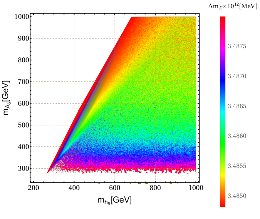
One scalar is the SM like Higgs boson hh with mass of 125 GeV. One another scalar is a new one h5h_{5} with mass takes the values of 150150 GeV 7a; 8a; 9a; 10a; 11a; 12a; 13a or 9696 GeV 96gev1; 96gev2; 96gev3; 96gev4, respectively. The mass value of h5h_{5} depends on some parameters such as λ2,λ3,λϕ\lambda_{2},\lambda_{3},\lambda_{\phi} and the VEVs of the scalar fields in this model. From (92) and (93), we have the correlation between A5,hA_{5},h and h5h_{5} as below:

|mh52−mA52|=𝒪⁡(mh2).\displaystyle|m_{h_{5}}^{2}-m_{A_{5}}^{2}|=\mathcal{O}\left(m_{h}^{2}\right)\,. (94)

From Eq.(94), it follows that in the case vη=vρv_{\eta}=v_{\rho}, the splitting by masses of h5h_{5} and A5A_{5} is about few hundreds GeV.

V Yukawa couplings and top quark FCNC decays

In the quark sector, there are two parts: exotic quarks without mass mixing and ordinary quarks with mass mixing. Because of having no mass mixing, the mass eigenstates of exotic quarks are their original states. Then, we just consider on the mass mixing of ordinary quarks. The mass matrices of ordinary quarks are

Mu=((y6)11​vρvη(y6)12​vρvη(y6)13​vρvη(y6)21​vρvη(y6)22​vρvη(y6)23​vρvη(y3)31(y3)32(y3)33)​vη2=Vu​L​M~u​Vu​R†,M_{u}=\left(\begin{array}[]{ccc}\left(y_{6}\right)_{11}\frac{v_{\rho}}{v_{\eta}}&\left(y_{6}\right)_{12}\frac{v_{\rho}}{v_{\eta}}&\left(y_{6}\right)_{13}\frac{v_{\rho}}{v_{\eta}}\\ \left(y_{6}\right)_{21}\frac{v_{\rho}}{v_{\eta}}&\left(y_{6}\right)_{22}\frac{v_{\rho}}{v_{\eta}}&\left(y_{6}\right)_{23}\frac{v_{\rho}}{v_{\eta}}\\ \left(y_{3}\right)_{31}&\left(y_{3}\right)_{32}&\left(y_{3}\right)_{33}\end{array}\right)\frac{v_{\eta}}{\sqrt{2}}=V_{uL}\widetilde{M}_{u}V_{uR}^{\dagger}\,, (95)

with

M~u=d​i​a​g​(mu,mc,mt)\widetilde{M}_{u}=diag\left(m_{u},m_{c},m_{t}\right)\, (96)

and

Md=((y4)11​vηvρ(y4)12​vηvρ(y4)13​vηvρ(y4)21​vηvρ(y4)22​vηvρ(y4)23​vηvρ(y5)31(y5)32(y5)33)​vρ2=Vd​L​M~d​Vd​R†,M_{d}=\left(\begin{array}[]{ccc}\left(y_{4}\right)_{11}\frac{v_{\eta}}{v_{\rho}}&\left(y_{4}\right)_{12}\frac{v_{\eta}}{v_{\rho}}&\left(y_{4}\right)_{13}\frac{v_{\eta}}{v_{\rho}}\\ \left(y_{4}\right)_{21}\frac{v_{\eta}}{v_{\rho}}&\left(y_{4}\right)_{22}\frac{v_{\eta}}{v_{\rho}}&\left(y_{4}\right)_{23}\frac{v_{\eta}}{v_{\rho}}\\ \left(y_{5}\right)_{31}&\left(y_{5}\right)_{32}&\left(y_{5}\right)_{33}\end{array}\right)\frac{v_{\rho}}{\sqrt{2}}=V_{dL}\widetilde{M}_{d}V_{dR}^{\dagger}\,, (97)

with

M~d=d​i​a​g​(md,ms,mb).\widetilde{M}_{d}=diag\left(m_{d},m_{s},m_{b}\right)\,. (98)
K=Vu​L†​Vd​L.K=V_{uL}^{\dagger}V_{dL}\,. (99)

In these matrices above, all Yukawa couplings of the form (yi)a​b\left(y_{i}\right)_{ab} a,b=1,2,3a,b=1,2,3; i=3,4,5,6i=3,4,5,6 are real and positive. With α=1,2\alpha=1,2 and a=α,3a=\alpha,3, these couplings can be defined by the following equations:

(y6)n​a=2vρ​(Vu​L​M~u​Vu​R†)n​a,(y3)3​a=2vη​(Vu​L​M~u​Vu​R†)3​a\left(y_{6}\right)_{na}=\frac{\sqrt{2}}{v_{\rho}}\left(V_{uL}\widetilde{M}_{u}V_{uR}^{\dagger}\right)_{na},\hskip 28.45274pt\hskip 28.45274pt\left(y_{3}\right)_{3a}=\frac{\sqrt{2}}{v_{\eta}}\left(V_{uL}\widetilde{M}_{u}V_{uR}^{\dagger}\right)_{3a} (100)
(y4)n​a=2vη​(Vd​L​M~d​Vd​R†)n​a,(y5)3​a=2vρ​(Vd​L​M~d​Vd​R†)3​a.\left(y_{4}\right)_{na}=\frac{\sqrt{2}}{v_{\eta}}\left(V_{dL}\widetilde{M}_{d}V_{dR}^{\dagger}\right)_{na},\hskip 28.45274pt\hskip 28.45274pt\left(y_{5}\right)_{3a}=\frac{\sqrt{2}}{v_{\rho}}\left(V_{dL}\widetilde{M}_{d}V_{dR}^{\dagger}\right)_{3a}\,. (101)

From (95) and (97), the diagonalized mass matrix of ordinary quarks are defined as below:

M~u,d=(VL(u,d))†​Mu,d​VR(u,d).\widetilde{M}_{u,d}=\left(V_{L}^{\left(u,d\right)}\right)^{\dagger}M_{u,d}V_{R}^{\left(u,d\right)}\,. (102)

In general, we get:

M~f\displaystyle\widetilde{M}_{f} =\displaystyle= (Mf)d​i​a​g=Vf​L†​Mf​Vf​R,f(L,R)=Vf⁡(L,R)​f~(L,R),\displaystyle\left(M_{f}\right)_{diag}=V_{fL}^{\dagger}M_{f}V_{fR},\hskip 28.45274pt\hskip 28.45274ptf_{\left(L,R\right)}=V_{f\left(L,R\right)}\widetilde{f}_{\left(L,R\right)},
f¯a​L​(Mf)a​b​fb​R\displaystyle\overline{f}_{aL}\left(M_{f}\right)_{ab}f_{bR} =\displaystyle= f~¯k​L​(Vf​L†)k​a​(Mf)a​b​(Vf​R)b​l​f~l​R=f~¯k​L​(Vf​L†​Mf​Vf​R)k​l​f~l​R=f~¯k​L​(M~f)k​l​f~l​R=mfk​f~¯k​L​f~k​R,\displaystyle\overline{\widetilde{f}}_{kL}\left(V_{fL}^{\dagger}\right)_{ka}\left(M_{f}\right)_{ab}\left(V_{fR}\right)_{bl}\widetilde{f}_{lR}=\overline{\widetilde{f}}_{kL}\left(V_{fL}^{\dagger}M_{f}V_{fR}\right)_{kl}\widetilde{f}_{lR}=\overline{\widetilde{f}}_{kL}\left(\widetilde{M}_{f}\right)_{kl}\widetilde{f}_{lR}=m_{f_{k}}\overline{\widetilde{f}}_{kL}\widetilde{f}_{kR},
k\displaystyle k =\displaystyle= 1,2,3.\displaystyle 1,2,3\,. (103)

Here, f~k⁡(L,R)\widetilde{f}_{k\left(L,R\right)} and fk⁡(L,R)f_{k\left(L,R\right)} (k=1,2,3k=1,2,3) are the SM fermionic fields in the mass and interaction bases, respectively. Hence, the SM up and down type quark Yukawa interactions are given by:

−ℒY(u)\displaystyle-\mathcal{L}_{Y}^{\left(u\right)} =\displaystyle= ∑n=12∑a=13(y6)n​a​u¯n​L​vρ+Rρ−i​Iρ2​ua​R+∑a=13(y3)3​a​u¯3​L​vη+Rη1+i​Iη12​ub​R+h.c\displaystyle\sum_{n=1}^{2}\sum_{a=1}^{3}\left(y_{6}\right)_{na}\overline{u}_{nL}\frac{v_{\rho}+R_{\rho}-iI_{\rho}}{\sqrt{2}}u_{aR}+\sum_{a=1}^{3}\left(y_{3}\right)_{3a}\overline{u}_{3L}\frac{v_{\eta}+R_{\eta}^{1}+iI_{\eta}^{1}}{\sqrt{2}}u_{bR}+h.c (104)
=\displaystyle= ∑n=12∑a=13∑b=13∑c=13(y6)n​a​u~¯c​L​((VL(u))†)c​n​vρ+Rρ−i​Iρ2​(VR(u))a​b​u~b​R\displaystyle\sum_{n=1}^{2}\sum_{a=1}^{3}\sum_{b=1}^{3}\sum_{c=1}^{3}\left(y_{6}\right)_{na}\overline{\widetilde{u}}_{cL}\left(\left(V_{L}^{\left(u\right)}\right)^{\dagger}\right)_{cn}\frac{v_{\rho}+R_{\rho}-iI_{\rho}}{\sqrt{2}}\left(V_{R}^{\left(u\right)}\right)_{ab}\widetilde{u}_{bR}
+∑a=13∑b=13∑c=13(y3)3​au~¯c​L((VL(u))†)c​3vη+Rη1+i​Iη12(VR(u))a​bu~b​R+h.c\displaystyle+\sum_{a=1}^{3}\sum_{b=1}^{3}\sum_{c=1}^{3}\left(y_{3}\right)_{3a}\overline{\widetilde{u}}_{cL}\left(\left(V_{L}^{\left(u\right)}\right)^{\dagger}\right)_{c3}\frac{v_{\eta}+R_{\eta}^{1}+iI_{\eta}^{1}}{\sqrt{2}}\left(V_{R}^{\left(u\right)}\right)_{ab}\widetilde{u}_{bR}+h.c
=\displaystyle= ∑n=12∑a=13∑b=13∑c=132vρ​(Vu​L​M~u​Vu​R†)n​a​u~¯c​L​((VL(u))†)c​n​vρ+Rρ−i​Iρ2​(VR(u))a​b​u~b​R\displaystyle\sum_{n=1}^{2}\sum_{a=1}^{3}\sum_{b=1}^{3}\sum_{c=1}^{3}\frac{\sqrt{2}}{v_{\rho}}\left(V_{uL}\widetilde{M}_{u}V_{uR}^{\dagger}\right)_{na}\overline{\widetilde{u}}_{cL}\left(\left(V_{L}^{\left(u\right)}\right)^{\dagger}\right)_{cn}\frac{v_{\rho}+R_{\rho}-iI_{\rho}}{\sqrt{2}}\left(V_{R}^{\left(u\right)}\right)_{ab}\widetilde{u}_{bR}
+∑a=132vη(Vu​LM~uVu​R†)3​au~¯c​L((VL(u))†)c​3vη+Rη1+i​Iη12(VR(u))a​bu~b​R+h.c.\displaystyle+\sum_{a=1}^{3}\frac{\sqrt{2}}{v_{\eta}}\left(V_{uL}\widetilde{M}_{u}V_{uR}^{\dagger}\right)_{3a}\overline{\widetilde{u}}_{cL}\left(\left(V_{L}^{\left(u\right)}\right)^{\dagger}\right)_{c3}\frac{v_{\eta}+R_{\eta}^{1}+iI_{\eta}^{1}}{\sqrt{2}}\left(V_{R}^{\left(u\right)}\right)_{ab}\widetilde{u}_{bR}+h.c\,.
−ℒY(d)\displaystyle-\mathcal{L}_{Y}^{\left(d\right)} =\displaystyle= ∑n=12∑a=13(y4)n​a​d¯n​L​vη+Rη1−i​Iη12​da​R+∑a=13(y5)3​a​d¯3​L​vρ+Rρ+i​Iρ2​db​R+h.c\displaystyle\sum_{n=1}^{2}\sum_{a=1}^{3}\left(y_{4}\right)_{na}\overline{d}_{nL}\frac{v_{\eta}+R_{\eta}^{1}-iI_{\eta}^{1}}{\sqrt{2}}d_{aR}+\sum_{a=1}^{3}\left(y_{5}\right)_{3a}\overline{d}_{3L}\frac{v_{\rho}+R_{\rho}+iI_{\rho}}{\sqrt{2}}d_{bR}+h.c (105)
=\displaystyle= ∑n=12∑a=13∑b=13∑c=13(y4)n​a​d~¯c​L​((VL(d))†)c​n​vη+Rη1−i​Iη12​(VR(d))a​b​d~b​R\displaystyle\sum_{n=1}^{2}\sum_{a=1}^{3}\sum_{b=1}^{3}\sum_{c=1}^{3}\left(y_{4}\right)_{na}\overline{\widetilde{d}}_{cL}\left(\left(V_{L}^{\left(d\right)}\right)^{\dagger}\right)_{cn}\frac{v_{\eta}+R_{\eta}^{1}-iI_{\eta}^{1}}{\sqrt{2}}\left(V_{R}^{\left(d\right)}\right)_{ab}\widetilde{d}_{bR}
+∑a=13∑b=13∑c=13(y5)3​ad~¯c​L((VL(d))†)c​3vρ+Rρ+i​Iρ2(VR(d))a​bd~b​R+h.c\displaystyle+\sum_{a=1}^{3}\sum_{b=1}^{3}\sum_{c=1}^{3}\left(y_{5}\right)_{3a}\overline{\widetilde{d}}_{cL}\left(\left(V_{L}^{\left(d\right)}\right)^{\dagger}\right)_{c3}\frac{v_{\rho}+R_{\rho}+iI_{\rho}}{\sqrt{2}}\left(V_{R}^{\left(d\right)}\right)_{ab}\widetilde{d}_{bR}+h.c
=\displaystyle= ∑n=12∑a=13∑b=13∑c=132vη​(Vd​L​M~d​Vd​R†)n​a​d~¯c​L​((VL(d))†)c​n​vη+Rη1−i​Iη12​(VR(d))a​b​d~b​R\displaystyle\sum_{n=1}^{2}\sum_{a=1}^{3}\sum_{b=1}^{3}\sum_{c=1}^{3}\frac{\sqrt{2}}{v_{\eta}}\left(V_{dL}\widetilde{M}_{d}V_{dR}^{\dagger}\right)_{na}\overline{\widetilde{d}}_{cL}\left(\left(V_{L}^{\left(d\right)}\right)^{\dagger}\right)_{cn}\frac{v_{\eta}+R_{\eta}^{1}-iI_{\eta}^{1}}{\sqrt{2}}\left(V_{R}^{\left(d\right)}\right)_{ab}\widetilde{d}_{bR}
+∑a=13∑b=13∑c=132vρ(Vd​LM~dVd​R†)3​ad~¯c​L((VL(d))†)c​3vρ+Rρ+i​Iρ2(VR(d))a​bd~b​R+h.c.\displaystyle+\sum_{a=1}^{3}\sum_{b=1}^{3}\sum_{c=1}^{3}\frac{\sqrt{2}}{v_{\rho}}\left(V_{dL}\widetilde{M}_{d}V_{dR}^{\dagger}\right)_{3a}\overline{\widetilde{d}}_{cL}\left(\left(V_{L}^{\left(d\right)}\right)^{\dagger}\right)_{c3}\frac{v_{\rho}+R_{\rho}+iI_{\rho}}{\sqrt{2}}\left(V_{R}^{\left(d\right)}\right)_{ab}\widetilde{d}_{bR}+h.c\,.

Replacing Eqs. (50) and (67) in (104) and (105), we found that the Yukawa couplings of hh, h5h_{5} and A5A_{5} with up and down -type SM quarks are given by:

(Γuh)i​j\displaystyle\left(\Gamma_{u}^{h}\right)_{ij} =\displaystyle= cos⁡α2vρ​∑n=12∑a=13((VL(u))†)i​n​(Vu​L​M~u​Vu​R†)n​a​(VR(u))a​j\displaystyle\frac{\cos\alpha_{2}}{v_{\rho}}\sum_{n=1}^{2}\sum_{a=1}^{3}\left(\left(V_{L}^{\left(u\right)}\right)^{\dagger}\right)_{in}\left(V_{uL}\widetilde{M}_{u}V_{uR}^{\dagger}\right)_{na}\left(V_{R}^{\left(u\right)}\right)_{aj} (106)
−sin⁡α2vη∑a=13((VL(u))†)i​3(Vu​LM~uVu​R†)3​a(VR(u))a​j\displaystyle-\frac{\sin\alpha_{2}}{v_{\eta}}\sum_{a=1}^{3}\left(\left(V_{L}^{\left(u\right)}\right)^{\dagger}\right)_{i3}\left(V_{uL}\widetilde{M}_{u}V_{uR}^{\dagger}\right)_{3a}\left(V_{R}^{\left(u\right)}\right)_{aj}
(Γuh5)i​j\displaystyle\left(\Gamma_{u}^{h_{5}}\right)_{ij} =\displaystyle= sin⁡α2vρ​∑n=12∑a=13((VL(u))†)i​n​(Vu​L​M~u​Vu​R†)n​a​(VR(u))a​j\displaystyle\frac{\sin\alpha_{2}}{v_{\rho}}\sum_{n=1}^{2}\sum_{a=1}^{3}\left(\left(V_{L}^{\left(u\right)}\right)^{\dagger}\right)_{in}\left(V_{uL}\widetilde{M}_{u}V_{uR}^{\dagger}\right)_{na}\left(V_{R}^{\left(u\right)}\right)_{aj} (107)
+cos⁡α2vη∑a=13((VL(u))†)i​3(Vu​LM~uVu​R†)3​a(VR(u))a​j\displaystyle+\frac{\cos\alpha_{2}}{v_{\eta}}\sum_{a=1}^{3}\left(\left(V_{L}^{\left(u\right)}\right)^{\dagger}\right)_{i3}\left(V_{uL}\widetilde{M}_{u}V_{uR}^{\dagger}\right)_{3a}\left(V_{R}^{\left(u\right)}\right)_{aj}
(ΓuA5)i​j\displaystyle\left(\Gamma_{u}^{A_{5}}\right)_{ij} =\displaystyle= −isin⁡αvρ∑n=12∑a=13((VL(u))†)i​n(Vu​LM~uVu​R†)n​a(VR(u))a​j\displaystyle-i\frac{\sin\alpha}{v_{\rho}}\sum_{n=1}^{2}\sum_{a=1}^{3}\left(\left(V_{L}^{\left(u\right)}\right)^{\dagger}\right)_{in}\left(V_{uL}\widetilde{M}_{u}V_{uR}^{\dagger}\right)_{na}\left(V_{R}^{\left(u\right)}\right)_{aj} (108)
+icos⁡αvη∑a=13((VL(u))†)i​3(Vu​LM~uVu​R†)3​a(VR(u))a​j\displaystyle+i\frac{\cos\alpha}{v_{\eta}}\sum_{a=1}^{3}\left(\left(V_{L}^{\left(u\right)}\right)^{\dagger}\right)_{i3}\left(V_{uL}\widetilde{M}_{u}V_{uR}^{\dagger}\right)_{3a}\left(V_{R}^{\left(u\right)}\right)_{aj}
(Γdh)i​j\displaystyle\left(\Gamma_{d}^{h}\right)_{ij} =\displaystyle= −sin⁡α2vη∑n=12∑a=13((VL(d))†)i​n(Vd​LM~dVd​R†)n​a(VR(d))a​j\displaystyle-\frac{\sin\alpha_{2}}{v_{\eta}}\sum_{n=1}^{2}\sum_{a=1}^{3}\left(\left(V_{L}^{\left(d\right)}\right)^{\dagger}\right)_{in}\left(V_{dL}\widetilde{M}_{d}V_{dR}^{\dagger}\right)_{na}\left(V_{R}^{\left(d\right)}\right)_{aj} (109)
+cos⁡α2vρ∑a=13((VL(d))†)i​3(Vd​LM~dVd​R†)3​a(VR(d))a​j\displaystyle+\frac{\cos\alpha_{2}}{v_{\rho}}\sum_{a=1}^{3}\left(\left(V_{L}^{\left(d\right)}\right)^{\dagger}\right)_{i3}\left(V_{dL}\widetilde{M}_{d}V_{dR}^{\dagger}\right)_{3a}\left(V_{R}^{\left(d\right)}\right)_{aj}
(Γdh5)i​j\displaystyle\left(\Gamma_{d}^{h_{5}}\right)_{ij} =\displaystyle= cos⁡α2vη​∑n=12∑a=13((VL(d))†)i​n​(Vd​L​M~d​Vd​R†)n​a​(VR(d))a​j\displaystyle\frac{\cos\alpha_{2}}{v_{\eta}}\sum_{n=1}^{2}\sum_{a=1}^{3}\left(\left(V_{L}^{\left(d\right)}\right)^{\dagger}\right)_{in}\left(V_{dL}\widetilde{M}_{d}V_{dR}^{\dagger}\right)_{na}\left(V_{R}^{\left(d\right)}\right)_{aj} (110)
+sin⁡α2vρ∑a=13((VL(d))†)i​3(Vd​LM~dVd​R†)3​a(VR(d))a​j\displaystyle+\frac{\sin\alpha_{2}}{v_{\rho}}\sum_{a=1}^{3}\left(\left(V_{L}^{\left(d\right)}\right)^{\dagger}\right)_{i3}\left(V_{dL}\widetilde{M}_{d}V_{dR}^{\dagger}\right)_{3a}\left(V_{R}^{\left(d\right)}\right)_{aj}
(ΓdA5)i​j\displaystyle\left(\Gamma_{d}^{A_{5}}\right)_{ij} =\displaystyle= −icos⁡αvη∑n=12∑a=13((VL(d))†)i​n(Vd​LM~dVd​R†)n​a(VR(d))a​j\displaystyle-i\frac{\cos\alpha}{v_{\eta}}\sum_{n=1}^{2}\sum_{a=1}^{3}\left(\left(V_{L}^{\left(d\right)}\right)^{\dagger}\right)_{in}\left(V_{dL}\widetilde{M}_{d}V_{dR}^{\dagger}\right)_{na}\left(V_{R}^{\left(d\right)}\right)_{aj} (111)
+isin⁡αvρ∑a=13((VL(d))†)i​3(Vd​LM~dVd​R†)3​a(VR(d))a​j\displaystyle+i\frac{\sin\alpha}{v_{\rho}}\sum_{a=1}^{3}\left(\left(V_{L}^{\left(d\right)}\right)^{\dagger}\right)_{i3}\left(V_{dL}\widetilde{M}_{d}V_{dR}^{\dagger}\right)_{3a}\left(V_{R}^{\left(d\right)}\right)_{aj}

Rewriting the couplings (106) and (109) in another form, one gets:

(Γu,dh)i​j\displaystyle\left(\Gamma_{u,d}^{h}\right)_{ij} =\displaystyle= cos⁡α2vρ​(M~u,d)i​j−cos⁡α2vη​(tan⁡α+tan⁡α2)​(Γh′(u,d))i​j.\displaystyle\frac{\cos\alpha_{2}}{v_{\rho}}\left(\widetilde{M}_{u,d}\right)_{ij}-\frac{\cos\alpha_{2}}{v_{\eta}}(\tan\alpha+\tan\alpha_{2})\left(\Gamma_{h}^{\prime(u,d)}\right)_{ij}\,. (112)

The first term in (112) is a flavor conserving. The second term in (112) is a flavor changing. In order to have flavor conservation for SM-Higgs interactions, the second term should be vanished. Then, one gets the condition below:

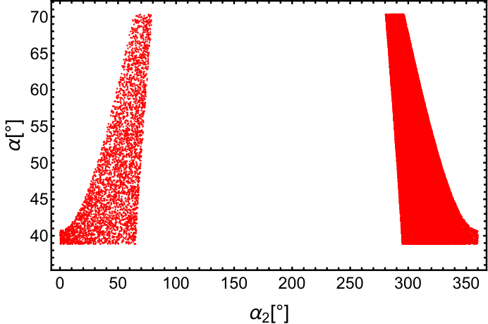
tan⁡α=−tan⁡α2\tan\alpha=-\tan\alpha_{2} (113)

The Eq.(113) gives the condition among vρv_{\rho} and vϕ,vχ,λϕ,λ2,λ3,λ6v_{\phi},v_{\chi},\lambda_{\phi},\lambda_{2},\lambda_{3},\lambda_{6} which guarantees the flavor conservation of SM-Higgs at tree level. In the SM, the resulting top quark FCNCs are strongly suppressed. But in this model, the FCNCs of top quark appear and can be used to look for new physics. The Yukawa couplings of up-type quarks Γu​t,c​th,h5\Gamma_{ut,ct}^{h,h_{5}} allow some decays at tree-level such as: t→h​ut\rightarrow hu or t→h​ct\rightarrow hc. These processes get the branching ratios limited by ATLAS thqATLAS: at 95% C.L. upper limits on the B​r​(t→h​c)=1.1×10⁻³​(8.3×10⁻⁴)Br(t\rightarrow hc)=1.1\times 10^{-3}(8.3\times 10^{-4}) and B​r​(t→h​u)=1.2×10⁻³​(8.3×10⁻⁴)Br(t\rightarrow hu)=1.2\times 10^{-3}(8.3\times 10^{-4}), respectively. The corresponding combined observed (expected) upper limits on the couplings |Γt​ch|=0.064​(0.055)|\Gamma_{tc}^{h}|=0.064(0.055) and |Γt​uh|=0.066​(0.055)|\Gamma_{tu}^{h}|=0.066(0.055), respectively.

Considering the process t→h​ct\rightarrow hc, its branching ratio is given by:

B​r​(t→h​c)=gt​h​c24​π​(mt2−mh2)22​mt​mhΓt,Br(t\rightarrow hc)=\frac{\frac{g_{thc}^{2}}{4\pi}\frac{(m_{t}^{2}-m_{h}^{2})^{2}}{2m_{t}m_{h}}}{\Gamma_{t}}\,, (114)

with Γt=1.32​G​e​V\Gamma_{t}=1.32GeV is the decay width for top quark (mt=172.5​G​e​Vm_{t}=172.5GeV) predicted by SM. And gt​h​cg_{thc} is the coupling defined by ghtc:

gt​h​c2\displaystyle g_{thc}^{2} =\displaystyle= (cos⁡α2vρ​((VL(u))†)23​(Vu​L​M~u​Vu​R†)32​(VR(u))23−sin⁡α2vη​((VL(u))†)23​(Vu​L​M~u​Vu​R†)32​(VR(u))23)2\displaystyle\left(\frac{\cos\alpha_{2}}{v_{\rho}}\left(\left(V_{L}^{\left(u\right)}\right)^{\dagger}\right)_{23}\left(V_{uL}\widetilde{M}_{u}V_{uR}^{\dagger}\right)_{32}\left(V_{R}^{\left(u\right)}\right)_{23}-\frac{\sin\alpha_{2}}{v_{\eta}}\left(\left(V_{L}^{\left(u\right)}\right)^{\dagger}\right)_{23}\left(V_{uL}\widetilde{M}_{u}V_{uR}^{\dagger}\right)_{32}\left(V_{R}^{\left(u\right)}\right)_{23}\right)^{2} (115)
+(cos⁡α2vρ​((VL(u))†)32​(Vu​L​M~u​Vu​R†)23​(VR(u))32−sin⁡α2vη​((VL(u))†)32​(Vu​L​M~u​Vu​R†)23​(VR(u))32)2\displaystyle+\left(\frac{\cos\alpha_{2}}{v_{\rho}}\left(\left(V_{L}^{\left(u\right)}\right)^{\dagger}\right)_{32}\left(V_{uL}\widetilde{M}_{u}V_{uR}^{\dagger}\right)_{23}\left(V_{R}^{\left(u\right)}\right)_{32}-\frac{\sin\alpha_{2}}{v_{\eta}}\left(\left(V_{L}^{\left(u\right)}\right)^{\dagger}\right)_{32}\left(V_{uL}\widetilde{M}_{u}V_{uR}^{\dagger}\right)_{23}\left(V_{R}^{\left(u\right)}\right)_{32}\right)^{2}

We can also get the branching ratio for the process t→h​ut\rightarrow hu as follows:

B​r​(t→h​u)=gt​h​u24​π​(mt2−mh2)22​mt​mhΓt,Br(t\rightarrow hu)=\frac{\frac{g_{thu}^{2}}{4\pi}\frac{(m_{t}^{2}-m_{h}^{2})^{2}}{2m_{t}m_{h}}}{\Gamma_{t}}\,, (116)

with gt​h​ug_{thu} is the coupling that is similarly defined by:

gt​h​u2\displaystyle g_{thu}^{2} =\displaystyle= (cos⁡α2vρ​((VL(u))†)13​(Vu​L​M~u​Vu​R†)31​(VR(u))13−sin⁡α2vη​((VL(u))†)13​(Vu​L​M~u​Vu​R†)31​(VR(u))13)2\displaystyle\left(\frac{\cos\alpha_{2}}{v_{\rho}}\left(\left(V_{L}^{\left(u\right)}\right)^{\dagger}\right)_{13}\left(V_{uL}\widetilde{M}_{u}V_{uR}^{\dagger}\right)_{31}\left(V_{R}^{\left(u\right)}\right)_{13}-\frac{\sin\alpha_{2}}{v_{\eta}}\left(\left(V_{L}^{\left(u\right)}\right)^{\dagger}\right)_{13}\left(V_{uL}\widetilde{M}_{u}V_{uR}^{\dagger}\right)_{31}\left(V_{R}^{\left(u\right)}\right)_{13}\right)^{2} (117)
+(cos⁡α2vρ​((VL(u))†)31​(Vu​L​M~u​Vu​R†)13​(VR(u))31−sin⁡α2vη​((VL(u))†)31​(Vu​L​M~u​Vu​R†)13​(VR(u))31)2\displaystyle+\left(\frac{\cos\alpha_{2}}{v_{\rho}}\left(\left(V_{L}^{\left(u\right)}\right)^{\dagger}\right)_{31}\left(V_{uL}\widetilde{M}_{u}V_{uR}^{\dagger}\right)_{13}\left(V_{R}^{\left(u\right)}\right)_{31}-\frac{\sin\alpha_{2}}{v_{\eta}}\left(\left(V_{L}^{\left(u\right)}\right)^{\dagger}\right)_{31}\left(V_{uL}\widetilde{M}_{u}V_{uR}^{\dagger}\right)_{13}\left(V_{R}^{\left(u\right)}\right)_{31}\right)^{2}

With mh=125m_{h}=125 GeV, mt=172.9m_{t}=172.9 GeV and the branching ratios limited by ATLAS that we mentioned above, we plot the correlation between the mixing angle in range (−π2,−π4)(-\frac{\pi}{2},-\frac{\pi}{4}) and the branching ratios of t→h​qt\rightarrow hq decay with q=u,cq=u,c. Moreover, in this model, we have a light non SM C​PCP even scalar field such as h5h_{5} then the decays t→q​h5t\rightarrow qh_{5} (q=c,uq=c,u) can be under the consideration as well as the decays t→h​qt\rightarrow hq. The couplings of the decays t→q​h5t\rightarrow qh_{5} (q=c,uq=c,u) are defined by:

gt​h5​qi2\displaystyle g_{th_{5}q_{i}}^{2} =\displaystyle= (−sin⁡α2vρ​((VL(u))†)i​3​(Vu​L​M~u​Vu​R†)3​i​(VR(u))i​3−cos⁡α2vη​((VL(u))†)i​3​(Vu​L​M~u​Vu​R†)3​i​(VR(u))i​3)2\displaystyle\left(\frac{-\sin\alpha_{2}}{v_{\rho}}\left(\left(V_{L}^{\left(u\right)}\right)^{\dagger}\right)_{i3}\left(V_{uL}\widetilde{M}_{u}V_{uR}^{\dagger}\right)_{3i}\left(V_{R}^{\left(u\right)}\right)_{i3}-\frac{\cos\alpha_{2}}{v_{\eta}}\left(\left(V_{L}^{\left(u\right)}\right)^{\dagger}\right)_{i3}\left(V_{uL}\widetilde{M}_{u}V_{uR}^{\dagger}\right)_{3i}\left(V_{R}^{\left(u\right)}\right)_{i3}\right)^{2} (118)
+(−sin⁡α2vρ​((VL(u))†)3​i​(Vu​L​M~u​Vu​R†)i​3​(VR(u))3​i−cos⁡α2vη​((VL(u))†)3​i​(Vu​L​M~u​Vu​R†)i​3​(VR(u))3​i)2,\displaystyle+\left(\frac{-\sin\alpha_{2}}{v_{\rho}}\left(\left(V_{L}^{\left(u\right)}\right)^{\dagger}\right)_{3i}\left(V_{uL}\widetilde{M}_{u}V_{uR}^{\dagger}\right)_{i3}\left(V_{R}^{\left(u\right)}\right)_{3i}-\frac{\cos\alpha_{2}}{v_{\eta}}\left(\left(V_{L}^{\left(u\right)}\right)^{\dagger}\right)_{3i}\left(V_{uL}\widetilde{M}_{u}V_{uR}^{\dagger}\right)_{i3}\left(V_{R}^{\left(u\right)}\right)_{3i}\right)^{2}\,,

with q1=u,q2=c,i=1,2q_{1}=u,q_{2}=c,i=1,2. Hence, the branching ratios of t→q​h5t\rightarrow qh_{5} (q=c,uq=c,u) are

B​r​(t→h5​u)=gt​h5​u24​π​(mt2−mh52)22​mt​mh5Γt,B​r​(t→h5​c)=gt​h5​c24​π​(mt2−mh52)22​mt​mh5Γt.\displaystyle Br(t\rightarrow h_{5}u)=\frac{\frac{g_{th_{5}u}^{2}}{4\pi}\frac{(m_{t}^{2}-m_{h_{5}}^{2})^{2}}{2m_{t}m_{h_{5}}}}{\Gamma_{t}}\,,\hskip 8.5359ptBr(t\rightarrow h_{5}c)=\frac{\frac{g_{th_{5}c}^{2}}{4\pi}\frac{(m_{t}^{2}-m_{h_{5}}^{2})^{2}}{2m_{t}m_{h_{5}}}}{\Gamma_{t}}\,. (119)

Considering a benchmark scenario where the h5h_{5} non SM scalar has a mass around 150150 GeV, we have numerically checked that the branching ratios for the t→h5​qt\rightarrow h_{5}q decays (with q=u,cq=u,c) can acquire values of the order of 10−310^{-3}, which are within of the future experimental sensitivities.

In this section, we discuss the implications of the model in meson oscillations, in the h→b¯​bh\rightarrow\bar{b}b, h→l¯​lh\rightarrow\bar{l}l decays as well as in the rare top decays t→c​γt\rightarrow c\gamma and t→u​γt\rightarrow u\gamma. Furthermore, we also determine the couplings of the ALP aa and pseudoscalar A5A_{5} and we provide the corresponding discussion.

V.1 SM like Higgs decays

V.1.1 SM like Higgs decays into two down-type quarks h→b¯​bh\rightarrow\bar{b}b

Using (351), the decay rate of the process h→b¯​bh\rightarrow\bar{b}b is

Γ⁡(h→b¯​b)=∫𝑑Γ=gh​b​b28​π​mh​(1−4​mb2mh2)32\displaystyle\Gamma(h\rightarrow\bar{b}b)=\int d\Gamma=\frac{g_{hbb}^{2}}{8\pi}m_{h}\left(1-\frac{4m_{b}^{2}}{m_{h}^{2}}\right)^{\frac{3}{2}} (120)

with

gh​b​b¯\displaystyle g_{hb\bar{b}} =\displaystyle= cos⁡α2vρ​((VL(d))†)33​(Vd​L​M~d​Vd​R†)33​(VR(d))33−sin⁡α2vη​((VL(d))†)33​(Vd​L​M~d​Vd​R†)33​(VR(d))33\displaystyle\frac{\cos\alpha_{2}}{v_{\rho}}\left(\left(V_{L}^{\left(d\right)}\right)^{\dagger}\right)_{33}\left(V_{dL}\widetilde{M}_{d}V_{dR}^{\dagger}\right)_{33}\left(V_{R}^{\left(d\right)}\right)_{33}-\frac{\sin\alpha_{2}}{v_{\eta}}\left(\left(V_{L}^{\left(d\right)}\right)^{\dagger}\right)_{33}\left(V_{dL}\widetilde{M}_{d}V_{dR}^{\dagger}\right)_{33}\left(V_{R}^{\left(d\right)}\right)_{33} (121)
=\displaystyle= (cos⁡α2vρ−sin⁡α2vη)​mb=(cos⁡α2cos⁡α−sin⁡α2sin⁡α)​mbv=cos⁡α2sin⁡α​(tan⁡α−tan⁡α2)​mbv=2cosα2cos⁡α​mbv\displaystyle\left(\frac{\cos\alpha_{2}}{v_{\rho}}-\frac{\sin\alpha_{2}}{v_{\eta}}\right)m_{b}=\left(\frac{\cos\alpha_{2}}{\cos\alpha}-\frac{\sin\alpha_{2}}{\sin\alpha}\right)\frac{m_{b}}{v}=\frac{\cos\alpha_{2}}{\sin\alpha}(\tan\alpha-\tan\alpha_{2})\frac{m_{b}}{v}=\frac{2\cos\alpha_{2}}{\cos\alpha}\frac{m_{b}}{v}
=\displaystyle= ah​b¯​b​gh​b​b¯S​M.\displaystyle a_{h\bar{b}b}g_{hb\bar{b}}^{SM}.

where ah​b​b¯a_{hb\bar{b}} is the deviation factor from the SM Higgs bottom quark coupling (in the SM this factor is unity). The experimental data constraint on the ah​b¯​ba_{h\bar{b}b} parameter is given by:

ah​b​b¯e​x​p=0.91−0.16+0.17,\displaystyle a_{hb\bar{b}}^{exp}=0.91^{+0.17}_{-0.16}\,, (122)

V.1.2 SM like Higgs decays into two charged leptons h→l¯​lh\rightarrow\bar{l}l

Concerning the lepton sector, the Yukawa interaction for charged leptons are given by:

−ℒY(l)=∑a=13∑b=13ga​b​l¯a​L​vρ+Rρ+i​Iρ2​lb​R+h.c.-\mathcal{L}_{Y}^{\left(l\right)}=\sum_{a=1}^{3}\sum_{b=1}^{3}g_{ab}\overline{l}_{aL}\frac{v_{\rho}+R_{\rho}+iI_{\rho}}{\sqrt{2}}l_{bR}+h.c\,. (123)

Replacing Eq.(50) and Eq.(67) in Eq. (123), we get the Yukawa couplings of hh with leptons as below:

−ℒY(l)\displaystyle-\mathcal{L}_{Y}^{\left(l\right)} ⊃\displaystyle\supset ∑a=13∑b=13ga​bcosα22​l¯a​L​h​lb​R\displaystyle\sum_{a=1}^{3}\sum_{b=1}^{3}\frac{g_{ab}\cos\alpha_{2}}{\sqrt{2}}\overline{l}_{aL}hl_{bR} (124)
⊃\displaystyle\supset ∑a=13(Ml)a​acosα2vρ​l¯a​L​h​la​R\displaystyle\sum_{a=1}^{3}\frac{\left(M_{l}\right)_{aa}\cos\alpha_{2}}{v_{\rho}}\overline{l}_{aL}hl_{aR}
⊃\displaystyle\supset ∑a=13vcosα2vρ​(Ml)a​av​l¯a​L​h​la​R.\displaystyle\sum_{a=1}^{3}\frac{v\cos\alpha_{2}}{v_{\rho}}\frac{\left(M_{l}\right)_{aa}}{v}\overline{l}_{aL}hl_{aR}.
gh​l¯​l=∑a=13vcosα2vρ​(Ml)a​av=ah​l¯​l​gh​l¯​lS​M.g_{h\bar{l}l}=\sum_{a=1}^{3}\frac{v\cos\alpha_{2}}{v_{\rho}}\frac{\left(M_{l}\right)_{aa}}{v}=a_{h\bar{l}l}g_{h\bar{l}l}^{SM}. (125)

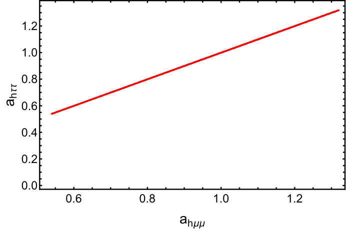
where ah​l¯​la_{h\bar{l}l} is the deviation of the h​l¯​lh\bar{l}l coupling with respect to the SM prediction (in the SM this factor is unity).

Using (351), the decay rate of the process h→μ​μh\rightarrow\mu\mu and h→τ​τh\rightarrow\tau\tau are

Γ⁡(h→μ​μ)=∫𝑑Γ=g(h,μ,μ)28​π​mh​(1−4​mμ2mh2)32=(vcosα2vρ)2​mμ2v2​mh8​π​(1−4​mμ2mh2)32=(cos⁡α2cos⁡α)2​mμ2v2​mh8​π​(1−4​mμ2mh2)32\displaystyle\Gamma(h\rightarrow\mu\mu)=\int d\Gamma=\frac{g_{(h,\mu,\mu)}^{2}}{8\pi}m_{h}\left(1-\frac{4m_{\mu}^{2}}{m_{h}^{2}}\right)^{\frac{3}{2}}=\left(\frac{v\cos\alpha_{2}}{v_{\rho}}\right)^{2}\frac{m_{\mu}^{2}}{v^{2}}\frac{m_{h}}{8\pi}\left(1-\frac{4m_{\mu}^{2}}{m_{h}^{2}}\right)^{\frac{3}{2}}=\left(\frac{\cos\alpha_{2}}{\cos\alpha}\right)^{2}\frac{m_{\mu}^{2}}{v^{2}}\frac{m_{h}}{8\pi}\left(1-\frac{4m_{\mu}^{2}}{m_{h}^{2}}\right)^{\frac{3}{2}} (126)
Γ⁡(h→τ​τ)=∫𝑑Γ=g(h,τ,τ)28​π​mh​(1−4​mτ2mh2)32=(vcosα2vρ)2​mτ2v2​mh8​π​(1−4​mτ2mh2)32=(cos⁡α2cos⁡α)2​mτ2v2​mh8​π​(1−4​mτ2mh2)32\displaystyle\Gamma(h\rightarrow\tau\tau)=\int d\Gamma=\frac{g_{(h,\tau,\tau)}^{2}}{8\pi}m_{h}\left(1-\frac{4m_{\tau}^{2}}{m_{h}^{2}}\right)^{\frac{3}{2}}=\left(\frac{v\cos\alpha_{2}}{v_{\rho}}\right)^{2}\frac{m_{\tau}^{2}}{v^{2}}\frac{m_{h}}{8\pi}\left(1-\frac{4m_{\tau}^{2}}{m_{h}^{2}}\right)^{\frac{3}{2}}=\left(\frac{\cos\alpha_{2}}{\cos\alpha}\right)^{2}\frac{m_{\tau}^{2}}{v^{2}}\frac{m_{h}}{8\pi}\left(1-\frac{4m_{\tau}^{2}}{m_{h}^{2}}\right)^{\frac{3}{2}} (127)

From (126) and (127), one can get the constraints of the mixing angle α2\alpha_{2} in this model. Using the following experimental allowed values of the parameters higgsll:

ah​μ​μe​x​p=0.72−0.72+0.50,ah​τ​τe​x​p=0.93−0.13+0.13,\displaystyle a_{h\mu\mu}^{exp}=0.72^{+0.50}_{-0.72}\,,\hskip 56.9055pta_{h\tau\tau}^{exp}=0.93^{+0.13}_{-0.13}\,, (128)

we can obtain plots where the allowed range of the mixing angle in the C​PCP even scalar sector is shown. Furthermore, we have found the our obtained values for the ah​μ​μ,τ​τa_{h\mu\mu,\tau\tau} parameters range from about 0.60.6 up to about 1.21.2, which is consistent with their current experimental bounds. This is shown in figure 1, which displays a linear correlation between the ah​τ​τa_{h\tau\tau} and ah​μ​μa_{h\mu\mu} parameters.

Refer to caption
Figure 1: Correlation between the ah​τ​τa_{h\tau\tau} and ah​μ​μa_{h\mu\mu} parameters.

Requiring the consistency of the rates for the h→μ¯​μh\rightarrow\bar{\mu}\mu, h→τ¯​τh\rightarrow\bar{\tau}\tau and h→b¯​bh\rightarrow\bar{b}b decays with their corresponding experimentally allowed ranges, we display in figure 2 the correlation between the mixing angles α\alpha and α2\alpha_{2}.

Refer to caption
Figure 2: Correlation between the mixing angles α\alpha and α2\alpha_{2} consistent with the experimental values of the h→μ¯​μh\rightarrow\bar{\mu}\mu, h→τ¯​τh\rightarrow\bar{\tau}\tau and h→b¯​bh\rightarrow\bar{b}b decay rates.

From the Fig.(2), with α\alpha in range 38o38^{o} ≤α≤70o\leq\alpha\leq 70^{o} , we get the following constraints for the mixing angle α2\alpha_{2}:

0o≤α2≤75o,or280o≤α2≤360o.0^{o}\,\leq\alpha_{2}\leq 75^{o}\,,\hskip 8.5359pt\mbox{or}\,\hskip 8.5359pt280^{o}\,\leq\alpha_{2}\leq 360^{o}\ \,. (129)

We will use this constraint to analyze the meson oscillations of this model in the subsection below.

V.2 Meson oscillations

In this section, we analyze the consequences of the model under consideration in the K0−K¯0K^{0}-\bar{K}^{0}, Bd0−B¯d0B_{d}^{0}-\bar{B}_{d}^{0} and Bs0−B¯s0B_{s}^{0}-\bar{B}_{s}^{0} meson oscillations. These meson oscillations are caused by flavor violating scalar and Z′Z^{\prime} interactions in the down type quark sector. The K0−K¯0K^{0}-\bar{K}^{0}, Bd0−B¯d0B_{d}^{0}-\bar{B}_{d}^{0} and Bs0−B¯s0B_{s}^{0}-\bar{B}_{s}^{0} meson mixings are described by the following effective Hamiltonians:

ℋe​f​f(K0−K¯0)=GF2​mW216​π2​∑i=13Ci(K0−K¯0)​(μ)​Oi(K0−K¯0)​(μ)+4​2​GF​cW4​mZ2(3−4​sW2)​mZ′2​|(VD​L∗)32​(VD​L)31|2​O4(K0−K¯0),\mathcal{H}_{eff}^{\left(K^{0}-\bar{K}^{0}\right)}\mathcal{=}\frac{G_{F}^{2}m_{W}^{2}}{16\pi^{2}}\sum_{i=1}^{3}C_{i}^{\left(K^{0}-\bar{K}^{0}\right)}\left(\mu\right)O_{i}^{\left(K^{0}-\bar{K}^{0}\right)}\left(\mu\right)+\frac{4\sqrt{2}G_{F}c_{W}^{4}m_{Z}^{2}}{\left(3-4s_{W}^{2}\right)m_{Z^{\prime}}^{2}}\left|\left(V_{DL}^{\ast}\right)_{32}\left(V_{DL}\right)_{31}\right|^{2}O_{4}^{\left(K^{0}-\bar{K}^{0}\right)}, (130)
ℋe​f​f(Bd0−B¯d0)=GF2​mW216​π2​∑i=13Ci(Bd0−B¯d0)​(μ)​Oi(Bd0−B¯d0)​(μ)+4​2​GF​cW4​mZ2(3−4​sW2)​mZ′2​|(VD​L∗)31​(VD​L)33|2​O4(Bd0−B¯d0),\mathcal{H}_{eff}^{\left(B_{d}^{0}-\bar{B}_{d}^{0}\right)}\mathcal{=}\frac{G_{F}^{2}m_{W}^{2}}{16\pi^{2}}\sum_{i=1}^{3}C_{i}^{\left(B_{d}^{0}-\bar{B}_{d}^{0}\right)}\left(\mu\right)O_{i}^{\left(B_{d}^{0}-\bar{B}_{d}^{0}\right)}\left(\mu\right)+\frac{4\sqrt{2}G_{F}c_{W}^{4}m_{Z}^{2}}{\left(3-4s_{W}^{2}\right)m_{Z^{\prime}}^{2}}\left|\left(V_{DL}^{\ast}\right)_{31}\left(V_{DL}\right)_{33}\right|^{2}O_{4}^{\left(B_{d}^{0}-\bar{B}_{d}^{0}\right)}, (131)
ℋe​f​f(Bs0−B¯s0)=GF2​mW216​π2​∑i=13Ci(Bs0−B¯s0)​(μ)​Oi(Bs0−B¯s0)​(μ)+4​2​GF​cW4​mZ2(3−4​sW2)​mZ′2​|(VD​L∗)32​(VD​L)33|2​O4(Bs0−B¯s0),\mathcal{H}_{eff}^{\left(B_{s}^{0}-\bar{B}_{s}^{0}\right)}\mathcal{=}\frac{G_{F}^{2}m_{W}^{2}}{16\pi^{2}}\sum_{i=1}^{3}C_{i}^{\left(B_{s}^{0}-\bar{B}_{s}^{0}\right)}\left(\mu\right)O_{i}^{\left(B_{s}^{0}-\bar{B}_{s}^{0}\right)}\left(\mu\right)+\frac{4\sqrt{2}G_{F}c_{W}^{4}m_{Z}^{2}}{\left(3-4s_{W}^{2}\right)m_{Z^{\prime}}^{2}}\left|\left(V_{DL}^{\ast}\right)_{32}\left(V_{DL}\right)_{33}\right|^{2}O_{4}^{\left(B_{s}^{0}-\bar{B}_{s}^{0}\right)}, (132)

where VD​LV_{DL} is the rotation matrix that diagonalizes MD​MD†M_{D}M_{D}^{\dagger} according to VD​L†​MD​MD†​VD​L=d​i​a​g​(md2,ms2,mb2)V_{DL}^{\dagger}M_{D}M_{D}^{\dagger}V_{DL}=diag(m^{2}_{d},m^{2}_{s},m^{2}_{b}) being MDM_{D} the SM down type quark mass matrix. Furthermore, the operators appearing in Eqs. (130), (131) and (132) are given by:

O1(K0−K¯0)\displaystyle O_{1}^{\left(K^{0}-\bar{K}^{0}\right)} =\displaystyle= (s¯​PL​d)​(s¯​PL​d),O2(K0−K¯0)=(s¯​PR​d)​(s¯​PR​d),\displaystyle\left(\overline{s}P_{L}d\right)\left(\overline{s}P_{L}d\right),\hskip 19.91684pt\hskip 19.91684ptO_{2}^{\left(K^{0}-\bar{K}^{0}\right)}=\left(\overline{s}P_{R}d\right)\left(\overline{s}P_{R}d\right),\hskip 19.91684pt (133)
O3(K0−K¯0)\displaystyle O_{3}^{\left(K^{0}-\bar{K}^{0}\right)} =\displaystyle= (s¯​PL​d)​(s¯​PR​d),O4(K0−K¯0)=(s¯​γμ​PL​d)​(s¯​γμ​PL​d),\displaystyle\left(\overline{s}P_{L}d\right)\left(\overline{s}P_{R}d\right),\hskip 19.91684pt\hskip 19.91684ptO_{4}^{\left(K^{0}-\bar{K}^{0}\right)}=\left(\overline{s}\gamma_{\mu}P_{L}d\right)\left(\overline{s}\gamma^{\mu}P_{L}d\right), (134)
O1(Bd0−B¯d0)\displaystyle O_{1}^{\left(B_{d}^{0}-\bar{B}_{d}^{0}\right)} =\displaystyle= (d¯​PL​b)​(d¯​PL​b),O2(Bd0−B¯d0)=(d¯​PR​b)​(d¯​PR​b),\displaystyle\left(\overline{d}P_{L}b\right)\left(\overline{d}P_{L}b\right),\hskip 19.91684pt\hskip 19.91684ptO_{2}^{\left(B_{d}^{0}-\bar{B}_{d}^{0}\right)}=\left(\overline{d}P_{R}b\right)\left(\overline{d}P_{R}b\right),\hskip 19.91684pt (135)
O3(Bd0−B¯d0)\displaystyle O_{3}^{\left(B_{d}^{0}-\bar{B}_{d}^{0}\right)} =\displaystyle= (d¯​PL​b)​(d¯​PR​b),O4(Bd0−B¯d0)=(d¯​γμ​PL​b)​(d¯​γμ​PL​b),\displaystyle\left(\overline{d}P_{L}b\right)\left(\overline{d}P_{R}b\right),\hskip 19.91684pt\hskip 19.91684ptO_{4}^{\left(B_{d}^{0}-\bar{B}_{d}^{0}\right)}=\left(\overline{d}\gamma_{\mu}P_{L}b\right)\left(\overline{d}\gamma^{\mu}P_{L}b\right), (136)
O1(Bs0−B¯s0)\displaystyle O_{1}^{\left(B_{s}^{0}-\bar{B}_{s}^{0}\right)} =\displaystyle= (s¯​PL​b)​(s¯​PL​b),O2(Bs0−B¯s0)=(s¯​PR​b)​(s¯​PR​b),\displaystyle\left(\overline{s}P_{L}b\right)\left(\overline{s}P_{L}b\right),\hskip 19.91684pt\hskip 19.91684ptO_{2}^{\left(B_{s}^{0}-\bar{B}_{s}^{0}\right)}=\left(\overline{s}P_{R}b\right)\left(\overline{s}P_{R}b\right), (137)
O3(Bs0−B¯s0)\displaystyle O_{3}^{\left(B_{s}^{0}-\bar{B}_{s}^{0}\right)} =\displaystyle= (s¯​PL​b)​(s¯​PL​b),O4(Bs0−B¯s0)=(s¯​γμ​PL​b)​(s¯​γμ​PL​b),\displaystyle\left(\overline{s}P_{L}b\right)\left(\overline{s}P_{L}b\right),\hskip 19.91684pt\hskip 19.91684ptO_{4}^{\left(B_{s}^{0}-\bar{B}_{s}^{0}\right)}=\left(\overline{s}\gamma_{\mu}P_{L}b\right)\left(\overline{s}\gamma^{\mu}P_{L}b\right), (138)

and the Wilson coefficients read:

C1(K0−K¯0)\displaystyle C_{1}^{\left(K^{0}-\bar{K}^{0}\right)} =\displaystyle= 16​π2GF2​mW2​(gh​s¯R​dL2mh2+gh5​s¯R​dL2mh52−gA5​s¯R​dL2mA52),\displaystyle\frac{16\pi^{2}}{G_{F}^{2}m_{W}^{2}}\left(\frac{g_{h\overline{s}_{R}d_{L}}^{2}}{m_{h}^{2}}+\frac{g_{h_{5}\overline{s}_{R}d_{L}}^{2}}{m_{h_{5}}^{2}}-\frac{g_{A_{5}\overline{s}_{R}d_{L}}^{2}}{m_{A_{5}}^{2}}\right), (139)
C2(K0−K¯0)\displaystyle C_{2}^{\left(K^{0}-\bar{K}^{0}\right)} =\displaystyle= 16​π2GF2​mW2​(gh​s¯L​dR2mh2+gh5​s¯L​dR2mh52−gA5​s¯L​dR2mA52),\displaystyle\frac{16\pi^{2}}{G_{F}^{2}m_{W}^{2}}\left(\frac{g_{h\overline{s}_{L}d_{R}}^{2}}{m_{h}^{2}}+\frac{g_{h_{5}\overline{s}_{L}d_{R}}^{2}}{m_{h_{5}}^{2}}-\frac{g_{A_{5}\overline{s}_{L}d_{R}}^{2}}{m_{A_{5}}^{2}}\right), (140)
C3(K0−K¯0)\displaystyle C_{3}^{\left(K^{0}-\bar{K}^{0}\right)} =\displaystyle= 16​π2GF2​mW2​(gh​s¯R​dL​gh​s¯L​dRmh2+gh5​s¯R​dL​gh5​s¯L​dRmh52−gA5​s¯R​dL​gA5​s¯L​dRmA52),\displaystyle\frac{16\pi^{2}}{G_{F}^{2}m_{W}^{2}}\left(\frac{g_{h\overline{s}_{R}d_{L}}g_{h\overline{s}_{L}d_{R}}}{m_{h}^{2}}+\frac{g_{h_{5}\overline{s}_{R}d_{L}}g_{h_{5}\overline{s}_{L}d_{R}}}{m_{h_{5}}^{2}}-\frac{g_{A_{5}\overline{s}_{R}d_{L}}g_{A_{5}\overline{s}_{L}d_{R}}}{m_{A_{5}}^{2}}\right), (141)
C1(Bd0−B¯d0)\displaystyle C_{1}^{\left(B_{d}^{0}-\bar{B}_{d}^{0}\right)} =\displaystyle= 16​π2GF2​mW2​(gh​d¯R​bL2mh2+gh5​d¯R​bL2mh52−gA5​d¯R​bL2mA52),\displaystyle\frac{16\pi^{2}}{G_{F}^{2}m_{W}^{2}}\left(\frac{g_{h\overline{d}_{R}b_{L}}^{2}}{m_{h}^{2}}+\frac{g_{h_{5}\overline{d}_{R}b_{L}}^{2}}{m_{h_{5}}^{2}}-\frac{g_{A_{5}\overline{d}_{R}b_{L}}^{2}}{m_{A_{5}}^{2}}\right), (142)
C2(Bd0−B¯d0)\displaystyle C_{2}^{\left(B_{d}^{0}-\bar{B}_{d}^{0}\right)} =\displaystyle= 16​π2GF2​mW2​(gh​d¯L​bR2mh2+gh5​d¯L​bR2mh52−gA5​d¯L​bR2mA52),\displaystyle\frac{16\pi^{2}}{G_{F}^{2}m_{W}^{2}}\left(\frac{g_{h\overline{d}_{L}b_{R}}^{2}}{m_{h}^{2}}+\frac{g_{h_{5}\overline{d}_{L}b_{R}}^{2}}{m_{h_{5}}^{2}}-\frac{g_{A_{5}\overline{d}_{L}b_{R}}^{2}}{m_{A_{5}}^{2}}\right), (143)
C3(Bd0−B¯d0)\displaystyle C_{3}^{\left(B_{d}^{0}-\bar{B}_{d}^{0}\right)} =\displaystyle= 16​π2GF2​mW2​(gh​d¯R​bL​gh​d¯L​bRmh2+gh5​d¯R​bL​gh5​d¯L​bRmh52−gA5​d¯R​bL​gA5​d¯L​bRmA52),\displaystyle\frac{16\pi^{2}}{G_{F}^{2}m_{W}^{2}}\left(\frac{g_{h\overline{d}_{R}b_{L}}g_{h\overline{d}_{L}b_{R}}}{m_{h}^{2}}+\frac{g_{h_{5}\overline{d}_{R}b_{L}}g_{h_{5}\overline{d}_{L}b_{R}}}{m_{h_{5}}^{2}}-\frac{g_{A_{5}\overline{d}_{R}b_{L}}g_{A_{5}\overline{d}_{L}b_{R}}}{m_{A_{5}}^{2}}\right), (144)
C1(Bs0−B¯s0)\displaystyle C_{1}^{\left(B_{s}^{0}-\bar{B}_{s}^{0}\right)} =\displaystyle= 16​π2GF2​mW2​(gh​s¯R​bL2mh2+gh5​s¯R​bL2mh52−gA5​s¯R​bL2mA52),\displaystyle\frac{16\pi^{2}}{G_{F}^{2}m_{W}^{2}}\left(\frac{g_{h\overline{s}_{R}b_{L}}^{2}}{m_{h}^{2}}+\frac{g_{h_{5}\overline{s}_{R}b_{L}}^{2}}{m_{h_{5}}^{2}}-\frac{g_{A_{5}\overline{s}_{R}b_{L}}^{2}}{m_{A_{5}}^{2}}\right), (145)
C2(Bs0−B¯s0)\displaystyle C_{2}^{\left(B_{s}^{0}-\bar{B}_{s}^{0}\right)} =\displaystyle= 16​π2GF2​mW2​(gh​s¯L​bR2mh2+gh5​s¯L​bR2mh52−gA5​s¯L​bR2mA52),\displaystyle\frac{16\pi^{2}}{G_{F}^{2}m_{W}^{2}}\left(\frac{g_{h\overline{s}_{L}b_{R}}^{2}}{m_{h}^{2}}+\frac{g_{h_{5}\overline{s}_{L}b_{R}}^{2}}{m_{h_{5}}^{2}}-\frac{g_{A_{5}\overline{s}_{L}b_{R}}^{2}}{m_{A_{5}}^{2}}\right), (146)
C3(Bs0−B¯s0)\displaystyle C_{3}^{\left(B_{s}^{0}-\bar{B}_{s}^{0}\right)} =\displaystyle= 16​π2GF2​mW2​(gh​s¯R​bL​gh​s¯L​bRmh2+gh5​s¯R​bL​gh5​s¯L​bRmh52−gA5​s¯R​bL​gA5​s¯L​bRmA52),\displaystyle\frac{16\pi^{2}}{G_{F}^{2}m_{W}^{2}}\left(\frac{g_{h\overline{s}_{R}b_{L}}g_{h\overline{s}_{L}b_{R}}}{m_{h}^{2}}+\frac{g_{h_{5}\overline{s}_{R}b_{L}}g_{h_{5}\overline{s}_{L}b_{R}}}{m_{h_{5}}^{2}}-\frac{g_{A_{5}\overline{s}_{R}b_{L}}g_{A_{5}\overline{s}_{L}b_{R}}}{m_{A_{5}}^{2}}\right), (147)

with ga​b​cg_{abc} are the couplings between the scalar a=h,h5,A5a=h,h_{5},A_{5} and down-type quarks b=d¯L,Rib=\bar{d}_{L,R}^{i}, c=dL,Rjc=d_{L,R}^{j}, i,j=1,2,3i,j=1,2,3, i≠ji\neq j.
On the other hand, the K−K¯K-\bar{K}, Bd0−B¯d0B_{d}^{0}-\bar{B}_{d}^{0} and Bs0−B¯s0B_{s}^{0}-\bar{B}_{s}^{0} mass splittings are given by:

Δ​mK=(Δ​mK)S​M+Δ​mK(N​P),Δ​mBd=(Δ​mBd)S​M+Δ​mBd(N​P),Δ​mBs=(Δ​mBs)S​M+Δ​mBs(N​P),\Delta m_{K}=\left(\Delta m_{K}\right)_{SM}+\Delta m_{K}^{\left(NP\right)},\hskip 8.5359pt\Delta m_{B_{d}}=\left(\Delta m_{B_{d}}\right)_{SM}+\Delta m_{B_{d}}^{\left(NP\right)},\hskip 8.5359pt\Delta m_{B_{s}}=\left(\Delta m_{B_{s}}\right)_{SM}+\Delta m_{B_{s}}^{\left(NP\right)}, (148)

where (Δ​mK)S​M\left(\Delta m_{K}\right)_{SM}, (Δ​mBd)S​M\left(\Delta m_{B_{d}}\right)_{SM} and (Δ​mBs)S​M\left(\Delta m_{B_{s}}\right)_{SM} are the SM contributions, whereas Δ​mK(N​P)\Delta m_{K}^{\left(NP\right)} , Δ​mBd(N​P)\Delta m_{B_{d}}^{\left(NP\right)} and (Δ​mBs)S​M\left(\Delta m_{B_{s}}\right)_{SM} are new physics contributions.
In the model under consideration, the new physics contributions to the meson differences are given by:

Δ​mK(N​P)\displaystyle\Delta m_{K}^{\left(NP\right)} =\displaystyle= 4​2​GF​cW4​mZ2(3−4​sW2)​mZ′2​|(VD​L∗)32​(VD​L)31|2​fK2​BK​ηK​mK\displaystyle\frac{4\sqrt{2}G_{F}c_{W}^{4}m_{Z}^{2}}{\left(3-4s_{W}^{2}\right)m_{Z^{\prime}}^{2}}\left|\left(V_{DL}^{\ast}\right)_{32}\left(V_{DL}\right)_{31}\right|^{2}f_{K}^{2}B_{K}\eta_{K}m_{K}
+GF2​mW26​π2​mK​fK2​ηK​BK​[P2(K0−K¯0)​C3(K0−K¯0)+P1(K0−K¯0)​(C1(K0−K¯0)+C2(K0−K¯0))],\displaystyle+\frac{G_{F}^{2}m_{W}^{2}}{6\pi^{2}}m_{K}f_{K}^{2}\eta_{K}B_{K}\left[P_{2}^{\left(K^{0}-\bar{K}^{0}\right)}C_{3}^{\left(K^{0}-\bar{K}^{0}\right)}+P_{1}^{\left(K^{0}-\bar{K}^{0}\right)}\left(C_{1}^{\left(K^{0}-\bar{K}^{0}\right)}+C_{2}^{\left(K^{0}-\bar{K}^{0}\right)}\right)\right]\,,
Δ​mBd(N​P)\displaystyle\Delta m_{B_{d}}^{\left(NP\right)} =\displaystyle= 4​2​GF​cW4​mZ2(3−4​sW2)​mZ′2​|(VD​L∗)31​(VD​L)33|2​fBd2​BBd​ηBd​mBd\displaystyle\frac{4\sqrt{2}G_{F}c_{W}^{4}m_{Z}^{2}}{\left(3-4s_{W}^{2}\right)m_{Z^{\prime}}^{2}}\left|\left(V_{DL}^{\ast}\right)_{31}\left(V_{DL}\right)_{33}\right|^{2}f_{B_{d}}^{2}B_{B_{d}}\eta_{B_{d}}m_{B_{d}}
+GF2​mW26​π2​mBd​fBd2​ηBd​BBd​[P2(Bd0−B¯d0)​C3(Bd0−B¯d0)+P1(Bd0−B¯d0)​(C1(Bd0−B¯d0)+C2(Bd0−B¯d0))],\displaystyle+\frac{G_{F}^{2}m_{W}^{2}}{6\pi^{2}}m_{B_{d}}f_{B_{d}}^{2}\eta_{B_{d}}B_{B_{d}}\left[P_{2}^{\left(B_{d}^{0}-\bar{B}_{d}^{0}\right)}C_{3}^{\left(B_{d}^{0}-\bar{B}_{d}^{0}\right)}+P_{1}^{\left(B_{d}^{0}-\bar{B}_{d}^{0}\right)}\left(C_{1}^{\left(B_{d}^{0}-\bar{B}_{d}^{0}\right)}+C_{2}^{\left(B_{d}^{0}-\bar{B}_{d}^{0}\right)}\right)\right]\,,
Δ​mBs(N​P)\displaystyle\Delta m_{B_{s}}^{\left(NP\right)} =\displaystyle= 4​2​GF​cW4​mZ2(3−4​sW2)​mZ′2​|(VD​L∗)32​(VD​L)33|2​fBs2​BBs​ηBs​mBs\displaystyle\frac{4\sqrt{2}G_{F}c_{W}^{4}m_{Z}^{2}}{\left(3-4s_{W}^{2}\right)m_{Z^{\prime}}^{2}}\left|\left(V_{DL}^{\ast}\right)_{32}\left(V_{DL}\right)_{33}\right|^{2}f_{B_{s}}^{2}B_{B_{s}}\eta_{B_{s}}m_{B_{s}}
+GF2​mW26​π2​mBs​fBs2​ηBs​BBs​[P2(Bs0−B¯s0)​C3(Bs0−B¯s0)+P1(Bs0−B¯s0)​(C1(Bs0−B¯s0)+C2(Bs0−B¯s0))]\displaystyle+\frac{G_{F}^{2}m_{W}^{2}}{6\pi^{2}}m_{B_{s}}f_{B_{s}}^{2}\eta_{B_{s}}B_{B_{s}}\left[P_{2}^{\left(B_{s}^{0}-\bar{B}_{s}^{0}\right)}C_{3}^{\left(B_{s}^{0}-\bar{B}_{s}^{0}\right)}+P_{1}^{\left(B_{s}^{0}-\bar{B}_{s}^{0}\right)}\left(C_{1}^{\left(B_{s}^{0}-\bar{B}_{s}^{0}\right)}+C_{2}^{\left(B_{s}^{0}-\bar{B}_{s}^{0}\right)}\right)\right]

Using the following parameters Zyla:2020zbs:

(Δ​mK)exp\displaystyle\left(\Delta m_{K}\right)_{\exp} =\displaystyle= (3.484±0.006)×10−12​MeV,(Δ​mK)SM=3.483×10⁻¹²​MeV\displaystyle\left(3.484\pm 0.006\right)\times 10^{-12}\,\rm{MeV},\hskip 42.67912pt\left(\Delta m_{K}\right)_{SM}=3.483\times 10^{-12}\,\rm{MeV}
fK\displaystyle f_{K} =\displaystyle= 155.7​MeV,BK=0.85,ηK=0.57,\displaystyle 155.7\,\rm{MeV},\hskip 42.67912ptB_{K}=0.85,\hskip 42.67912pt\eta_{K}=0.57,
P1(K0−K¯0)\displaystyle P_{1}^{\left(K^{0}-\bar{K}^{0}\right)} =\displaystyle= −9.3,P2(K0−K¯0)=30.6,mK=(497.611±0.013)​MeV,\displaystyle-9.3,\hskip 42.67912ptP_{2}^{\left(K^{0}-\bar{K}^{0}\right)}=30.6,\hskip 42.67912ptm_{K}=\left(497.611\pm 0.013\right)\,\rm{MeV},\hskip 42.67912pt (149)
(Δ​mBd)exp\displaystyle\left(\Delta m_{B_{d}}\right)_{\exp} =\displaystyle= (3.334±0.013)×10−10​MeV,(Δ​mBd)SM=(3.653±0.037±0.019)×10−10​MeV,\displaystyle\left(3.334\pm 0.013\right)\times 10^{-10}\,\rm{MeV},\hskip 42.67912pt\left(\Delta m_{B_{d}}\right)_{SM}=\left(3.653\pm 0.037\pm 0.019\right)\times 10^{-10}\,\rm{MeV},
fBd\displaystyle f_{B_{d}} =\displaystyle= 188​MeV,BBd=1.26,ηBd=0.55,\displaystyle 188\,\rm{MeV},\hskip 42.67912ptB_{B_{d}}=1.26,\hskip 42.67912pt\eta_{B_{d}}=0.55,
P1(Bd0−B¯d0)\displaystyle P_{1}^{\left(B_{d}^{0}-\bar{B}_{d}^{0}\right)} =\displaystyle= −0.52,P2(Bd0−B¯d0)=0.88,mBd=(5279.65±0.12)​MeV,\displaystyle-0.52,\hskip 42.67912ptP_{2}^{\left(B_{d}^{0}-\bar{B}_{d}^{0}\right)}=0.88,\hskip 42.67912ptm_{B_{d}}=\left(5279.65\pm 0.12\right)\,\rm{MeV},\hskip 42.67912pt (150)
(Δ​mBs)exp\displaystyle\left(\Delta m_{B_{s}}\right)_{\exp} =\displaystyle= (1.1683±0.0013)×10−8​MeV,(Δ​mBs)SM=(1.1577±0.022±0.051)×10−8​MeV,\displaystyle\left(1.1683\pm 0.0013\right)\times 10^{-8}\,\rm{MeV},\hskip 42.67912pt\left(\Delta m_{B_{s}}\right)_{SM}=\left(1.1577\pm 0.022\pm 0.051\right)\times 10^{-8}\,\rm{MeV},
fBs\displaystyle f_{B_{s}} =\displaystyle= 225​MeV,BBs=1.33,ηBs=0.55,\displaystyle 225\,\rm{MeV},\hskip 42.67912ptB_{B_{s}}=1.33,\hskip 42.67912pt\eta_{B_{s}}=0.55,
P1(Bs0−B¯s0)\displaystyle P_{1}^{\left(B_{s}^{0}-\bar{B}_{s}^{0}\right)} =\displaystyle= −0.52,P2(Bs0−B¯s0)=0.88,mBs=(5366.9±0.12)​MeV,\displaystyle-0.52,\hskip 42.67912ptP_{2}^{\left(B_{s}^{0}-\bar{B}_{s}^{0}\right)}=0.88,\hskip 42.67912ptm_{B_{s}}=\left(5366.9\pm 0.12\right)\,\rm{MeV},\hskip 42.67912pt (151)
Refer to caption
Figure 3: Correlation of the Δ​mK\Delta m_{K} meson mass splitting with the heayy C​PCP even scalar mass mh5m_{h^{5}}.
Refer to caption
Figure 4: Correlation between Δ​mBd\Delta m_{B_{d}} and Δ​mBs\Delta m_{B_{s}} meson mass splittings.
Refer to caption
Figure 5: Allowed region in the mA5−mh5m_{A_{5}}-m_{h_{5}} plane consistent with the constraints on Δ​mK\Delta m_{K}, Δ​mBd\Delta m_{B_{d}} and Δ​mBs\Delta m_{B_{s}} meson mass splittings.

We plot in Fig. 3 the correlation between of the Δ​mK\Delta m_{K} meson mass splitting with the non SM C​PCP even scalar mass mh5m_{h_{5}}, whereas in Fig. (5) we display the allowed region in the mA5−mh5m_{A_{5}}-m_{h_{5}} plane consistent with the constraints on Δ​mK\Delta m_{K}, Δ​mBd\Delta m_{B_{d}} and Δ​mBs\Delta m_{B_{s}} meson mass splittings, whose obtained values are within the experimentally allowed range. As seen from Figs. (3) and (5), if one keeps the other parameters fixed, an increase of the non SM C​PCP even scalar mass mh5m_{h_{5}} yields a decrease of the Δ​mK\Delta m_{K} meson mass difference. Besides that, Fig. (3) indicates that the number of solutions consistent with the meson oscillation constraints is increased when the mass mh5m_{h_{5}} of the non SM C​PCP even scalar h5h_{5} acquires larger values close to the TeV scale. This is due to the fact that the scalar contributions to the meson mass splittings are inversely proportional to the square of the scalar and pseudoscalar masses mh5m_{h_{5}} and mA5m_{A_{5}}, then making easier to find more solutions consistent with the meson oscillation constraints in the large mass region than in the low mass region of the non SM scalars. Here the C​PCP even and C​PCP odd scalar masses have been varied in the ranges 200​GeV≤mh5≤1200\,\textrm{GeV}\leq m_{h_{5}}\leq 1 TeV and 100​GeV≤mA5≤1100\,\textrm{GeV}\leq m_{A_{5}}\leq 1 TeV, respectively. In our numerical analysis we have varied the mixing angles α\alpha, α2\alpha_{2} in a range of values consistent with the experimental constraints of the h​τ​τ¯h\tau\bar{\tau}, h​μ​μ¯h\mu\bar{\mu} and and h​b​b¯hb\bar{b} couplings (being hh is the 126126 SM like Higgs boson) as well as with the meson oscillation constraints. Besides that, the VEV vηv_{\eta} of the neutral component of the S​U​(3)LSU(3)_{L} scalar triplet have been varied in window around 200200 GeV, which is consistent with the experimental constraints on meson mass splittings. Moreover, we have considered a simplified benchmark scenario of real down type quark sector parameters so that the C​PCP violation in the quark sector entirely arises from the up type quark sector. Furthermore, we have set the Z′Z^{\prime} mass to be equal to 66 TeV, which is consistent with the constraints arising from collider searches ATLAS:2019erb; CMS:2021ctt. Moreover, a linear correlation between Δ​mBd\Delta m_{B_{d}} and Δ​mBs\Delta m_{B_{s}} meson mass splittings is displayed in figure 4. As seen from Figs 3 and 5, the model under consideration successfully fulfills the constraints arising from the meson oscillation experimental data and the obtained meson mass differences K−K¯K-\bar{K}, Bd0−B¯d0B_{d}^{0}-\bar{B}_{d}^{0} and Bs0−B¯s0B_{s}^{0}-\bar{B}_{s}^{0} reach values within the reach of experimental sensitivity. Given that we are considering the case of real down type quark sector parameters, the constraints that are usually imposed on any possible new contributions to the K0−K¯0K^{0}-\bar{K}^{0}, Bd0−B¯d0B_{d}^{0}-\bar{B}_{d}^{0} and Bs0−B¯s0B_{s}^{0}-\bar{B}_{s}^{0} meson oscillations arising from C​PCP-violating processes are not relevant for our case.

V.3 Rare top decays t→c​γt\rightarrow c\gamma and t→u​γt\rightarrow u\gamma with flavor changing neutral scalar interactions

In this section we discuss about the implications of the model under consideration in the rare top quark decays t→u​γt\rightarrow u\gamma and t→c​γt\rightarrow c\gamma. In the SM these decays have very tiny branching ratios, however in extensions of the SM, like the 331 model considered in this paper, the branching ratios of these decays can be significantly enhanced with respect to the SM prediction. This is due to the flavor changing neutral scalar interactions in the quark sector, which provide the dominant contributions to the are top quark decays t→u​γt\rightarrow u\gamma and t→c​γt\rightarrow c\gamma.

The one loop Feynman diagram is with a neutral Higgs boson in the internal line. This diagram shows the flavor changing neutral scalar contribution tcg. The rare top quark decays t→u​γt\rightarrow u\gamma and t→c​γt\rightarrow c\gamma also receive contributions from electrically charged scalars and down type quarks, however those contributions are subleading. Thus, the decay rate for the t→c​γt\rightarrow c\gamma and t→u​γt\rightarrow u\gamma processes have the form tcg:

Γ⁡(t→c​γ)\displaystyle\Gamma\left(t\rightarrow c\gamma\right) =\displaystyle= α​GF​mt3​|yh​c​t|2192​π4​|(f1​(mhmt)+f2​(mhmt))​Ah​Bh+(f1​(mh5mt)+f2​(mh5mt))​Ah5​Bh5|2\displaystyle\frac{\alpha G_{F}m_{t}^{3}\left|y_{hct}\right|^{2}}{192\pi^{4}}\left|\left(f_{1}\left(\frac{m_{h}}{m_{t}}\right)+f_{2}\left(\frac{m_{h}}{m_{t}}\right)\right)A_{h}B_{h}+\left(f_{1}\left(\frac{m_{h_{5}}}{m_{t}}\right)+f_{2}\left(\frac{m_{h_{5}}}{m_{t}}\right)\right)A_{h_{5}}B_{h_{5}}\right|^{2}
Γ⁡(t→u​γ)\displaystyle\Gamma\left(t\rightarrow u\gamma\right) =\displaystyle= α​GF​mt3​|yh​u​t|2192​π4​|(f1​(mhmt)+f2​(mhmt))​Ah​Bh+(f1​(mh5mt)+f2​(mh5mt))​Ah5​Bh5|2\displaystyle\frac{\alpha G_{F}m_{t}^{3}\left|y_{hut}\right|^{2}}{192\pi^{4}}\left|\left(f_{1}\left(\frac{m_{h}}{m_{t}}\right)+f_{2}\left(\frac{m_{h}}{m_{t}}\right)\right)A_{h}B_{h}+\left(f_{1}\left(\frac{m_{h_{5}}}{m_{t}}\right)+f_{2}\left(\frac{m_{h_{5}}}{m_{t}}\right)\right)A_{h_{5}}B_{h_{5}}\right|^{2} (152)

where:

Ah\displaystyle A_{h} =\displaystyle= −sin⁡α2sin⁡β,Ah5=cos⁡α2sin⁡β,\displaystyle-\frac{\sin\alpha_{2}}{\sin\beta},\hskip 28.45274ptA_{h_{5}}=\frac{\cos\alpha_{2}}{\sin\beta},
Bh\displaystyle B_{h} =\displaystyle= sin⁡α2sin⁡β+cos⁡α2cos⁡β,Bh5=−cos⁡α2sin⁡β+sin⁡α2cos⁡β.\displaystyle\frac{\sin\alpha_{2}}{\sin\beta}+\frac{\cos\alpha_{2}}{\cos\beta},\hskip 28.45274ptB_{h_{5}}=-\frac{\cos\alpha_{2}}{\sin\beta}+\frac{\sin\alpha_{2}}{\cos\beta}. (153)

and the loop integrals are given by:

f1​(z)\displaystyle f_{1}\left(z\right) =\displaystyle= ∫01d​x​∫01−xd​y​x⁡(x+y−1)x2+x​y−(2−z2)+1,\displaystyle\int_{0}^{1}dx\int_{0}^{1-x}dy\frac{x\left(x+y-1\right)}{x^{2}+xy-\left(2-z^{2}\right)+1},
f2​(z)\displaystyle f_{2}\left(z\right) =\displaystyle= ∫01d​x​∫01−xd​y​x−1x2+x​y−(2−z2)+1\displaystyle\int_{0}^{1}dx\int_{0}^{1-x}dy\frac{x-1}{x^{2}+xy-\left(2-z^{2}\right)+1} (154)

It is worth mentioning that, in order to simplify our analysis, we have considered a simplified benchmark scenario where the neutral C​PCP odd scalar A5A_{5} has a mass close to the TeV scale, whereas the C​PCP even neutral scalar h5h_{5} has a mass in the range 100100 GeV≤mh5≤\leq m_{h_{5}}\leq200200 GeV. Then, in this scenario, the leading contributions to the t→u​γt\rightarrow u\gamma and t→c​γt\rightarrow c\gamma decays will arise from the virtual exchange of the top quark and neutral C​PCP even scalars hh and h5h_{5}, being hh the 126126 GeV SM like Higgs boson. Furthermore, we have varied the flavor changing top quark Yukawa couplings yh​c​ty_{hct} and yh​u​ty_{hut} in the range 10−210^{-2} GeV≤yh​c​t,yh​u​t≤\leq y_{hct},y_{hut}\leq1.2×10−21.2\times 10^{-2}. The branching ratio for the rare top quark decays t→c​γt\rightarrow c\gamma and t→u​γt\rightarrow u\gamma are given by:

B​r​(t→c​γ)=Γ⁡(t→c​γ)Γt​o​p,B​r​(t→u​γ)=Γ⁡(t→u​γ)Γt​o​p,\displaystyle Br\left(t\rightarrow c\gamma\right)=\frac{\Gamma\left(t\rightarrow c\gamma\right)}{\Gamma_{top}},\hskip 56.9055ptBr\left(t\rightarrow u\gamma\right)=\frac{\Gamma\left(t\rightarrow u\gamma\right)}{\Gamma_{top}}, (155)

where Γt​o​p=1.42−0.15+0.19\Gamma_{top}=1.42^{+0.19}_{-0.15} GeV is the total top quark decay width. We have numerically checked that the branching ratios for the t→c​γt\rightarrow c\gamma and t→u​γt\rightarrow u\gamma decays acquire values of the order of 10−1010^{-10}, several orders of magnitude lower than their corresponding experimental upper bounds of 2.2×10−42.2\times 10^{-4} and 6.1×10−56.1\times 10^{-5}, respectively. On the other hand, our obtained values for the t→c​γt\rightarrow c\gamma and t→u​γt\rightarrow u\gamma decay branching ratios are 44 and 66 orders of magnitude larger than their corresponding SM values of 4.6×10−144.6\times 10^{-14} and 3.7×10−163.7\times 10^{-16}, respectively.

V.4 Couplings of ALP aa and pseudoscalar A5A_{5}

V.4.1 Coupings with exotic quarks

Due to Z2Z_{2} symmetry, all terms containing the Yukawa interactions of ordinary quarks with ALP aa are forbidden. The ALP aa just interact with exotic quarks. Hence, one has

ℒaY\displaystyle\mathcal{L}_{a}^{Y} =\displaystyle= 2iasinθϕsinθ3(mUvχU¯γ5U−∑α=12mDαvχD¯αγ5Dα).\displaystyle\sqrt{2}ia\,\sin\theta_{\phi}\sin\theta_{3}\left(\frac{m_{U}}{v_{\chi}}\bar{U}\gamma_{5}U-\sum\limits_{\alpha=1}^{2}\frac{m_{D_{\alpha}}}{v_{\chi}}\bar{D}_{\alpha}\gamma_{5}D_{\alpha}\right)\,\,. (156)

About the interactions between the pseudoscalar A5A_{5} with quarks in the model, this A5A_{5} interacts with not only exotic quarks but also ordinary quarks. The Yukawa interaction between A5A_{5} with exotic quarks can be defined by the equation below:

ℒA5Y\displaystyle\mathcal{L}_{A_{5}}^{Y} ≈\displaystyle\approx 2iA5cosθϕsinθ3(−mUvχU¯γ5U+∑α=12mDαvχD¯αγ5Dα).\displaystyle\sqrt{2}iA_{5}\,\cos\theta_{\phi}\sin\theta_{3}\left(-\frac{m_{U}}{v_{\chi}}\bar{U}\gamma_{5}U+\sum\limits_{\alpha=1}^{2}\frac{m_{D_{\alpha}}}{v_{\chi}}\bar{D}_{\alpha}\gamma_{5}D_{\alpha}\right)\,. (157)

So, the ALP interacts only with exotic quarks with tiny strength (∝sinθϕsinθ3\propto\sin\theta_{\phi}\sin\theta_{3}). This property is suitable with one of properties of dark matter. This is the reason why ALP aa can be regarded as a candidate of dark matter. Remember that sin⁡θ3\sin\theta_{3} is also very small, so the strength of interactions between the pseudoscalar A5A_{5} and exotic quarks are also tiny(∝sin⁡θ3\propto\sin\theta_{3}). From Eq.(156) and Eq.(157), one gets the couplings of ALP aa and pseudoscalar A5A_{5} with exotic quarks as below:

gaQi=iγ52sinθϕsinθ3mqivχ,\displaystyle g_{a}^{Q_{i}}=i\gamma_{5}\sqrt{2}\sin\theta_{\phi}\sin\theta_{3}\frac{m_{q_{i}}}{v_{\chi}}\,, (158)
gA5Qi=iγ52cosθϕsinθ3mqivχ,\displaystyle g_{A_{5}}^{Q_{i}}=i\gamma_{5}\sqrt{2}\cos\theta_{\phi}\sin\theta_{3}\frac{m_{q_{i}}}{v_{\chi}}\,, (159)

with i=α,3i=\alpha,3, α=1,2\alpha=1,2, Qα=DαQ_{\alpha}=D_{\alpha}, Q3=UQ_{3}=U. From Eq.(158) and Eq.(159), we have:

gaQi≪gA5Qig_{a}^{Q_{i}}\ll g_{A_{5}}^{Q_{i}} (160)

V.4.2 Coupings with SM like Higgs hh and new light Higgs h5h_{5}

The coupling of hh and two ALP aa is defined from (345) as below:

gh​a​a≈vρ​vη2​2​(λ6​λ12V2362+(λ3​vρ2−λ2​vη2)​V236−λ13​V236+λ3​vρ2−λ2​vη2),g_{haa}\approx\frac{v_{\rho}v_{\eta}}{2\sqrt{2}}\left(\frac{\lambda_{6}\lambda_{12}}{\sqrt{V_{236}^{2}+(\lambda_{3}v_{\rho}^{2}-\lambda_{2}v_{\eta}^{2})V_{236}}}-\lambda_{13}\sqrt{V_{236}+\lambda_{3}v_{\rho}^{2}-\lambda_{2}v_{\eta}^{2}}\right)\,, (161)

with V236=(λ2​vη2−λ3​vρ2)2+λ62​vη2​vρ2V_{236}=\sqrt{\left(\lambda_{2}v_{\eta}^{2}-\lambda_{3}v_{\rho}^{2}\right)^{2}+\lambda_{6}^{2}v_{\eta}^{2}v_{\rho}^{2}}.
We also get the coupling of hh and two pseudoscalar A5A_{5} from (346):

gh​A5​A5≈12​2​(vρ​(2​λ3​vη2+λ6​vρ2)​V236−λ3​vρ2+λ2​vη2V236−vη​(2​λ2​vρ2+λ6​vη2)​V236+λ3​vρ2−λ2​vη2V236).g_{hA_{5}A_{5}}\approx\frac{1}{2\sqrt{2}}\left(v_{\rho}(2\lambda_{3}v_{\eta}^{2}+\lambda_{6}v_{\rho}^{2})\sqrt{\frac{V_{236}-\lambda_{3}v_{\rho}^{2}+\lambda_{2}v_{\eta}^{2}}{V_{236}}}-v_{\eta}(2\lambda_{2}v_{\rho}^{2}+\lambda_{6}v_{\eta}^{2})\sqrt{\frac{V_{236}+\lambda_{3}v_{\rho}^{2}-\lambda_{2}v_{\eta}^{2}}{V_{236}}}\right)\,. (162)

Similarly with the new light Higgs h5h_{5}, use (347) and (348) one gets:

gh5​a​a≈12​2​vρ​(λ12​V236+λ32​vρ2−λ2​vη2+λ6​λ13​vη2V2362+V236​(λ32​vρ2−λ2​vη2))g_{h_{5}aa}\approx\frac{1}{2\sqrt{2}}v_{\rho}\left(\lambda_{12}\sqrt{V_{236}+\lambda_{3}^{2}v_{\rho}^{2}-\lambda_{2}v_{\eta}^{2}}+\frac{\lambda_{6}\lambda_{13}v_{\eta}^{2}}{\sqrt{V_{236}^{2}+V_{236}(\lambda_{3}^{2}v_{\rho}^{2}-\lambda_{2}v_{\eta}^{2})}}\right)\, (163)
gh5​A5​A5≈vη42​2​(vη2+vρ2)​(vη2+2​vρ2)2​(vη​(2​vρ2+λ6​vη2)​V236+λ2​vη2−λ3​vρ2V236+vρ​(2​λ3​vη2+λ6​vρ2)​V236+λ3​vρ2−λ2​vη2V236).g_{h_{5}A_{5}A_{5}}\approx\frac{v_{\eta}^{4}}{2\sqrt{2}(v_{\eta}^{2}+v_{\rho}^{2})(v_{\eta}^{2}+2v_{\rho}^{2})^{2}}\left(v_{\eta}(2v_{\rho}^{2}+\lambda_{6}v_{\eta}^{2})\sqrt{\frac{V_{236}+\lambda_{2}v_{\eta}^{2}-\lambda_{3}v_{\rho}^{2}}{V_{236}}}+v_{\rho}(2\lambda_{3}v_{\eta}^{2}+\lambda_{6}v_{\rho}^{2})\sqrt{\frac{V_{236}+\lambda_{3}v_{\rho}^{2}-\lambda_{2}v_{\eta}^{2}}{V_{236}}}\right)\,. (164)

From Eq. (161) to Eq. (164)), we can see that couplings gh​a​a,gh​A5​A5,gh5​a​a,gh5​A5​A5g_{haa},g_{hA_{5}A_{5}},g_{h_{5}aa},g_{h_{5}A_{5}A_{5}} depend on vρ,vηv_{\rho},v_{\eta} in EW scale.

VI Conclusions

We have analyzed in detail the scalar sector of the 3-3-1 model with ALP. In the model under consideration, there are two kinds of scalar fields: the bilepton scalars carrying lepton number two and ordinary ones without lepton number. We show that there is no mixing among these two kinds of scalar fields. Moreover, relations among VEVs are related to the self-interactions of scalar fields. The physical fields of ALP aa and pseudoscalar A5A_{5} are defined exactly to help us show that they just interact with exotic quarks in this model with very tiny strength. As a result, ALP is regarded as a candidate of dark matter. Our numerical analysis of the scalar sector allows to successfully accommodate a pseudoscalar A5A_{5} with a mass ranging from 100 GeV to 1 TeV. The results are different from the others which have been published before. The C​PCP-even scalar sector of the model was analyzed as well. Its results allow the existence of a non SM scalar boson with mass in a similar range as the pseudoscalar field A5A_{5}. Numerical analysis has shown the constraints on the couplings λ2,λ3,λϕ\lambda_{2},\lambda_{3},\lambda_{\phi} with tan⁡α=vηvρ\tan\alpha=\frac{v_{\eta}}{v_{\rho}} and VEVs of scalar fields ϕ,χ,η,ρ\phi,\chi,\eta,\rho to raise the new C​PCP even scalar h5h_{5} and C​PCP odd scalar A5A_{5} with masses in the TeV or subTeV scale. Furthermore, we analyzed the consequences of the model in several flavor changing top quark decays, in rare top quark decays, in the leptonic decays of the SM like Higgs boson as well as in the K0−K¯0K^{0}-\bar{K}^{0}, Bd0−B¯d0B_{d}^{0}-\bar{B}_{d}^{0} and Bs0−B¯s0B_{s}^{0}-\bar{B}_{s}^{0} meson oscillations. We have found that the model under consideration is consistent with the experimental constraints arising from these processes.

Acknowledgments

V. H. Binh and D. T. Huong acknowledge the financial support of the Vietnam Academy of Science and Technology under grant CSCL05.01/22-23. AECH has received funding from ANID-Chile FONDECYT 1210378, ANID PIA/APOYO AFB220004 and Milenio-ANID-ICN2019_044. H. N. L. is thankful to Van Lang University.

Appendix A Diagonalization of C​PCP-odd mass mixing matrix in basis (Iϕ,Iχ3,Iη1,Iρ)(I_{\phi},I_{\chi}^{3},I_{\eta}^{1},I_{\rho})

Step by step, the matrix Mo​d​d2M_{odd}^{2} in (1) can be exactly diagonalized by the Euller method.

  1. 1.

    In the basis (Iη1,Iρ)(I_{\eta}^{1},I_{\rho}), the squared mass matrix has form:

    MIη​ρ2=(−A4​vη2−A4​vη​vρ−A4​vη​vρ−A4​vρ2)\displaystyle M_{I_{\eta\rho}}^{2}=\left(\begin{array}[]{cc}-\frac{A}{4v_{\eta}^{2}}&-\frac{A}{4v_{\eta}v_{\rho}}\\ -\frac{A}{4v_{\eta}v_{\rho}}&-\frac{A}{4v_{\rho}^{2}}\\ \end{array}\right)

    The matrix in (1) has 2 eigenvalues which are 0 and −A⁡(vη2+vρ2)4​vη2​vρ2\frac{-A(v_{\eta}^{2}+v_{\rho}^{2})}{4v_{\eta}^{2}v_{\rho}^{2}}. This matrix is diagonalized by the matrix below:

    UIη​ρ=(−vρvη​vρ2vη2+11vρ2vη2+1vηvρ​vη2vρ2+11vη2vρ2+1)\displaystyle U_{I_{\eta\rho}}=\left(\begin{array}[]{cc}-\frac{v_{\rho}}{v_{\eta}\sqrt{\frac{v_{\rho}^{2}}{v_{\eta}^{2}}+1}}&\frac{1}{\sqrt{\frac{v_{\rho}^{2}}{v_{\eta}^{2}}+1}}\\ \frac{v_{\eta}}{v_{\rho}\sqrt{\frac{v_{\eta}^{2}}{v_{\rho}^{2}}+1}}&\frac{1}{\sqrt{\frac{v_{\eta}^{2}}{v_{\rho}^{2}}+1}}\\ \end{array}\right)

    Then we receive the 4×44\times 4 matrix which is used to diagonalize the matrix Mo​d​d2M_{odd}^{2} as following:

    UI1=(1000010000−vρvη​vρ2vη2+11vρ2vη2+100vηvρ​vη2vρ2+11vη2vρ2+1)\displaystyle U_{I}^{1}=\left(\begin{array}[]{cccc}1&0&0&0\\ 0&1&0&0\\ 0&0&-\frac{v_{\rho}}{v_{\eta}\sqrt{\frac{v_{\rho}^{2}}{v_{\eta}^{2}}+1}}&\frac{1}{\sqrt{\frac{v_{\rho}^{2}}{v_{\eta}^{2}}+1}}\\ 0&0&\frac{v_{\eta}}{v_{\rho}\sqrt{\frac{v_{\eta}^{2}}{v_{\rho}^{2}}+1}}&\frac{1}{\sqrt{\frac{v_{\eta}^{2}}{v_{\rho}^{2}}+1}}\\ \end{array}\right)

    where the mixing angle α\alpha is defined by:

    tan⁡α=vηvρ.\tan\alpha=\frac{v_{\eta}}{v_{\rho}}\,. (176)

    Under the effect of the matrix U1U_{1} in (1), the matrix Mo​d​d2M_{odd}^{2} becomes:

    MIρd​i​a​g2=UI1.Mo​d​d2.(UI1)T=(−A4​vϕ2−A4​vχ​vϕ0−A​vη2vρ2+14​vη​vϕ−A4​vχ​vϕ−A4​vχ20−A​vη2vρ2+14​vη​vχ0000−A​vη2vρ2+14​vη​vϕ−A​vη2vρ2+14​vη​vχ0−A⁡(vη2+vρ2)4​vη2​vρ2)\displaystyle M_{I_{\rho}^{diag}}^{2}=U_{I}^{1}.M_{odd}^{2}.(U_{I}^{1})^{T}=\left(\begin{array}[]{cccc}-\frac{A}{4v_{\phi}^{2}}&-\frac{A}{4v_{\chi}v_{\phi}}&0&-\frac{A\sqrt{\frac{v_{\eta}^{2}}{v_{\rho}^{2}}+1}}{4v_{\eta}v_{\phi}}\\ -\frac{A}{4v_{\chi}v_{\phi}}&-\frac{A}{4v_{\chi}^{2}}&0&-\frac{A\sqrt{\frac{v_{\eta}^{2}}{v_{\rho}^{2}}+1}}{4v_{\eta}v_{\chi}}\\ 0&0&0&0\\ -\frac{A\sqrt{\frac{v_{\eta}^{2}}{v_{\rho}^{2}}+1}}{4v_{\eta}v_{\phi}}&-\frac{A\sqrt{\frac{v_{\eta}^{2}}{v_{\rho}^{2}}+1}}{4v_{\eta}v_{\chi}}&0&-\frac{A\left(v_{\eta}^{2}+v_{\rho}^{2}\right)}{4v_{\eta}^{2}v_{\rho}^{2}}\\ \end{array}\right)
  2. 2.

    Continuously, we consider the 3×33\times 3 mixing matrix in (1):

    MI332=(−A4​vϕ2−A4​vχ​vϕ−A​vη2vρ2+14​vη​vϕ−A4​vχ​vϕ−A4​vχ2−A​vη2vρ2+14​vη​vχ−A​vη2vρ2+14​vη​vϕ−A​vη2vρ2+14​vη​vχ−A⁡(vη2+vρ2)4​vη2​vρ2)\displaystyle M_{I_{33}}^{2}=\left(\begin{array}[]{ccc}-\frac{A}{4v_{\phi}^{2}}&-\frac{A}{4v_{\chi}v_{\phi}}&-\frac{A\sqrt{\frac{v_{\eta}^{2}}{v_{\rho}^{2}}+1}}{4v_{\eta}v_{\phi}}\\ -\frac{A}{4v_{\chi}v_{\phi}}&-\frac{A}{4v_{\chi}^{2}}&-\frac{A\sqrt{\frac{v_{\eta}^{2}}{v_{\rho}^{2}}+1}}{4v_{\eta}v_{\chi}}\\ -\frac{A\sqrt{\frac{v_{\eta}^{2}}{v_{\rho}^{2}}+1}}{4v_{\eta}v_{\phi}}&-\frac{A\sqrt{\frac{v_{\eta}^{2}}{v_{\rho}^{2}}+1}}{4v_{\eta}v_{\chi}}&-\frac{A\left(v_{\eta}^{2}+v_{\rho}^{2}\right)}{4v_{\eta}^{2}v_{\rho}^{2}}\\ \end{array}\right)

    The matrix MI332M_{I_{33}}^{2} in (2) has got 3 eigenvalues: 0,0,−A4​(1vη2+1vρ2+1vχ2+1vϕ2)0,0,\frac{-A}{4}\left(\frac{1}{v_{\eta}^{2}}+\frac{1}{v_{\rho}^{2}}+\frac{1}{v_{\chi}^{2}}+\frac{1}{v_{\phi}^{2}}\right). We use the second eigenstate corresponds to the basis A3,Iη1A_{3},I^{1}_{\eta}.

    In the basis A3,Iχ1A_{3},I^{1}_{\chi}, the squared mass matrix has form:

    MIA3​χ2=(−A4​vχ2−A​vη2vρ2+14​vη​vχ−A​vη2vρ2+14​vη​vχ−A⁡(vη2+vρ2)4​vη2​vρ2)\displaystyle M_{I_{A_{3}\chi}}^{2}=\left(\begin{array}[]{cc}-\frac{A}{4v_{\chi}^{2}}&-\frac{A\sqrt{\frac{v_{\eta}^{2}}{v_{\rho}^{2}}+1}}{4v_{\eta}v_{\chi}}\\ -\frac{A\sqrt{\frac{v_{\eta}^{2}}{v_{\rho}^{2}}+1}}{4v_{\eta}v_{\chi}}&-\frac{A\left(v_{\eta}^{2}+v_{\rho}^{2}\right)}{4v_{\eta}^{2}v_{\rho}^{2}}\\ \end{array}\right)

    The matrix MIA3​χ2M_{I_{A_{3}\chi}}^{2} in (2) has 2 eigenvalues: 0 and 14​A​(−1vη2−1vρ2−1vχ2)\frac{1}{4}A\left(-\frac{1}{v_{\eta}^{2}}-\frac{1}{v_{\rho}^{2}}-\frac{1}{v_{\chi}^{2}}\right). This matrix is diagonalized by the matrix below:

    UA3​χ=(−vχ​vη2vρ2+1vη​vχ2​(1vη2+1vρ2)+11vχ2​(1vη2+1vρ2)+1vηvχ​vη2vρ2+1​vη2​vρ2vχ2​(vη2+vρ2)+11vη2​vρ2vχ2​(vη2+vρ2)+1)\displaystyle U_{A_{3}\chi}=\left(\begin{array}[]{cc}-\frac{v_{\chi}\sqrt{\frac{v_{\eta}^{2}}{v_{\rho}^{2}}+1}}{v_{\eta}\sqrt{v_{\chi}^{2}\left(\frac{1}{v_{\eta}^{2}}+\frac{1}{v_{\rho}^{2}}\right)+1}}&\frac{1}{\sqrt{v_{\chi}^{2}\left(\frac{1}{v_{\eta}^{2}}+\frac{1}{v_{\rho}^{2}}\right)+1}}\\ \frac{v_{\eta}}{v_{\chi}\sqrt{\frac{v_{\eta}^{2}}{v_{\rho}^{2}}+1}\sqrt{\frac{v_{\eta}^{2}v_{\rho}^{2}}{v_{\chi}^{2}\left(v_{\eta}^{2}+v_{\rho}^{2}\right)}+1}}&\frac{1}{\sqrt{\frac{v_{\eta}^{2}v_{\rho}^{2}}{v_{\chi}^{2}\left(v_{\eta}^{2}+v_{\rho}^{2}\right)}+1}}\\ \end{array}\right)

    As a result, we receive the 4×44\times 4 matrix which is used to diagonalize MIϕd​i​a​g2M_{I_{\phi}^{diag}}^{2} as follows:

    UI2=(10000−vχ​vη2vρ2+1vη​vχ2​(1vη2+1vρ2)+101vχ2​(1vη2+1vρ2)+100100vηvχ​vη2vρ2+1​vη2​vρ2vχ2​(vη2+vρ2)+101vη2​vρ2vχ2​(vη2+vρ2)+1).\displaystyle U_{I}^{2}=\left(\begin{array}[]{cccc}1&0&0&0\\ 0&-\frac{v_{\chi}\sqrt{\frac{v_{\eta}^{2}}{v_{\rho}^{2}}+1}}{v_{\eta}\sqrt{v_{\chi}^{2}\left(\frac{1}{v_{\eta}^{2}}+\frac{1}{v_{\rho}^{2}}\right)+1}}&0&\frac{1}{\sqrt{v_{\chi}^{2}\left(\frac{1}{v_{\eta}^{2}}+\frac{1}{v_{\rho}^{2}}\right)+1}}\\ 0&0&1&0\\ 0&\frac{v_{\eta}}{v_{\chi}\sqrt{\frac{v_{\eta}^{2}}{v_{\rho}^{2}}+1}\sqrt{\frac{v_{\eta}^{2}v_{\rho}^{2}}{v_{\chi}^{2}\left(v_{\eta}^{2}+v_{\rho}^{2}\right)}+1}}&0&\frac{1}{\sqrt{\frac{v_{\eta}^{2}v_{\rho}^{2}}{v_{\chi}^{2}\left(v_{\eta}^{2}+v_{\rho}^{2}\right)}+1}}\\ \end{array}\right)\,.

    The mixing angle θ3\theta_{3} is defined by:

    tan⁡θ3=vηvχ​vη2vρ2+1.\tan\theta_{3}=\frac{v_{\eta}}{v_{\chi}\sqrt{\frac{v_{\eta}^{2}}{v_{\rho}^{2}}+1}}\,. (197)

    Under the effect of the matrix U2U_{2} in (2), the matrix MIηd​i​a​g2M_{I_{\eta}^{diag}}^{2} changes into:

    MIη​ρd​i​a​g2=UI2.MIρd​i​a​g2​(UI2)T=(−A4​vϕ200−A​vη2vρ2+1​vη2​vρ2vχ2​(vη2+vρ2)+14​vη​vϕ00000000−A​vη2vρ2+1​vη2​vρ2vχ2​(vη2+vρ2)+14​vη​vϕ0014​A​(−1vη2−1vρ2−1vχ2))\displaystyle M_{I_{\eta\rho}^{diag}}^{2}=U_{I}^{2}.M_{I_{\rho}^{diag}}^{2}(U_{I}^{2})^{T}=\left(\begin{array}[]{cccc}-\frac{A}{4v_{\phi}^{2}}&0&0&-\frac{A\sqrt{\frac{v_{\eta}^{2}}{v_{\rho}^{2}}+1}\sqrt{\frac{v_{\eta}^{2}v_{\rho}^{2}}{v_{\chi}^{2}\left(v_{\eta}^{2}+v_{\rho}^{2}\right)}+1}}{4v_{\eta}v_{\phi}}\\ 0&0&0&0\\ 0&0&0&0\\ -\frac{A\sqrt{\frac{v_{\eta}^{2}}{v_{\rho}^{2}}+1}\sqrt{\frac{v_{\eta}^{2}v_{\rho}^{2}}{v_{\chi}^{2}\left(v_{\eta}^{2}+v_{\rho}^{2}\right)}+1}}{4v_{\eta}v_{\phi}}&0&0&\frac{1}{4}A\left(-\frac{1}{v_{\eta}^{2}}-\frac{1}{v_{\rho}^{2}}-\frac{1}{v_{\chi}^{2}}\right)\\ \end{array}\right)

    Next, we consider the matrix 2×22\times 2 in (2) corresponding to the basis (A4,Iϕ)(A_{4},I_{\phi}):

    MI22=(−A4​vϕ2−A​vη2vρ2+1​vη2​vρ2vχ2​(vη2+vρ2)+14​vη​vϕ−A​vη2vρ2+1​vη2​vρ2vχ2​(vη2+vρ2)+14​vη​vϕ−A4​(1vη2+1vρ2+1vχ2))\displaystyle M_{I_{22}}=\left(\begin{array}[]{cc}-\frac{A}{4v_{\phi}^{2}}&-\frac{A\sqrt{\frac{v_{\eta}^{2}}{v_{\rho}^{2}}+1}\sqrt{\frac{v_{\eta}^{2}v_{\rho}^{2}}{v_{\chi}^{2}\left(v_{\eta}^{2}+v_{\rho}^{2}\right)}+1}}{4v_{\eta}v_{\phi}}\\ -\frac{A\sqrt{\frac{v_{\eta}^{2}}{v_{\rho}^{2}}+1}\sqrt{\frac{v_{\eta}^{2}v_{\rho}^{2}}{v_{\chi}^{2}\left(v_{\eta}^{2}+v_{\rho}^{2}\right)}+1}}{4v_{\eta}v_{\phi}}&\frac{-A}{4}\left(\frac{1}{v_{\eta}^{2}}+\frac{1}{v_{\rho}^{2}}+\frac{1}{v_{\chi}^{2}}\right)\\ \end{array}\right)

    The matrix in (2) is a squared mass matrix in basis (A4,Iϕ)(A_{4},I_{\phi}) and has got 2 eigenvalues which are 0 and −A4​(1vη2+1vρ2+1vχ2+1vϕ2)\frac{-A}{4}\left(\frac{1}{v_{\eta}^{2}}+\frac{1}{v_{\rho}^{2}}+\frac{1}{v_{\chi}^{2}}+\frac{1}{v_{\phi}^{2}}\right). The matrix MI22M_{I_{22}} is diagonalized by the matrix below:

    UA4​ϕ=(−vϕ​vη2vρ2+1​vη2​vρ2vχ2​(vη2+vρ2)+1vη​vϕ2​(1vη2+1vρ2+1vχ2)+11vϕ2​(1vη2+1vρ2+1vχ2)+1vηvϕ​vη2vρ2+1​vη2​vρ2vχ2​(vη2+vρ2)+1​vη2​vρ2​vχ2vϕ2​(vη2​(vρ2+vχ2)+vρ2​vχ2)+11vη2​vρ2​vχ2vϕ2​(vη2​(vρ2+vχ2)+vρ2​vχ2)+1)\displaystyle U_{A_{4}\phi}=\left(\begin{array}[]{cc}-\frac{v_{\phi}\sqrt{\frac{v_{\eta}^{2}}{v_{\rho}^{2}}+1}\sqrt{\frac{v_{\eta}^{2}v_{\rho}^{2}}{v_{\chi}^{2}\left(v_{\eta}^{2}+v_{\rho}^{2}\right)}+1}}{v_{\eta}\sqrt{v_{\phi}^{2}\left(\frac{1}{v_{\eta}^{2}}+\frac{1}{v_{\rho}^{2}}+\frac{1}{v_{\chi}^{2}}\right)+1}}&\frac{1}{\sqrt{v_{\phi}^{2}\left(\frac{1}{v_{\eta}^{2}}+\frac{1}{v_{\rho}^{2}}+\frac{1}{v_{\chi}^{2}}\right)+1}}\\ \frac{v_{\eta}}{v_{\phi}\sqrt{\frac{v_{\eta}^{2}}{v_{\rho}^{2}}+1}\sqrt{\frac{v_{\eta}^{2}v_{\rho}^{2}}{v_{\chi}^{2}\left(v_{\eta}^{2}+v_{\rho}^{2}\right)}+1}\sqrt{\frac{v_{\eta}^{2}v_{\rho}^{2}v_{\chi}^{2}}{v_{\phi}^{2}\left(v_{\eta}^{2}\left(v_{\rho}^{2}+v_{\chi}^{2}\right)+v_{\rho}^{2}v_{\chi}^{2}\right)}+1}}&\frac{1}{\sqrt{\frac{v_{\eta}^{2}v_{\rho}^{2}v_{\chi}^{2}}{v_{\phi}^{2}\left(v_{\eta}^{2}\left(v_{\rho}^{2}+v_{\chi}^{2}\right)+v_{\rho}^{2}v_{\chi}^{2}\right)}+1}}\\ \end{array}\right)

    Hence, we receive the 4×44\times 4 matrix which is used to diagonalized MIη​ρd​i​a​g2M_{I_{\eta\rho}^{diag}}^{2} in the following form:

    UI3=(−vϕ​vη2vρ2+1​vη2​vρ2vχ2​(vη2+vρ2)+1vη​vϕ2​(1vη2+1vρ2+1vχ2)+1001vϕ2​(1vη2+1vρ2+1vχ2)+101000010vηvϕ​vη2vρ2+1​vη2​vρ2vχ2​(vη2+vρ2)+1​vη2​vρ2​vχ2vϕ2​(vη2​(vρ2+vχ2)+vρ2​vχ2)+1001vη2​vρ2​vχ2vϕ2​(vη2​(vρ2+vχ2)+vρ2​vχ2)+1).\displaystyle U_{I}^{3}=\left(\begin{array}[]{cccc}-\frac{v_{\phi}\sqrt{\frac{v_{\eta}^{2}}{v_{\rho}^{2}}+1}\sqrt{\frac{v_{\eta}^{2}v_{\rho}^{2}}{v_{\chi}^{2}\left(v_{\eta}^{2}+v_{\rho}^{2}\right)}+1}}{v_{\eta}\sqrt{v_{\phi}^{2}\left(\frac{1}{v_{\eta}^{2}}+\frac{1}{v_{\rho}^{2}}+\frac{1}{v_{\chi}^{2}}\right)+1}}&0&0&\frac{1}{\sqrt{v_{\phi}^{2}\left(\frac{1}{v_{\eta}^{2}}+\frac{1}{v_{\rho}^{2}}+\frac{1}{v_{\chi}^{2}}\right)+1}}\\ 0&1&0&0\\ 0&0&1&0\\ \frac{v_{\eta}}{v_{\phi}\sqrt{\frac{v_{\eta}^{2}}{v_{\rho}^{2}}+1}\sqrt{\frac{v_{\eta}^{2}v_{\rho}^{2}}{v_{\chi}^{2}\left(v_{\eta}^{2}+v_{\rho}^{2}\right)}+1}\sqrt{\frac{v_{\eta}^{2}v_{\rho}^{2}v_{\chi}^{2}}{v_{\phi}^{2}\left(v_{\eta}^{2}\left(v_{\rho}^{2}+v_{\chi}^{2}\right)+v_{\rho}^{2}v_{\chi}^{2}\right)}+1}}&0&0&\frac{1}{\sqrt{\frac{v_{\eta}^{2}v_{\rho}^{2}v_{\chi}^{2}}{v_{\phi}^{2}\left(v_{\eta}^{2}\left(v_{\rho}^{2}+v_{\chi}^{2}\right)+v_{\rho}^{2}v_{\chi}^{2}\right)}+1}}\\ \end{array}\right)\,.

    As the mixing angle θϕ\theta_{\phi} is defined as below:

    tan⁡θϕ=vηvϕ​vη2vρ2+1​vη2​vρ2vχ2​(vη2+vρ2)+1=vχvϕ​1+vχ2​(1vρ2+1vη2).\tan\theta_{\phi}=\frac{v_{\eta}}{v_{\phi}\sqrt{\frac{v_{\eta}^{2}}{v_{\rho}^{2}}+1}\sqrt{\frac{v_{\eta}^{2}v_{\rho}^{2}}{v_{\chi}^{2}\left(v_{\eta}^{2}+v_{\rho}^{2}\right)}+1}}=\frac{v_{\chi}}{v_{\phi}\sqrt{1+v_{\chi}^{2}\left(\frac{1}{v_{\rho}^{2}}+\frac{1}{v_{\eta}^{2}}\right)}}\,. (214)

    Under the effect of the matrix U3U_{3} in (2), the matrix MIη​ρd​i​a​g2M_{I_{\eta\rho}^{diag}}^{2} becomes:

    MId​i​a​g2=UI3.MIη​ρd​i​a​g2.(UI3)T=(000000000000000A4​(−1vη2−1vρ2−1vχ2−1vϕ2))\displaystyle M_{I^{diag}}^{2}=U_{I}^{3}.M_{I_{\eta\rho}^{diag}}^{2}.(U_{I}^{3})^{T}=\left(\begin{array}[]{cccc}0&0&0&0\\ 0&0&0&0\\ 0&0&0&0\\ 0&0&0&\frac{A}{4}\left(-\frac{1}{v_{\eta}^{2}}-\frac{1}{v_{\rho}^{2}}-\frac{1}{v_{\chi}^{2}}-\frac{1}{v_{\phi}^{2}}\right)\\ \end{array}\right)
  3. 3.

    Finally, the matrix which is used to diagonalize the matrix Mo​d​d2M_{odd}^{2} is:

    UI=UI3.UI2.UI1,\displaystyle U_{I}=U^{3}_{I}.U^{2}_{I}.U^{1}_{I}\,, (220)

    and gets the trigonometric form as below:

    UI​s=(cos⁡θϕ−sinθ3sinθϕ−sinαcosθ3sinθϕ−cosαcosθ3sinθϕ0cos⁡θ3−sinαsinθ3−cosαsinθ300cos⁡α−sin⁡α−sin⁡θϕ−sinθ3cosθϕ−sinαcosθ3cosθϕ−cosαcosθ3cosθϕ).\displaystyle U_{Is}=\left(\begin{array}[]{cccc}\cos\theta_{\phi}&-\sin\theta_{3}\sin\theta_{\phi}&-\sin\alpha\cos\theta_{3}\sin\theta_{\phi}&-\cos\alpha\cos\theta_{3}\sin\theta_{\phi}\\ 0&\cos\theta_{3}&-\sin\alpha\sin\theta_{3}&-\cos\alpha\sin\theta_{3}\\ 0&0&\cos\alpha&-\sin\alpha\\ -\sin\theta_{\phi}&-\sin\theta_{3}\cos\theta_{\phi}&-\sin\alpha\cos\theta_{3}\cos\theta_{\phi}&-\cos\alpha\cos\theta_{3}\cos\theta_{\phi}\\ \end{array}\right)\,.

The C​PCP odd squared mass matrix Mo​d​d2M_{odd}^{2} in (1) can be exactly diagonalized by the Euler diagonalization method. Then the physical C​PCP odd scalar fields are related with the C​PCP odd scalars in the interaction basis via the following transformation:

(aGZ′GZA5)=(cos⁡θϕ−sinθ3sinθϕ−sinαcosθ3sinθϕ−cosαcosθ3sinθϕ0cos⁡θ3−sinαsinθ3−cosαsinθ300cos⁡α−sin⁡αsin⁡θϕsinθ3cosθϕsinαcosθ3cosθϕcosαcosθ3cosθϕ)​(IϕIχ3IρIη1),\displaystyle\left(\begin{array}[]{c}a\\ G_{Z^{\prime}}\\ G_{Z}\\ A_{5}\\ \end{array}\right)=\left(\begin{array}[]{cccc}\cos\theta_{\phi}&-\sin\theta_{3}\sin\theta_{\phi}&-\sin\alpha\cos\theta_{3}\sin\theta_{\phi}&-\cos\alpha\cos\theta_{3}\sin\theta_{\phi}\\ 0&\cos\theta_{3}&-\sin\alpha\sin\theta_{3}&-\cos\alpha\sin\theta_{3}\\ 0&0&\cos\alpha&-\sin\alpha\\ \sin\theta_{\phi}&\sin\theta_{3}\cos\theta_{\phi}&\sin\alpha\cos\theta_{3}\cos\theta_{\phi}&\cos\alpha\cos\theta_{3}\cos\theta_{\phi}\\ \end{array}\right)\left(\begin{array}[]{c}I_{\phi}\\ I_{\chi}^{3}\\ I_{\rho}\\ I_{\eta}^{1}\\ \end{array}\right)\,,

Note that the mixing matrix has three angles and one parameter which is entered in expression of the pseudoscalar A5A_{5} mass given in (53).

Appendix B Diagonalization of C​PCP-even mass mixing matrix in basis (Rη1,Rρ,Rχ3,Rϕ)(R^{1}_{\eta},R_{\rho},R_{\chi}^{3},R_{\phi})

The matrix MR2M_{R}^{2} in (III.4) is diagonalized by the Hatree - Fock method. It is split into two matrices: MR02M_{R_{0}}^{2} - the main contribution and MR​p2M_{Rp}^{2} - the perturbation. Those are satisfied the below equation:

MR2=MR02+MR​p2,M_{R}^{2}=M_{R_{0}}^{2}+M_{Rp}^{2}\,, (239)

with

MR02=2​(000A4​vη​vϕ+12​λ13​vη​vϕ000A4​vρ​vϕ+12​λ12​vρ​vϕ000A4​vχ​vϕ+12​λ11​vχ​vϕA4​vη​vϕ+12​λ13​vη​vϕA4​vρ​vϕ+12​λ12​vρ​vϕA4​vχ​vϕ+12​λ11​vχ​vϕλ10​vϕ2−A4​vϕ2),\displaystyle M_{R_{0}}^{2}=2\left(\begin{array}[]{cccc}0&0&0&\frac{A}{4v_{\eta}v_{\phi}}+\frac{1}{2}\lambda_{13}v_{\eta}v_{\phi}\\ 0&0&0&\frac{A}{4v_{\rho}v_{\phi}}+\frac{1}{2}\lambda_{12}v_{\rho}v_{\phi}\\ 0&0&0&\frac{A}{4v_{\chi}v_{\phi}}+\frac{1}{2}\lambda_{11}v_{\chi}v_{\phi}\\ \frac{A}{4v_{\eta}v_{\phi}}+\frac{1}{2}\lambda_{13}v_{\eta}v_{\phi}&\frac{A}{4v_{\rho}v_{\phi}}+\frac{1}{2}\lambda_{12}v_{\rho}v_{\phi}&\frac{A}{4v_{\chi}v_{\phi}}+\frac{1}{2}\lambda_{11}v_{\chi}v_{\phi}&\lambda_{10}v_{\phi}^{2}-\frac{A}{4v_{\phi}^{2}}\\ \end{array}\right)\,,

and

MR​p2=2​(λ2​vη2−A4​vη2A4​vη​vρ+12​λ6​vη​vρA4​vη​vχ+12​λ4​vη​vχ0A4​vη​vρ+12​λ6​vη​vρλ3​vρ2−A4​vρ2A4​vρ​vχ+12​λ5​vρ​vχ0A4​vη​vχ+12​λ4​vη​vχA4​vρ​vχ+12​λ5​vρ​vχλ1​vχ2−A4​vχ200000).\displaystyle M_{Rp}^{2}={2}\left(\begin{array}[]{cccc}\lambda_{2}v_{\eta}^{2}-\frac{A}{4v_{\eta}^{2}}&\frac{A}{4v_{\eta}v_{\rho}}+\frac{1}{2}\lambda_{6}v_{\eta}v_{\rho}&\frac{{\color[rgb]{0,0,1}A}}{4v_{\eta}v_{\chi}}+\frac{1}{2}\lambda_{4}v_{\eta}v_{\chi}&0\\ \frac{A}{4v_{\eta}v_{\rho}}+\frac{1}{2}\lambda_{6}v_{\eta}v_{\rho}&\lambda_{3}v_{\rho}^{2}-\frac{A}{4v_{\rho}^{2}}&\frac{A}{4v_{\rho}v_{\chi}}+\frac{1}{2}\lambda_{5}v_{\rho}v_{\chi}&0\\ \frac{A}{4v_{\eta}v_{\chi}}+\frac{1}{2}\lambda_{4}v_{\eta}v_{\chi}&\frac{A}{4v_{\rho}v_{\chi}}+\frac{1}{2}\lambda_{5}v_{\rho}v_{\chi}&\lambda_{1}v_{\chi}^{2}-\frac{A}{4v_{\chi}^{2}}&0\\ 0&0&0&0\\ \end{array}\right)\,.

In the limits vρ,vη≪vχ≪vϕv_{\rho},v_{\eta}\ll v_{\chi}\ll v_{\phi}, both of vρv_{\rho} and vηv_{\eta} can be considered approximately as zero. This makes the main contribution (B) change into the below matrix:

MR002≈(00000000000λ11​vχ​vϕ00λ11​vχ​vϕ2​λ10​vϕ2)\displaystyle M_{R_{00}}^{2}\approx\left(\begin{array}[]{cccc}0&0&0&0\\ 0&0&0&0\\ 0&0&0&\lambda_{11}v_{\chi}v_{\phi}\\ 0&0&\lambda_{11}v_{\chi}v_{\phi}&{2}\lambda_{10}v_{\phi}^{2}\\ \end{array}\right)

The matrix (B) is diagonalized by the matrix:

U44=(1000010000−λ112​vχ2+λ102​vϕ2+λ10​vϕλ11​vχ​(λ112​vχ2+λ102​vϕ2+λ10vϕ)2λ112​vχ2+11(λ112​vχ2+λ102​vϕ2+λ10vϕ)2λ112​vχ2+100−λ10​vϕ−λ112​vχ2+λ102​vϕ2λ11​vχ​(λ112​vχ2+λ102​vϕ2−λ10vϕ)2λ112​vχ2+11(λ112​vχ2+λ102​vϕ2−λ10vϕ)2λ112​vχ2+1),\displaystyle U_{44}=\left(\begin{array}[]{cccc}1&0&0&0\\ 0&1&0&0\\ 0&0&-\frac{\sqrt{\lambda_{11}^{2}v_{\chi}^{2}+\lambda_{10}^{2}v_{\phi}^{2}}+\lambda_{10}v_{\phi}}{\lambda_{11}v_{\chi}\sqrt{\frac{\left(\sqrt{\lambda_{11}^{2}v_{\chi}^{2}+\lambda_{10}^{2}v_{\phi}^{2}}+\lambda_{10}v_{\phi}\right){}^{2}}{\lambda_{11}^{2}v_{\chi}^{2}}+1}}&\frac{1}{\sqrt{\frac{\left(\sqrt{\lambda_{11}^{2}v_{\chi}^{2}+\lambda_{10}^{2}v_{\phi}^{2}}+\lambda_{10}v_{\phi}\right){}^{2}}{\lambda_{11}^{2}v_{\chi}^{2}}+1}}\\ 0&0&-\frac{\lambda_{10}v_{\phi}-\sqrt{\lambda_{11}^{2}v_{\chi}^{2}+\lambda_{10}^{2}v_{\phi}^{2}}}{\lambda_{11}v_{\chi}\sqrt{\frac{\left(\sqrt{\lambda_{11}^{2}v_{\chi}^{2}+\lambda_{10}^{2}v_{\phi}^{2}}-\lambda_{10}v_{\phi}\right){}^{2}}{\lambda_{11}^{2}v_{\chi}^{2}}+1}}&\frac{1}{\sqrt{\frac{\left(\sqrt{\lambda_{11}^{2}v_{\chi}^{2}+\lambda_{10}^{2}v_{\phi}^{2}}-\lambda_{10}v_{\phi}\right){}^{2}}{\lambda_{11}^{2}v_{\chi}^{2}}+1}}\\ \end{array}\right)\,,

and the diagonalized matrix of main contribution has form as below:

MR002=U44.MR​02.U44T=(0000000000vϕ​(λ10​vϕ−λ112​vχ2+λ102​vϕ2)0000vϕ​(λ112​vχ2+λ102​vϕ2+λ10​vϕ)).\displaystyle M_{R_{00}}^{2}=U_{44}.M_{R0}^{2}.U_{44}^{T}=\left(\begin{array}[]{cccc}0&0&0&0\\ 0&0&0&0\\ 0&0&v_{\phi}\left(\lambda_{10}v_{\phi}-\sqrt{\lambda_{11}^{2}v_{\chi}^{2}+\lambda_{10}^{2}v_{\phi}^{2}}\right)&0\\ 0&0&0&v_{\phi}\left(\sqrt{\lambda_{11}^{2}v_{\chi}^{2}+\lambda_{10}^{2}v_{\phi}^{2}}+\lambda_{10}v_{\phi}\right)\\ \end{array}\right)\,.

From (B), the squared mass of inflaton is defined by:

mϕ2=vϕ​(λ112​vχ2+λ102​vϕ2+λ10​vϕ)≈2​λ10​vϕ2.m_{\phi}^{2}=v_{\phi}\left(\sqrt{\lambda_{11}^{2}v_{\chi}^{2}+\lambda_{10}^{2}v_{\phi}^{2}}+\lambda_{10}v_{\phi}\right)\approx{2}\lambda_{10}v_{\phi}^{2}. (265)

On the other hand, the matrix U44U_{44} in (B) can be presented by another form such as:

UR1=(1000010000−cos⁡αϕsin⁡αϕ00sin⁡αϕcos⁡αϕ),\displaystyle U_{R}^{1}=\left(\begin{array}[]{cccc}1&0&0&0\\ 0&1&0&0\\ 0&0&-\cos\alpha_{\phi}&\sin\alpha_{\phi}\\ 0&0&\sin\alpha_{\phi}&\cos\alpha_{\phi}\\ \end{array}\right)\,,

with

tan⁡2​αϕ=λ11​vχλ10​vϕ.\tan 2\alpha_{\phi}=\frac{\lambda_{11}v_{\chi}}{\lambda_{10}v_{\phi}}. (271)

The perturbartion MR​p2M^{2}_{Rp} is effected by the diagonal matrix UR1U_{R}^{1} in (B) so that it has form:

MR​p442=(2​λ2​vη2−A2​vη2A2​vη​vρ+λ6​vη​vρ−cos⁡αϕ​(A2​vη​vχ+λ4​vη​vχ)sin⁡αϕ​(A2​vη​vχ+λ4​vη​vχ)A2​vη​vρ+λ6​vη​vρ2​λ3​vρ2−A2​vρ2−cos⁡αϕ​(A2​vρ​vχ+λ5​vρ​vχ)sin⁡αϕ​(A2​vρ​vχ+λ5​vρ​vχ)−cos⁡αϕ​(A2​vη​vχ+λ4​vη​vχ)−cos⁡αϕ​(A2​vρ​vχ+λ5​vρ​vχ)−cos2⁡αϕ​(A−4​λ1​vχ4)2​vχ2sinαϕcosαϕ(A−4λ1vχ4)2​vχ2sin⁡αϕ​(A2​vη​vχ+λ4​vη​vχ)sin⁡αϕ​(A2​vρ​vχ+λ5​vρ​vχ)sinαϕcosαϕ(A−4λ1vχ4)2​vχ2−sin2⁡αϕ​(A−4​λ1​vχ4)2​vχ2)\displaystyle M^{2}_{Rp_{44}}=\left(\begin{array}[]{cccc}2\lambda_{2}v_{\eta}^{2}-\frac{A}{2v_{\eta}^{2}}&\frac{A}{2v_{\eta}v_{\rho}}+\lambda_{6}v_{\eta}v_{\rho}&-\cos\alpha_{\phi}\left(\frac{A}{2v_{\eta}v_{\chi}}+\lambda_{4}v_{\eta}v_{\chi}\right)&\sin\alpha_{\phi}\left(\frac{A}{2v_{\eta}v_{\chi}}+\lambda_{4}v_{\eta}v_{\chi}\right)\\ \frac{A}{2v_{\eta}v_{\rho}}+\lambda_{6}v_{\eta}v_{\rho}&2\lambda_{3}v_{\rho}^{2}-\frac{A}{2v_{\rho}^{2}}&-\cos\alpha_{\phi}\left(\frac{A}{2v_{\rho}v_{\chi}}+\lambda_{5}v_{\rho}v_{\chi}\right)&\sin\alpha_{\phi}\left(\frac{A}{2v_{\rho}v_{\chi}}+\lambda_{5}v_{\rho}v_{\chi}\right)\\ -\cos\alpha_{\phi}\left(\frac{A}{2v_{\eta}v_{\chi}}+\lambda_{4}v_{\eta}v_{\chi}\right)&-\cos\alpha_{\phi}\left(\frac{A}{2v_{\rho}v_{\chi}}+\lambda_{5}v_{\rho}v_{\chi}\right)&-\frac{\cos^{2}\alpha_{\phi}\left(A-4\lambda_{1}v_{\chi}^{4}\right)}{2v_{\chi}^{2}}&\frac{\sin\alpha_{\phi}\cos\alpha_{\phi}\left(A-4\lambda_{1}v_{\chi}^{4}\right)}{2v_{\chi}^{2}}\\ \sin\alpha_{\phi}\left(\frac{A}{2v_{\eta}v_{\chi}}+\lambda_{4}v_{\eta}v_{\chi}\right)&\sin\alpha_{\phi}\left(\frac{A}{2v_{\rho}v_{\chi}}+\lambda_{5}v_{\rho}v_{\chi}\right)&\frac{\sin\alpha_{\phi}\cos\alpha_{\phi}\left(A-4\lambda_{1}v_{\chi}^{4}\right)}{2v_{\chi}^{2}}&-\frac{\sin^{2}\alpha_{\phi}\left(A-4\lambda_{1}v_{\chi}^{4}\right)}{2v_{\chi}^{2}}\\ \end{array}\right)

Because αϕ\alpha_{\phi} is defined by (271), then sin⁡αϕ→0\sin\alpha_{\phi}\rightarrow 0 when vχ≪vϕv_{\chi}\ll v_{\phi} and λ10>0\lambda_{10}>0. This helps the matrix MR​p442M^{2}_{Rp_{44}} reduce an order and can be rewritten like the form after:

MR​p442=(2​λ2​vη2−A2​vη2A2​vη​vρ+λ6​vη​vρ−cos⁡αϕ​(A2​vη​vχ+λ4​vη​vχ)0A2​vη​vρ+λ6​vη​vρ2​λ3​vρ2−A2​vρ2−cos⁡αϕ​(A2​vρ​vχ+λ5​vρ​vχ)0−cos⁡αϕ​(A2​vη​vχ+λ4​vη​vχ)−cos⁡αϕ​(A2​vρ​vχ+λ5​vρ​vχ)−cos2⁡αϕ​(A−4​λ1​vχ4)2​vχ200000)\displaystyle M^{2}_{Rp_{44}}=\left(\begin{array}[]{cccc}2\lambda_{2}v_{\eta}^{2}-\frac{A}{2v_{\eta}^{2}}&\frac{A}{2v_{\eta}v_{\rho}}+\lambda_{6}v_{\eta}v_{\rho}&-\cos\alpha_{\phi}\left(\frac{A}{2v_{\eta}v_{\chi}}+\lambda_{4}v_{\eta}v_{\chi}\right)&0\\ \frac{A}{2v_{\eta}v_{\rho}}+\lambda_{6}v_{\eta}v_{\rho}&2\lambda_{3}v_{\rho}^{2}-\frac{A}{2v_{\rho}^{2}}&-\cos\alpha_{\phi}\left(\frac{A}{2v_{\rho}v_{\chi}}+\lambda_{5}v_{\rho}v_{\chi}\right)&0\\ -\cos\alpha_{\phi}\left(\frac{A}{2v_{\eta}v_{\chi}}+\lambda_{4}v_{\eta}v_{\chi}\right)&-\cos\alpha_{\phi}\left(\frac{A}{2v_{\rho}v_{\chi}}+\lambda_{5}v_{\rho}v_{\chi}\right)&-\frac{\cos^{2}\alpha_{\phi}\left(A-4\lambda_{1}v_{\chi}^{4}\right)}{2v_{\chi}^{2}}&0\\ 0&0&0&0\\ \end{array}\right)

From (B), one gets a 3×33\times 3 matrix below:

MR​p332=MR​p3302+MR​p33p2,\displaystyle M^{2}_{Rp_{33}}=M^{2}_{Rp_{33}^{0}}+M^{2}_{Rp_{33}^{p}}\,, (283)

with

MR​p3302=(00−cos⁡αϕ​(A2​vη​vχ+λ4​vη​vχ)00−cos⁡αϕ​(A2​vρ​vχ+λ5​vρ​vχ)−cos⁡αϕ​(A2​vη​vχ+λ4​vη​vχ)−cos⁡αϕ​(A2​vρ​vχ+λ5​vρ​vχ)−cos2⁡αϕ​(A−4​λ1​vχ4)2​vχ2)\displaystyle M^{2}_{Rp_{33}^{0}}=\left(\begin{array}[]{ccc}0&0&-\cos\alpha_{\phi}\left(\frac{A}{2v_{\eta}v_{\chi}}+\lambda_{4}v_{\eta}v_{\chi}\right)\\ 0&0&-\cos\alpha_{\phi}\left(\frac{A}{2v_{\rho}v_{\chi}}+\lambda_{5}v_{\rho}v_{\chi}\right)\\ -\cos\alpha_{\phi}\left(\frac{A}{2v_{\eta}v_{\chi}}+\lambda_{4}v_{\eta}v_{\chi}\right)&-\cos\alpha_{\phi}\left(\frac{A}{2v_{\rho}v_{\chi}}+\lambda_{5}v_{\rho}v_{\chi}\right)&-\frac{\cos^{2}\alpha_{\phi}\left(A-4\lambda_{1}v_{\chi}^{4}\right)}{2v_{\chi}^{2}}\\ \end{array}\right)

is considered as the main contribution and

MR​p33p2=(2​λ2​vη2−A2​vη2A2​vη​vρ+λ6​vη​vρ0A2​vη​vρ+λ6​vη​vρ2​λ3​vρ2−A2​vρ20000)\displaystyle M^{2}_{Rp_{33}^{p}}=\left(\begin{array}[]{ccc}2\lambda_{2}v_{\eta}^{2}-\frac{A}{2v_{\eta}^{2}}&\frac{A}{2v_{\eta}v_{\rho}}+\lambda_{6}v_{\eta}v_{\rho}&0\\ \frac{A}{2v_{\eta}v_{\rho}}+\lambda_{6}v_{\eta}v_{\rho}&2\lambda_{3}v_{\rho}^{2}-\frac{A}{2v_{\rho}^{2}}&0\\ 0&0&0\\ \end{array}\right)

is a perturbation of MR​p332M^{2}_{Rp_{33}}.
Consider the main contribution MR​p3302M^{2}_{Rp_{33}^{0}} in the limit vχ≫vρ,vηv_{\chi}\gg v_{\rho},v_{\eta}, we get −cos⁡αϕ​(A+λ4​vη2​vχ2)2​vη​vχ→0-\frac{\cos\alpha_{\phi}\left(A+\lambda_{4}v_{\eta}^{2}v_{\chi}^{2}\right)}{2v_{\eta}v_{\chi}}\rightarrow 0 then MR​p3302M^{2}_{Rp_{33}^{0}} approximately has form:

MR​p33002≈(00000−cos⁡αϕ​(A2​vρ​vχ+λ5​vρ​vχ)0−cos⁡αϕ​(A2​vρ​vχ+λ5​vρ​vχ)−cos2⁡αϕ​(A−4​λ1​vχ4)2​vχ2).\displaystyle M^{2}_{Rp_{33}^{00}}\approx\left(\begin{array}[]{ccc}0&0&0\\ 0&0&-\cos\alpha_{\phi}\left(\frac{A}{2v_{\rho}v_{\chi}}+\lambda_{5}v_{\rho}v_{\chi}\right)\\ 0&-\cos\alpha_{\phi}\left(\frac{A}{2v_{\rho}v_{\chi}}+\lambda_{5}v_{\rho}v_{\chi}\right)&-\frac{\cos^{2}\alpha_{\phi}\left(A-4\lambda_{1}v_{\chi}^{4}\right)}{2v_{\chi}^{2}}\\ \end{array}\right)\,.

The matrix MR​p33002M^{2}_{Rp_{33}^{00}} in (B) is diagonalized by the following matrix:

U33=(1000−cos⁡α3sin⁡α30sin⁡α3cos⁡α3),\displaystyle U_{33}=\left(\begin{array}[]{ccc}1&0&0\\ 0&-\cos\alpha_{3}&\sin\alpha_{3}\\ 0&\sin\alpha_{3}&\cos\alpha_{3}\\ \end{array}\right)\,,

in which α3\alpha_{3} is defined by:

tan⁡2​α3=4​vχ​(A+2​λ5​vρ2​vχ2)cos⁡α​ϕ​(A−4​λ1​vχ4)2.\tan 2\alpha_{3}=\frac{4v_{\chi}\left(A+2\lambda_{5}v_{\rho}^{2}v_{\chi}^{2}\right)}{\cos\alpha\phi\left(A-4\lambda_{1}v_{\chi}^{4}\right)^{2}}\,. (300)

After being diagonalized, MR​p33002M^{2}_{Rp_{33}^{00}} has form:

MR​p33d​i​a​g2=(0000mHχ12000mHχ22),\displaystyle M^{2}_{Rp_{33}^{diag}}=\left(\begin{array}[]{ccc}0&0&0\\ 0&m_{H_{\chi_{1}}}^{2}&0\\ 0&0&m_{H_{\chi_{2}}}^{2}\\ \end{array}\right)\,,

with

mHχ1,22=−cos⁡αϕ4​vρ​vχ2(Avρcosαϕ−4λ1vρvχ4cosαϕ±4vχ2(A+2λ5vρ2vχ2)2+(Avρcosαϕ−4λ1vρvχ4cosαϕ)2).m_{H_{\chi_{1,2}}}^{2}=\frac{-\cos\alpha_{\phi}}{4v_{\rho}v_{\chi}^{2}}\left(Av_{\rho}\cos\alpha_{\phi}-4\lambda_{1}v_{\rho}v_{\chi}^{4}\cos\alpha_{\phi}\pm\sqrt{4v_{\chi}^{2}\left(A+2\lambda_{5}v_{\rho}^{2}v_{\chi}^{2}\right){}^{2}+\left(Av_{\rho}\cos\alpha_{\phi}-4\lambda_{1}v_{\rho}v_{\chi}^{4}\cos\alpha_{\phi}\right){}^{2}}\right)\,. (305)

Because of the condition mHχ2>0m_{H_{\chi}}^{2}>0, vϕ≫vχv_{\phi}\gg v_{\chi} and λϕ\lambda_{\phi} is very tiny then one gets:

mHχ2=(λ1​vχ2+vχ​λ52​vρ2+λ12​vχ2)≈2​λ1​vχ2+λ522​λ1​vρ2.m_{H_{\chi}}^{2}=\left(\lambda_{1}v_{\chi}^{2}+v_{\chi}\sqrt{\lambda_{5}^{2}v_{\rho}^{2}+\lambda_{1}^{2}v_{\chi}^{2}}\right){\approx 2\lambda_{1}v_{\chi}^{2}+\frac{\lambda_{5}^{2}}{2\lambda_{1}}v_{\rho}^{2}}\,. (306)

With U33U_{33}, we get the 4×44\times 4 diagonal matrix below:

UR2=(10000−cos⁡α3sin⁡α300sin⁡α3cos⁡α300001).\displaystyle U_{R}^{2}=\left(\begin{array}[]{cccc}1&0&0&0\\ 0&-\cos\alpha_{3}&\sin\alpha_{3}&0\\ 0&\sin\alpha_{3}&\cos\alpha_{3}&0\\ 0&0&0&1\\ \end{array}\right)\,.

Under the effect of U33U_{33}, the pertubation MR​p33p2M^{2}_{Rp_{33}^{p}} changes into the following form:

MR​p33p′2=(2​λ2​vη2−A2​vη2−cos⁡α3​(A2​vη​vρ+λ6​vη​vρ)sin⁡α3​(A2​vη​vρ+λ6​vη​vρ)−cos⁡α3​(A2​vη​vρ+λ6​vη​vρ)−cos2⁡α3​(A−4​λ3​vρ4)2​vρ2sinα3cosα3(A−4λ3vρ4)2​vρ2sin⁡α3​(A2​vη​vρ+λ6​vη​vρ)sinα3cosα3(A−4λ3vρ4)2​vρ2−sin2⁡α3​(A−4​λ3​vρ4)2​vρ2).\displaystyle M^{2}_{Rp_{33}^{p^{\prime}}}=\left(\begin{array}[]{ccc}2\lambda_{2}v_{\eta}^{2}-\frac{A}{2v_{\eta}^{2}}&-\cos\alpha_{3}\left(\frac{A}{2v_{\eta}v_{\rho}}+\lambda_{6}v_{\eta}v_{\rho}\right)&\sin\alpha_{3}\left(\frac{A}{2v_{\eta}v_{\rho}}+\lambda_{6}v_{\eta}v_{\rho}\right)\\ -\cos\alpha_{3}\left(\frac{A}{2v_{\eta}v_{\rho}}+\lambda_{6}v_{\eta}v_{\rho}\right)&-\frac{\cos^{2}\alpha_{3}\left(A-4\lambda_{3}v_{\rho}^{4}\right)}{2v_{\rho}^{2}}&\frac{\sin\alpha_{3}\cos\alpha_{3}\left(A-4\lambda_{3}v_{\rho}^{4}\right)}{2v_{\rho}^{2}}\\ \sin\alpha_{3}\left(\frac{A}{2v_{\eta}v_{\rho}}+\lambda_{6}v_{\eta}v_{\rho}\right)&\frac{\sin\alpha_{3}\cos\alpha_{3}\left(A-4\lambda_{3}v_{\rho}^{4}\right)}{2v_{\rho}^{2}}&-\frac{\sin^{2}\alpha_{3}\left(A-4\lambda_{3}v_{\rho}^{4}\right)}{2v_{\rho}^{2}}\\ \end{array}\right)\,.

With the limit vχ≫vρ,vηv_{\chi}\gg v_{\rho},v_{\eta}, we get sin⁡α3→0\sin\alpha_{3}\rightarrow 0. So that MR​p33p′2M^{2}_{Rp_{33}^{p^{\prime}}} approximately has form:

MR​p33p′​02=(2​λ2​vη2−A2​vη2−cos⁡α3​(A2​vη​vρ+λ6​vη​vρ)0−cos⁡α3​(A2​vη​vρ+λ6​vη​vρ)−cos2⁡α3​(A−4​λ3​vρ4)2​vρ20000).\displaystyle M^{2}_{Rp_{33}^{p^{\prime}}0}=\left(\begin{array}[]{ccc}2\lambda_{2}v_{\eta}^{2}-\frac{A}{2v_{\eta}^{2}}&-\cos\alpha_{3}\left(\frac{A}{2v_{\eta}v_{\rho}}+\lambda_{6}v_{\eta}v_{\rho}\right)&0\\ -\cos\alpha_{3}\left(\frac{A}{2v_{\eta}v_{\rho}}+\lambda_{6}v_{\eta}v_{\rho}\right)&-\frac{\cos^{2}\alpha_{3}\left(A-4\lambda_{3}v_{\rho}^{4}\right)}{2v_{\rho}^{2}}&0\\ 0&0&0\\ \end{array}\right)\,.

From (B), one get the 2×22\times 2 matrix below:

MR​p222=(2​λ2​vη2−A2​vη2−cos⁡α3​(A2​vη​vρ+λ6​vη​vρ)−cos⁡α3​(A2​vη​vρ+λ6​vη​vρ)−cos2⁡α3​(A−4​λ3​vρ4)2​vρ2).\displaystyle M^{2}_{Rp_{22}}=\left(\begin{array}[]{cc}2\lambda_{2}v_{\eta}^{2}-\frac{A}{2v_{\eta}^{2}}&-\cos\alpha_{3}\left(\frac{A}{2v_{\eta}v_{\rho}}+\lambda_{6}v_{\eta}v_{\rho}\right)\\ -\cos\alpha_{3}\left(\frac{A}{2v_{\eta}v_{\rho}}+\lambda_{6}v_{\eta}v_{\rho}\right)&-\frac{\cos^{2}\alpha_{3}\left(A-4\lambda_{3}v_{\rho}^{4}\right)}{2v_{\rho}^{2}}\\ \end{array}\right)\,.

Assuming that cos⁡α3≈1\cos\alpha_{3}\approx 1, the matrix MR​p222M^{2}_{Rp_{22}} in (B) can be diagonalized by the 2×22\times 2 matrix below:

U22=(−cos⁡α2sin⁡α2sin⁡α2cos⁡α2),\displaystyle U_{22}=\left(\begin{array}[]{cc}-\cos\alpha_{2}&\sin\alpha_{2}\\ \sin\alpha_{2}&\cos\alpha_{2}\\ \end{array}\right)\,,

in which we have

tan⁡2​α2=4cosα3vηvρ(A+λ6vη2vρ2)A​cos2⁡α3​vη2−A​vρ2+4​vη2​vρ2​(λ2​vη2−λ3​cos2⁡α3​vρ2).\tan 2\alpha_{2}=\frac{4\cos\alpha_{3}v_{\eta}v_{\rho}(A+\lambda_{6}v_{\eta}^{2}v_{\rho}^{2})}{A\cos^{2}\alpha_{3}v_{\eta}^{2}-Av_{\rho}^{2}+4v_{\eta}^{2}v_{\rho}^{2}(\lambda_{2}v_{\eta}^{2}-\lambda_{3}\cos^{2}\alpha_{3}v_{\rho}^{2})}\,. (326)

After being diagonalized, the matrix MR​p222M^{2}_{Rp_{22}} has the form:

MR​p22d​i​a​g2=(mh5200mh2),\displaystyle M^{2}_{Rp_{22}^{diag}}=\left(\begin{array}[]{cc}m_{h_{5}}^{2}&0\\ 0&m_{h}^{2}\end{array}\right)\,,

with

mh,h52\displaystyle m_{h,h_{5}}^{2} =\displaystyle= λ2​vη2−A4​vη2−cos2⁡α3​(A−4​λ3​vρ4)4​vρ2\displaystyle\lambda_{2}v_{\eta}^{2}-\frac{A}{4v_{\eta}^{2}}-\frac{\cos^{2}\alpha_{3}\left(A-4\lambda_{3}v_{\rho}^{4}\right)}{4v_{\rho}^{2}}
±λ6​cos2⁡α3​(A+λ6​vη2​vρ2)+λ2​vη4​(A−4​λ3​vρ4)+λ3​A​vρ4+(A(vη2cos2α3+vη2+2vρ2)−8λ3vη2vρ4cos2α3−8λ2vη4vρ2)264​vη4​vρ4\displaystyle\pm\sqrt{\lambda_{6}\cos^{2}\alpha_{3}\left(A+\lambda_{6}v_{\eta}^{2}v_{\rho}^{2}\right)+\lambda_{2}v_{\eta}^{4}\left(A-4\lambda_{3}v_{\rho}^{4}\right)+\lambda_{3}Av_{\rho}^{4}+\frac{\left(A\left(v_{\eta}^{2}\cos 2\alpha_{3}+v_{\eta}^{2}+2v_{\rho}^{2}\right)-8\lambda_{3}v_{\eta}^{2}v_{\rho}^{4}\cos^{2}\alpha_{3}-8\lambda_{2}v_{\eta}^{4}v_{\rho}^{2}\right){}^{2}}{64v_{\eta}^{4}v_{\rho}^{4}}}

With the approximations cos⁡α3≈1\cos\alpha_{3}\approx 1, ones get:

mh,h52\displaystyle m_{h,h_{5}}^{2} =\displaystyle= λ2​vη2+λ3​vρ2−A​v24​vη2​vρ2\displaystyle\lambda_{2}v_{\eta}^{2}+\lambda_{3}v_{\rho}^{2}-\frac{Av^{2}}{4v_{\eta}^{2}v_{\rho}^{2}}
±14​vη​vρ​16​vη2​vρ2​((λ2​vη2−λ3​vρ2)2+λ62​vη2​vρ2)+λ​ϕ2​vχ2​vϕ2​(vη2+vρ2)2+8​λ​ϕ​vη​vρ​vχ​vϕ​(λ2​vη4−vη2​vρ2​(λ2+λ3−2​λ6)+λ3​vρ4)\displaystyle\pm\frac{1}{4v_{\eta}v_{\rho}}\sqrt{16v_{\eta}^{2}v_{\rho}^{2}\left(\left(\lambda_{2}v_{\eta}^{2}-\lambda_{3}v_{\rho}^{2}\right)^{2}+\lambda_{6}^{2}v_{\eta}^{2}v_{\rho}^{2}\right)+\lambda\phi^{2}v_{\chi}^{2}v_{\phi}^{2}\left(v_{\eta}^{2}+v_{\rho}^{2}\right)^{2}+8\lambda\phi v_{\eta}v_{\rho}v_{\chi}v_{\phi}\left(\lambda_{2}v_{\eta}^{4}-v_{\eta}^{2}v_{\rho}^{2}(\lambda_{2}+\lambda_{3}-2\lambda_{6})+\lambda_{3}v_{\rho}^{4}\right)}

With U22U_{22}, we get the 4×44\times 4 matrix below:

UR3=(−cos⁡α2sin⁡α200sin⁡α2cos⁡α20000100001).\displaystyle U_{R}^{3}=\left(\begin{array}[]{cccc}-\cos\alpha_{2}&\sin\alpha_{2}&0&0\\ \sin\alpha_{2}&\cos\alpha_{2}&0&0\\ 0&0&1&0\\ 0&0&0&1\\ \end{array}\right)\,.

Finally, the matrix which is used to diagonalize MR2M_{R}^{2} is:

UR=UR3.UR2.UR1=(−cos⁡α2−sinα2cosα3−sinα2sinα3cosαϕsinα2sinα3sinαϕsin⁡α2−cosα2cosα3−cosα2sinα3cosαϕcosα2sinα3sinαϕ0sin⁡α3−cosα3cosαϕcosα3sinαϕ00sin⁡αϕcos⁡αϕ).\displaystyle U_{R}=U_{R}^{3}.U_{R}^{2}.U_{R}^{1}=\left(\begin{array}[]{cccc}-\cos\alpha_{2}&-\sin\alpha_{2}\cos\alpha_{3}&-\sin\alpha_{2}\sin\alpha_{3}\cos\alpha_{\phi}&\sin\alpha_{2}\sin\alpha_{3}\sin\alpha_{\phi}\\ \sin\alpha_{2}&-\cos\alpha_{2}\cos\alpha_{3}&-\cos\alpha_{2}\sin\alpha_{3}\cos\alpha_{\phi}&\cos\alpha_{2}\sin\alpha_{3}\sin\alpha_{\phi}\\ 0&\sin\alpha_{3}&-\cos\alpha_{3}\cos\alpha_{\phi}&\cos\alpha_{3}\sin\alpha_{\phi}\\ 0&0&\sin\alpha_{\phi}&\cos\alpha_{\phi}\\ \end{array}\right)\,.

Note that comparing to the 4×44\times 4 matrix of C​PCP-odd sector containing only four parameters with three massless solutions, the matrix in (III.4) having 10 parameters are not exactly diagonalized. To solve this problem we have used the Hatree-Fock method where some conditions such as vϕ≫vχ≫vρ,vηv_{\phi}\gg v_{\chi}\gg v_{\rho},v_{\eta}, λϕ≪1\lambda_{\phi}\ll 1 and sin⁡α3≈0\sin\alpha_{3}\approx 0. As a consequence, derived matrix contains three angles α2,α3\alpha_{2},\alpha_{3} and αϕ\alpha_{\phi} and three parameters associated with masses of new fields Φ,Hχ\Phi,H_{\chi} and h5h_{5}.

Appendix C Decay rate of the SM like Higgs boson into a pair of fermions

C.1 SM-like Higgs couplings

We focus on the coupling of SM-like boson hh with two ALP aa which is a part of VV in (27):

V⊃𝒱⁡(h,a,a),V\supset\mathcal{V}(h,a,a)\,, (342)

where

2​𝒱​(h,a,a)h​a​a=\displaystyle\frac{2\mathcal{V}(h,a,a)}{haa}= −\displaystyle- 2​λ2​vηcos2⁡2​αcos2αsinα2cos2θ3sin2θϕ−λ6​vηcos2⁡2​αsin2αsinα2cos2θ3sin2θϕ−λ4vηsinα2sin2θ3sin2θϕ\displaystyle\frac{2\lambda_{2}v_{\eta}}{\cos^{2}2\alpha}\cos^{2}\alpha\sin\alpha_{2}\cos^{2}\theta_{3}\sin^{2}\theta_{\phi}-\frac{\lambda_{6}v_{\eta}}{\cos^{2}2\alpha}\sin^{2}\alpha\sin\alpha_{2}\cos^{2}\theta_{3}\sin^{2}\theta_{\phi}-\lambda_{4}v_{\eta}\sin\alpha_{2}\sin^{2}\theta_{3}\sin^{2}\theta_{\phi} (343)
−\displaystyle- λ13(vηsinα2cos2θϕ+vϕcos2αsec22αcosα2sinα3sinαϕcos2θ3sin2θϕ)\displaystyle\lambda_{13}\left(v_{\eta}\sin\alpha_{2}\cos^{2}\theta_{\phi}+v_{\phi}\cos^{2}\alpha\sec^{2}2\alpha\cos\alpha_{2}\sin\alpha_{3}\sin\alpha_{\phi}\cos^{2}\theta_{3}\sin^{2}\theta_{\phi}\right)
+\displaystyle+ 2​λ3​vρcos2⁡2​αsin2αcosα2cosα3cos2θ3sin2θϕ\displaystyle\frac{2\lambda_{3}v_{\rho}}{\cos^{2}2\alpha}\sin^{2}\alpha\cos\alpha_{2}\cos\alpha_{3}\cos^{2}\theta_{3}\sin^{2}\theta_{\phi}
+\displaystyle+ λ6​vρcos2⁡2​αcos2αcosα2cosα3cos2θ3sin2θϕ+λ5vρcosα2cosα3sin2θ3sin2θϕ\displaystyle\frac{\lambda_{6}v_{\rho}}{\cos^{2}2\alpha}\cos^{2}\alpha\cos\alpha_{2}\cos\alpha_{3}\cos^{2}\theta_{3}\sin^{2}\theta_{\phi}+\lambda_{5}v_{\rho}\cos\alpha_{2}\cos\alpha_{3}\sin^{2}\theta_{3}\sin^{2}\theta_{\phi}
+\displaystyle+ λ12vρcosα2cosα3cos2θϕ+λ4​vχcos2⁡2​αcos2αcosα2sinα3cosαϕcos2θ3sin2θϕ\displaystyle\lambda_{12}v_{\rho}\cos\alpha_{2}\cos\alpha_{3}\cos^{2}\theta_{\phi}+\frac{\lambda_{4}v_{\chi}}{\cos^{2}2\alpha}\cos^{2}\alpha\cos\alpha_{2}\sin\alpha_{3}\cos\alpha_{\phi}\cos^{2}\theta_{3}\sin^{2}\theta_{\phi}
+\displaystyle+ λ5​vχcos2⁡2​αsin2αcosα2sinα3cosαϕcos2θ3sin2θϕ+2λ1vχcosα2sinα3cosαϕsin2θ3sin2θϕ\displaystyle\frac{\lambda_{5}v_{\chi}}{\cos^{2}2\alpha}\sin^{2}\alpha\cos\alpha_{2}\sin\alpha_{3}\cos\alpha_{\phi}\cos^{2}\theta_{3}\sin^{2}\theta_{\phi}+2\lambda_{1}v_{\chi}\cos\alpha_{2}\sin\alpha_{3}\cos\alpha_{\phi}\sin^{2}\theta_{3}\sin^{2}\theta_{\phi}
+\displaystyle+ λ11vχcosα2sinα3cosαϕcos2θϕ−λ12​vϕcos2⁡2​αsin2αcosα2sinα3sinαϕcos2θ3sin2θϕ\displaystyle\lambda_{11}v_{\chi}\cos\alpha_{2}\sin\alpha_{3}\cos\alpha_{\phi}\cos^{2}\theta_{\phi}-\frac{\lambda_{12}v_{\phi}}{\cos^{2}2\alpha}\sin^{2}\alpha\cos\alpha_{2}\sin\alpha_{3}\sin\alpha_{\phi}\cos^{2}\theta_{3}\sin^{2}\theta_{\phi}
−\displaystyle- λ11vϕcosα2sinα3sinαϕsin2θ3sin2θϕ−2λ10vϕcosα2sinα3sinαϕcos2θϕ.\displaystyle\lambda_{11}v_{\phi}\cos\alpha_{2}\sin\alpha_{3}\sin\alpha_{\phi}\sin^{2}\theta_{3}\sin^{2}\theta_{\phi}-2\lambda_{10}v_{\phi}\cos\alpha_{2}\sin\alpha_{3}\sin\alpha_{\phi}\cos^{2}\theta_{\phi}\,.

In the limits vϕ≫vχ≫vρ,vηv_{\phi}\gg v_{\chi}\gg v_{\rho},v_{\eta} and λϕ≈0\lambda_{\phi}\approx 0, the mixings angles in (300), (326) approximately get:

tan⁡α3≈λ5​vρcos⁡αϕ​vχ,tan⁡2​α2≈λ6cosα3vηvρλ2​vη2−λ3​cos2⁡α3​vρ2.\tan\alpha_{3}\approx\frac{\lambda_{5}v_{\rho}}{\cos\alpha_{\phi}v_{\chi}}\,,\tan 2\alpha_{2}\approx\frac{\lambda_{6}\cos\alpha_{3}v_{\eta}v_{\rho}}{\lambda_{2}v_{\eta}^{2}-\lambda_{3}\cos^{2}\alpha_{3}v_{\rho}^{2}}\,. (344)

Since sin⁡θϕ≈0\sin\theta_{\phi}\approx 0 and sin⁡α3≈0\sin\alpha_{3}\approx 0, hence we neglect the terms associated with them. Then

𝒱⁡(h,a,a)\displaystyle\mathcal{V}(h,a,a) ≈\displaystyle\approx h​a​a2cos2θϕ(λ12vρcosα2cosα3−λ13vηsinα2)\displaystyle\frac{haa}{2}\cos^{2}\theta_{\phi}\left(\lambda_{12}v_{\rho}\cos\alpha_{2}\cos\alpha_{3}-\lambda_{13}v_{\eta}\sin\alpha_{2}\right) (345)
≈\displaystyle\approx h​a​a2​2​vρ​vη​(λ6​λ12V2362+(λ3​vρ2−λ2​vη2)​V236−λ13​V236+λ3​vρ2−λ2​vη2),\displaystyle\frac{haa}{2\sqrt{2}}v_{\rho}v_{\eta}\left(\frac{\lambda_{6}\lambda_{12}}{\sqrt{V_{236}^{2}+(\lambda_{3}v_{\rho}^{2}-\lambda_{2}v_{\eta}^{2})V_{236}}}-\lambda_{13}\sqrt{V_{236}+\lambda_{3}v_{\rho}^{2}-\lambda_{2}v_{\eta}^{2}}\right)\,,

in which, V236=(λ2​vη2−λ3​vρ2)2+λ62​vη2​vρ2V_{236}=\sqrt{\left(\lambda_{2}v_{\eta}^{2}-\lambda_{3}v_{\rho}^{2}\right)^{2}+\lambda_{6}^{2}v_{\eta}^{2}v_{\rho}^{2}}.
Similarly about the coupling of SM-like boson hh with two pseudoscalar A5A_{5}, with the limits vϕ≫vχ≫vρ,vηv_{\phi}\gg v_{\chi}\gg v_{\rho},v_{\eta} and λϕ≈0\lambda_{\phi}\approx 0, ones have:

𝒱⁡(h,A5,A5)\displaystyle\mathcal{V}(h,A_{5},A_{5}) ≈h​A5​A52cos2θϕ[−2​λ2​vηcos2⁡2​αcos2αcos2θ3sinα2−λ4vηsinα2sin2θ3\displaystyle\approx\frac{hA_{5}A_{5}}{2}\cos^{2}\theta_{\phi}\left[\frac{-2\lambda_{2}v_{\eta}}{\cos^{2}2\alpha}\cos^{2}\alpha\cos^{2}\theta_{3}\sin\alpha_{2}-\lambda_{4}v_{\eta}\sin\alpha_{2}\sin^{2}\theta_{3}\right. (346)
+vρcosα2cosα3(2​λ3cos2⁡2​αcos2θ3sin2α+λ5sin2θ3)+λ6​cos2⁡θ3cos2⁡2​α(vρcos2αcosα2cosα3−vηsin2αsinα2)]\displaystyle\left.+v_{\rho}\cos\alpha_{2}\cos\alpha_{3}\left(\frac{2\lambda_{3}}{\cos^{2}2\alpha}\cos^{2}\theta_{3}\sin^{2}\alpha+\lambda_{5}\sin^{2}\theta_{3}\right)+\frac{\lambda_{6}\cos^{2}\theta_{3}}{\cos^{2}2\alpha}\left(v_{\rho}\cos^{2}\alpha\cos\alpha_{2}\cos\alpha_{3}-v_{\eta}\sin^{2}\alpha\sin\alpha_{2}\right)\right]
≈h​A5​A52​2​(vρ​(2​λ3​vη2+λ6​vρ2)​V236−λ3​vρ2+λ2​vη2V236−vη​(2​λ2​vρ2+λ6​vη2)​V236+λ3​vρ2−λ2​vη2V236).\displaystyle\approx\frac{hA_{5}A_{5}}{2\sqrt{2}}\left(v_{\rho}(2\lambda_{3}v_{\eta}^{2}+\lambda_{6}v_{\rho}^{2})\sqrt{\frac{V_{236}-\lambda_{3}v_{\rho}^{2}+\lambda_{2}v_{\eta}^{2}}{V_{236}}}-v_{\eta}(2\lambda_{2}v_{\rho}^{2}+\lambda_{6}v_{\eta}^{2})\sqrt{\frac{V_{236}+\lambda_{3}v_{\rho}^{2}-\lambda_{2}v_{\eta}^{2}}{V_{236}}}\right)\,.

The new light boson h5h_{5} also has couplings with ALP aa and pseudoscalar A5A_{5}. The potential of (h5,a,a)(h_{5},a,a) coupling is:

𝒱⁡(h5,a,a)\displaystyle\mathcal{V}(h_{5},a,a) ≈\displaystyle\approx h5​a​a2cos2θϕ(λ12vρcosα3sinα2+λ13vηcosα2)\displaystyle\frac{h_{5}aa}{2}\cos^{2}\theta_{\phi}\left(\lambda_{12}v_{\rho}\cos\alpha_{3}\sin\alpha_{2}+\lambda_{13}v_{\eta}\cos\alpha_{2}\right) (347)
≈\displaystyle\approx h5​a​a2​2​vρ​(λ12​V236+λ32​vρ2−λ2​vη2+λ6​λ13​vη2V2362+V236​(λ32​vρ2−λ2​vη2)).\displaystyle\frac{h_{5}aa}{2\sqrt{2}}v_{\rho}\left(\lambda_{12}\sqrt{V_{236}+\lambda_{3}^{2}v_{\rho}^{2}-\lambda_{2}v_{\eta}^{2}}+\frac{\lambda_{6}\lambda_{13}v_{\eta}^{2}}{\sqrt{V_{236}^{2}+V_{236}(\lambda_{3}^{2}v_{\rho}^{2}-\lambda_{2}v_{\eta}^{2})}}\right)\,.

The coupling (h5,A5,A5)(h_{5},A_{5},A_{5}) is given by:

𝒱⁡(h5,A5,A5)\displaystyle\mathcal{V}(h_{5},A_{5},A_{5})
≈h5​A5​A52cos2θϕ[2​λ2​vηcos2⁡2​αcos2αcosα2cos2θ3+λ6​vηcos2⁡2​αsin2αcosα2cos2θ3\displaystyle\approx\frac{h_{5}A_{5}A_{5}}{2}\cos^{2}\theta_{\phi}\left[\frac{2\lambda_{2}v_{\eta}}{\cos^{2}2\alpha}\cos^{2}\alpha\cos\alpha_{2}\cos^{2}\theta_{3}+\frac{\lambda_{6}v_{\eta}}{\cos^{2}2\alpha}\sin^{2}\alpha\cos\alpha_{2}\cos^{2}\theta_{3}\right.
+λ4vηcosα2sin2θ3+2​λ3​vρcos2⁡2​αsin2αsinα2cosα3cos2θ3+λ6​vρcos2⁡2​αcos2αsinα2cosα3cos2θ3\displaystyle\left.+\lambda_{4}v_{\eta}\cos\alpha_{2}\sin^{2}\theta_{3}+\frac{2\lambda_{3}v_{\rho}}{\cos^{2}2\alpha}\sin^{2}\alpha\sin\alpha_{2}\cos\alpha_{3}\cos^{2}\theta_{3}+\frac{\lambda_{6}v_{\rho}}{\cos^{2}2\alpha}\cos^{2}\alpha\sin\alpha_{2}\cos\alpha_{3}\cos^{2}\theta_{3}\right.
+λ5vρsinα2cosα3sin2θ3]\displaystyle+\left.\lambda_{5}v_{\rho}\sin\alpha_{2}\cos\alpha_{3}\sin^{2}\theta_{3}\right]
≈h5​A5​A52​2​vη4(vη2+vρ2)​(vη2+2​vρ2)2​(vη​(2​vρ2+λ6​vη2)​V236+λ2​vη2−λ3​vρ2V236+vρ​(2​λ3​vη2+λ6​vρ2)​V236+λ3​vρ2−λ2​vη2V236)\displaystyle\approx\frac{h_{5}A_{5}A_{5}}{2\sqrt{2}}\frac{v_{\eta}^{4}}{(v_{\eta}^{2}+v_{\rho}^{2})(v_{\eta}^{2}+2v_{\rho}^{2})^{2}}\left(v_{\eta}(2v_{\rho}^{2}+\lambda_{6}v_{\eta}^{2})\sqrt{\frac{V_{236}+\lambda_{2}v_{\eta}^{2}-\lambda_{3}v_{\rho}^{2}}{V_{236}}}+v_{\rho}(2\lambda_{3}v_{\eta}^{2}+\lambda_{6}v_{\rho}^{2})\sqrt{\frac{V_{236}+\lambda_{3}v_{\rho}^{2}-\lambda_{2}v_{\eta}^{2}}{V_{236}}}\right)
(348)

C.2 SM-like boson hh decays to two fermions

Let us consider the decay:

h(p→)→f(k→1)+f~(k→2),f=u,d,c,s,τ,μ,e.h(\vec{p})\rightarrow f(\vec{k}_{1})+\tilde{f}(\vec{k}_{2})\,,\hskip 8.5359ptf=u,d,c,s,\tau,\mu,e\,. (349)

Amplitude of the above process is given by

Mf​i​(h→f​f¯)=g(h,f,f)​u¯​(k→1,s1)​v​(k→2,s2).M_{fi}(h\rightarrow f\bar{f})=g_{(h,f,f)}\bar{u}(\vec{k}_{1},s_{1})v(\vec{k}_{2},s_{2})\,. (350)

Then, the decay rate of h→f¯​fh\rightarrow\bar{f}f process is:

Γ⁡(h→f¯​f)=∫𝑑Γ=g(h,f,f)28​π​mh​(1−4​mf2mh2)32.\Gamma(h\rightarrow\bar{f}f)=\int d\Gamma=\frac{g_{(h,f,f)}^{2}}{8\pi}m_{h}\left(1-\frac{4m_{f}^{2}}{m_{h}^{2}}\right)^{\frac{3}{2}}\,. (351)

Hence

Γ⁡(h→e¯​e)\displaystyle\Gamma(h\rightarrow\bar{e}e) =\displaystyle= cos2⁡α2​cos2⁡α3​me2vρ28​π​mh​(1−4​me2mh2)32\displaystyle\frac{\cos^{2}\alpha_{2}\cos^{2}\alpha_{3}\frac{m_{e}^{2}}{v_{\rho}^{2}}}{8\pi}m_{h}\left(1-\frac{4m_{e}^{2}}{m_{h}^{2}}\right)^{\frac{3}{2}} (352)

References

  • (1) F. Pisano and V. Pleitez, Phys. Rev. D 46, 410 (1992), arXiv:hep-ph/9206242.
  • (2) P. H. Frampton, Phys. Rev. Lett. 69, 2889 (1992), DOI: 10.1103/PhysRevLett.69.2889.
  • (3) R. Foot, O.F. Hernandez, F. Pisano, and V. Pleitez, Phys. Rev. D 47, 4158 (1993), arXiv:hep-ph/9207264.
  • (4) D. Ng, Phys. Rev. D 49 (1994) 4805, e-Print: hep-ph/9212284 [hep-ph]
  • (5) M. Singer, J. W. F. Valle and J. Schechter, Phys. Rev. D 22, 738 (1980).
  • (6) R. Foot, H. N. Long and Tuan A. Tran, Phys. Rev. D 50, 34 (R)(1994) [arXiv:hep-ph/9402243].
  • (7) J. C. Montero, F. Pisano and V. Pleitez, Phys. Rev. D 47, 2918 (1993).
  • (8) H. N. Long, Phys. Rev. D 54, 4691 (1996), arXiv: hep-ph/9607439.
  • (9) H. N. Long, Phys. Rev. D 53, 437 (1996), arXiv: hep-ph/9504274.
  • (10) M. Ozer, Phys.Rev.D 54 (1996) 1143-1149, DOI: 10.1103/PhysRevD.54.1143.
  • (11) de S. Pires, Carlos Antonio and O. P. Ravinez, Phys. Rev. D 58, 03500 (1998) doi: 10.1103/PhysRevD.58.035008, eprint: hep-ph/9803409.
  • (12) P. V. Dong, H. N. Long, Int. J. Mod. Phys. A 21, 6677 (2006), doi: 10.1142/S0217751X06035191, eprint: hep-ph/0507155.
  • (13) J. C. Montero, V. Pleitez and O. Ravinez, Phys. Rev. D 60, 076003 (1999) [hep-ph/9811280].
  • (14) J. C. Montero, C. C. Nishi, V. Pleitez, O. Ravinez and M. C. Rodriguez, Phys. Rev. D 73, 016003 (2006) [hep-ph/0511100].
  • (15) P. B. Pal, Phys. Rev. D 52 (1995) 1659. [hep-ph/9411406].
  • (16) R. D. Peccei and H. Quinn, Phys.Rev.Lett. 38,1440(1977).
  • (17) R. D. Peccei and H. Quinn, Phys.Rev. D.16,1791(1977).
  • (18) W. A. Ponce, Y. Giraldo and L. A. Sanchez, Phys. Rev. D 67, 075001 (2003).
  • (19) P. V. Dong, H. N. Long, D. T. Nhung, and D. V. Soa, Phys. Rev.D 73, 035004 (2006), e-Print: hep-ph/0601046 [hep-ph]
  • (20) P. V. Dong, H. N. Long, and D. V. Soa, Phys. Rev. D 73 (2006), 075005 e-Print: hep-ph/0603108.
  • (21) P. V. Dong, H. N. Long, and D. V. Soa, Phys. Rev. D 75 (2007) 073006 , e-Print: hep-ph/0610381 [hep-ph].
  • (22) P. V. Dong, D. T. Huong, Tr. T. Huong, H. N. Long, Phys. Rev. D 74 (2006) 053003 , e-Print: hep-ph/0607291 [hep-ph].
  • (23) P. V. Dong and H. N. Long, Advances in High Energy Physics, 2008, 739492 (2008), doi: 10.1155/2008/739492, arXiv:0804.3239(hep-ph].
  • (24) P. V. Dong, H. T. Hung and H. N. Long, Phys. Rev. D 86, 033002 (2012), [arXiv:1205.5648 (hep-ph)].
  • (25) J. C. Montero and B. L. Sanchez-Vega, Phys. Rev. D 84, 055019 (2011).
  • (26) D. Fregolente and M. D. Tonasse, Phys. Lett. B 555 (2003) 7.
  • (27) H. N. Long and N. Q. Lan, Europhys. Lett. 64 (2003) 571, arXiv: hep-ph/0309038.
  • (28) A. E. Cárcamo Hernández, R. Martinez and F. Ochoa, Phys. Rev. D 73 (2006) 035007 [hepph/0510421].
  • (29) H. N. Long, N. V. Hop, L. T. Hue, N. T. T. Van, Nucl. Phys. B 943 (2019) 114629 , e-Print: 1812.08669 [hep-ph].
  • (30) A. G. Dias, Phys. Rev. D 71, 015009 (2005), hep-ph/0412163.
  • (31) A. Doff, C. A. de S. Pires, Evading the Landau pole in the minimal 3-3-1 model with leptoquarks, arXiv:2302.08578 [hep-ph].
  • (32) A. G. Dias, V. Pleitez and M. D. Tonasse, Phys. Rev. D 67, 095008 (2003) arXiv:hep-ph/0211107
  • (33) A. G. Dias, C. A. de S. Pires and P. S. Rodrigues da Silva, Phys. Rev. D 68 (2003) 115009, arXiv:hep-ph/0309058 [hep-ph],
  • (34) A. G. Dias and V. Pleitez, Phys.Rev. D 69 (2004) 077702, arXiv:hep-ph/0308037.
  • (35) J. G. Ferreira, C. A. de S. Pires, J. G. Rodrigues and P.S. Rodrigues da Silva, Phys. Lett. B 771 (2017) 199.
  • (36) H. N. Long and T. Inami, Phys. Rev. D 61, (2000) 075002, arXiv: hep-ph/9902475.
  • (37) D. V. Loi, P. V. Dong, Eur. Phys. J. C 83, 56 (2023), DOI: 10.1140/epjc/s10052-023-11203-9, arXiv: 2206.10100 [hep-ph].
  • (38) M. B. Tully and G. C. Joshi, Phys. Rev. D 64, (2001) 011301(R).
  • (39) D. Chang and H. N. Long, Phys. Rev. D 73, (2006) 053006, arXiv:hep-ph/0603098.
  • (40) A. E. Cárcamo Hernández, Sergey Kovalenko, H. N. Long, and Ivan Schmidt, J. High Energy Phys. 07 (2018) 144, arXiv:1705.09169 [hep-ph].
  • (41) H. N. Long and D. V. Soa, Nucl. Phys. B 601, (2001) 361, arXiv: hep-ph/0104150.
  • (42) D. T. Binh, D. T. Huong, Tr. T. Huong, H. N. Long, and D. V. Soa, J. Phys. G: Nucl. Part. Phys. 29 (2003) 1213, arXiv: hep-ph/0211072.
  • (43) J. T. Liu, Phys. Rev. D 50, 542 (1994).
  • (44) D. G. Dumm, F. Pisano, and V. Pleitez, Mod. Phys. Lett. A 9, 1609 (1994), arXiv:hep-ph/9307265, https://doi.org/10.1142/S0217732394001441
  • (45) T. H. Lee and D. S. Hwang, Int’l . J. Mod. Phys. A12, 4411 (1997).
  • (46) H. N. Long, V. T. Van, J. Phys. G 25 (1999) 2319 , e-Print: hep-ph/9909302 [hep-ph]
  • (47) V. Oliveira and C. A. de S. Pires, Phys. Rev. D, 106, no. 1, p. 015031, 2022.
  • (48) H. N. Long and P. B. Pal, Mod. Phys. Lett. A13, (1998) 2355, arXiv: hep-ph/9711455.
  • (49) C. A. de S. Pires, P. S. Rodrigues da Silva, JCAP 0712:012,2007 arXiv:0710.2104 [hep-ph] DOI: 10.1088/1475-7516/2007/12/012
  • (50) A. E. Cárcamo Hernández, Sergey Kovalenko, Iván Schmidt, Phys. Rev. D 91 (2015) 095014 • e-Print: 1503.03026 [hep-ph].
  • (51) S. Chatrchyan et al. (CMS), Phys. Rev. Lett. 110, 081803 (2013), 1212.6639.
  • (52) G. Aad et al. (ATLAS), Phys. Lett. B 726, 120 (2013), 1307.1432.
  • (53) S. von Buddenbrock, A. S. Cornell, A. Fadol, M. Kumar, B. Mellado, and X. Ruan, J. Phys. G 45, 115003 (2018), 1711.07874.
  • (54) S. Buddenbrock, A. S. Cornell, Y. Fang, A. Fadol Mohammed, M. Kumar, B. Mellado, and K. G. Tomiwa, JHEP 10, 157 (2019), 1901.05300.
  • (55) S. von Buddenbrock, R. Ruiz, and B. Mellado, Phys. Lett. B 811, 135964 (2020), 2009.00032.
  • (56) Y. Hernandez, M. Kumar, A. S. Cornell, S.-E. Dahbi, Y. Fang, B. Lieberman, B. Mellado, K. Monnakgotla, X. Ruan, and S. Xin, Eur. Phys. J. C 81, 365 (2021), 1912.00699
  • (57) A. Crivellin, Y. Fang, O. Fischer, Abhaya Kumar, Mukesh Kumar, Elias Malwa, Bruce Mellado, Ntsoko Rapheeha, Xifeng Ruan, Qiyu Sha, Accumulating Evidence for the Associate Production of a Neutral Scalar with Mass around 151 GeV, ICPP-057, PSI-PR-21-21, ZU-TH 38/21, CERN-TH-2021-129, LTH 1267, arXiv:2109.02650 [hep-ph].
  • (58) S. Heinemeyer, C. Li, F. Lika, G. Moortgat-Pick, S. Paasch, A 96 GeV Higgs Boson in the 2HDM plus Singlet, DESY 21-230, IFT-UAM/CSIC-21-158, arXiv:2112.11958 [hep-ph]; The “96 GeV excess” at the LHC
  • (59) T. Biekötter, M. Chakraborti, S. Heinemeyer, Int. J. Mod. Phys. A 36 (2021) 22, 2142018, arXiv: 2003.05422 [hep-ph]
  • (60) T. Biekötter, M. Chakraborti, S. Heinemeyer, arXiv:1903.11661, and the subsequent arXiv:1910.06858, arXiv:2002.06904. DOI: 10.1142/S0217751X21420185
  • (61) S. Heinemeyer, Int. J. Mod. Phys. A 33 (2018) 31, 1844006.
  • (62) The ATLAS Collaboration, JHEP, 2019 123 (2019) DOI:10.1007/JHEP05(2019)123.
  • (63) A. E. Cárcamo Hernández, I. de Mederios Varzielas and E. Schumacher, Phys. Rev. D 93,016003 (2016).
  • (64) A. E. Cárcamo Hernández, C. O. Dib, U. J. Saldana-Salazar, Phys. Lett. B 809, 135750 (2020).
  • (65) G. Aad et al. [ATLAS], Phys. Lett. B 796, 68-87 (2019) doi:10.1016/j.physletb.2019.07.016 [arXiv:1903.06248 [hep-ex]].
  • (66) A. M. Sirunyan et al. [CMS], JHEP 07, 208 (2021) doi:10.1007/JHEP07(2021)208 [arXiv:2103.02708 [hep-ex]].
  • (67) P. A. Zyla et al. [Particle Data Group], PTEP 2020, no.8, 083C01 (2020) doi:10.1093/ptep/ptaa104 .
  • (68) R. Gaitán and J. H. Montes de Oca, E. A. Garcés, R. Martinez, Rare top decay t→c​γt\rightarrow c\gamma with flavor changing neutral scalar interactions in two Higgs doublet model, arXiv: 1503.04391.