Averaged Invariants in Storage Rings with Synchrotron Motion

Single-particle dynamics in particle accelerators can be broken into the fast transverse betatron oscillations, with tunes $\nu_{x,y}\gg 1$, and the much slower synchrotron oscillations, with tunes $\nu_{s}\ll 1$. For a coasting beam, the momentum dependence of the focusing element strengths leads to chromaticity, a momentum-dependent betatron tune, and dispersion, a momentum-dependent closed orbit. When an rf cavity is added and synchrotron motion occurs, that synchrotron motion couples to the betatron motion through the chromaticity and dispersion – so-called synchro-betatron coupling.

Synchro-betatron coupling can lead to complex coupled dynamics. The impact of synchro-betatron coupling has been well-studied for linear alternating gradient focusing lattices [1, 2, 3], but their influence on more novel lattice designs, such as nonlinear integrable optics [4, 5, 6, 7], has yet to be studied in detail.

In this paper, we calculate a stroboscopic invariant of coupled synchro-betatron motion in the limit of small synchrotron tune. This invariant is the Hamiltonian that generates an $N$-turn map, where $N\nu_{s}\approx 1$. We show that this Hamiltonian is correct to $\mathcal{O}(\nu_{s})$, and that the perturbing terms do not cause secular growth in the invariants. This Hamiltonian is a pure function of the transverse coordinates and the synchrotron action coordinate – thus if this Hamiltonian is integrable then the entire system is integrable over $N$ turns. We demonstrate the preservation of integrable dynamics in the context of an integrable rapid cycling synchrotron, designed to use nonlinear integrable optics to mitigate beam loss due to coherent instabilities in high intensity proton beams. This result relies on the single-turn Lie map formalism of Dragt et al. [8, 9, 10, 11, 12, 13, 14], and therefore we give a brief survey of key results in Appendix A.

The simplest model for single-particle dynamics in a particle accelerator is the uncoupled vertical and horizontal betatron oscillations, with independent synchrotron motion longitudinally. Dispersion can complicate this picture, as each trajectory’s momentum-dependent closed orbit oscillates with the synchrotron motion. The simplest linear cases create normal modes that couple transverse and longitudinal motion, and the eigenemittances and tunes can computed with a generic symplectic matrix formulation [15]. The next-leading-order dynamics result from chromaticity, the momentum dependence of the betatron tune. Because the system is Hamiltonian, a betatron tune that depends on the momentum implies a betatron amplitude dependence in the synchrotron tune – so-called synchro-betatron coupling.

This coupling has a number of implications. The slow change in the momentum offset of a particle’s trajectory suggests that there will also be a slow change in the chromaticity – the synchrotron motion will modulate the betatron oscillations with a frequency of the betatron phase. Synchro-betatron coupling therefore can lead to sidebands in the betatron motion located at $\nu_{\perp}\pm m\nu_{s}$ for betatron tune $\nu_{\perp}$ and synchrotron tune $\nu_{s}$ [1, 2]. Because of the coupling in the system, the synchrotron motion modifies the usual transverse action-angle variables [3]. This can lead to synchro-betatron coupling induced parametric resonances when the betatron tune is a harmonic of the synchrotron tune.

Synchro-betatron coupling is conceptually similar to adiabatic analysis in that a quantity that affects the transverse motion is changing slowly compared to the transverse oscillations. Because the synchrotron oscillations are slow and periodic, we expect to be able to find a period-averaged Hamiltonian treatment of synchro-betatron coupling. However, because the slowly changing quantity is a dynamical quantity in a Hamiltonian system, the analysis is more subtle – we must make sure any treatment of synchro-betatron coupling reflects the Hamiltonian nature of the dynamics.

Synchrotron motion in the absence of coupling is a periodic system, slowly varying compared to the much faster betatron oscillations. The periodicity of the synchrotron motion suggests examining the total dynamics stroboscopically, looking every $N$ turns where $N\times\nu_{s}\approx 1$ to analyze the synchrotron-period-averaged influence on the transverse dynamics.

Suppose we have a storage ring comprised of a sequence of transverse elements and a single, thin rf cavity. The single-turn map takes the form

$$\mathcal{M}=\mathcal{M}_{\delta}\mathcal{M}_{V}$$

(3.1)

where the Hamiltonian that generates $\mathcal{M}_{\delta}$ is of the form

$$H_{\delta}=H_{\perp}(\vec{z}_{\perp},\delta)+\alpha_{c}(\delta)$$

(3.2)

and the rf potential that generates the thin cavity map $\mathcal{M}_{V}$ is generated by $V(\phi)$. Here $\delta$ and $\phi$ are canonically conjugate, $\alpha_{c}$ captures the momentum compaction of the ring, and $H_{\perp}$ describes the transverse motion with chromatic and dispersive effects. Because $\alpha_{c}$ commutes with $H_{\perp}$, we can factor this into three maps: $\mathcal{M}_{\perp}\mathcal{M}_{c}\mathcal{M}_{V}$, where $H_{\perp}$ generates $\mathcal{M}_{\perp}$, $\alpha_{c}$ generates $\mathcal{M}_{c}$, and $\mathcal{M}_{V}$ is as before. In the absence of synchro-betatron coupling, the transverse dynamics are specified entirely by $\mathcal{M}_{\perp}$ and the longitudinal dynamics are specified entirely by the synchrotron map $\mathcal{M}_{s}=\mathcal{M}_{c}\mathcal{M}_{V}$.

We assume the synchrotron motion is integrable, so the dynamics can be specified in action-angle coordinates $(A,\psi)$, and

$$\mathcal{M}_{s}=\exp\{-\mathop{\text{\raise 0.34444pt\hbox{{:}}}\mspace{1mu}{h_{s}(A)}\mspace{1mu}\text{\raise 0.34444pt\hbox{{:}}}}\nolimits\}$$

(3.3)

with amplitude-dependent synchrotron phase advance $\mu_{s}(A)$. Because the synchrotron motion is presumed integrable, we know that $\delta$ must be a periodic function with the synchrotron phase, and can be written as a Fourier series

$$\delta=\sum_{m}\delta_{m}(A)~e^{im\psi}.$$

(3.4)

The full single-turn map is therefore

$$\mathcal{M}=\exp\left\{-\mathop{\text{\raise 0.34444pt\hbox{{:}}}\mspace{1mu}{H_{\perp}(\vec{z}_{\perp};A,\psi)}\mspace{1mu}\text{\raise 0.34444pt\hbox{{:}}}}\nolimits\right\}\exp\{-\mathop{\text{\raise 0.34444pt\hbox{{:}}}\mspace{1mu}{h_{s}(A_{s})}\mspace{1mu}\text{\raise 0.34444pt\hbox{{:}}}}\nolimits\}.$$

(3.5)

Once again, because $\delta$ is periodic with the synchrotron phase, so too is $H_{\perp}$, and we can rewrite

$$H_{\perp}=\sum_{k=-\infty}^{\infty}h_{k}(\vec{z}_{\perp},A)~e^{ik\psi}=\overline{H}(\vec{z}_{\perp},A)+\sum_{k\neq 0}h_{k}(\vec{z}_{\perp},A)~e^{ik\psi}$$

(3.6)

where we have called out $\overline{H}=\langle H_{\perp}\rangle_{\psi_{s}}$, the average of $H_{\perp}$ over the synchrotron phase, as it will be important later. That $H_{\perp}$ is a real function requires that $\overline{H}$ be real, and that $h_{-k}=h_{k}^{*}$.

For stroboscopic dynamics, we want to look at an $N$-turn map, given by

$$\mathcal{M}^{N}=\left(\mathcal{M}_{\perp}\mathcal{M}_{s}\right)^{N}.$$

(3.7)

Through a judicious insertion of an identity operator, we can move all of the synchrotron motion maps to the left, and leave only the transverse dynamics to the right. This can be accomplished by noting that

$$\begin{split}\mathcal{M}_{\perp}\mathcal{M}_{s}\mathcal{M}_{\perp}\mathcal{M}_{s}=&\mathcal{M}_{\perp}\mathcal{M}_{s}\mathcal{M}_{s}\mathcal{M}_{s}^{-1}\mathcal{M}_{\perp}\mathcal{M}_{s}\\ =&\mathcal{M}_{\perp}\mathcal{M}_{s}^{2}\tilde{\mathcal{M}}_{\perp}^{(1)}\end{split}$$

(3.8)

where $\tilde{\mathcal{M}}_{\perp}^{(n)}=\mathcal{M}_{s}^{-n}\mathcal{M}_{\perp}\mathcal{M}_{s}^{n}$. It is straightforward to show that, by moving each successive synchrotron map to the left in this process, we get the $N$-turn map

$$\mathcal{M}^{N}=\left(\mathcal{M}_{s}\right)^{N}\left(\prod_{n=N}^{1}\tilde{\mathcal{M}}_{\perp}^{(n)}\right)$$

(3.9)

where we are counting the index down from left to right.

From the similarity transformation identity described in Appendix A, it is straightforward to compute $\tilde{\mathcal{M}}^{(n)}_{\perp}$. The similarity transformation moves the synchrotron motion into the argument of the $\mathcal{M}_{\perp}$ exponential, thus:

$$\begin{split}\tilde{\mathcal{M}}^{(n)}_{\perp}=&\mathcal{M}_{s}^{-n}\mathcal{M}_{\perp}\mathcal{M}_{s}^{n}\\ =&\mathcal{M}_{s}^{-n}\exp\left\{-\mathop{\text{\raise-0.04303pt\hbox{\Large{:}}}\mspace{1mu}{\sum_{k=-\infty}^{\infty}h_{k}(\vec{z}_{\perp},A)~e^{ik\psi}}\mspace{1mu}\text{\raise-0.04303pt\hbox{\Large{:}}}}\nolimits\right\}\mathcal{M}_{s}^{n}\\ =&\exp\left\{-\mathop{\text{\raise-0.04303pt\hbox{\Large{:}}}\mspace{1mu}{\mathcal{M}_{s}^{-n}\sum_{k=-\infty}^{\infty}h_{k}(\vec{z}_{\perp},A)~e^{ik\psi}}\mspace{1mu}\text{\raise-0.04303pt\hbox{\Large{:}}}}\nolimits\right\}\\ =&\exp\left\{-\mathop{\text{\raise-0.04303pt\hbox{\Large{:}}}\mspace{1mu}{\sum_{k=-\infty}^{\infty}h_{k}(\vec{z}_{\perp},A)~e^{ik\left(\psi-n\mu(A)\right)}}\mspace{1mu}\text{\raise-0.04303pt\hbox{\Large{:}}}}\nolimits\right\}\end{split}$$

(3.10)

where $\mu(A)$ is the amplitude-dependent synchrotron phase advance, and we have used the fact that $\mathcal{M}_{s}\circ(A,\psi)=(A,\psi+\mu(A))$. We now need to compute the product in eqn. (3.9) as a single exponential operator to first order using the BCH formula from Appendix A to compute the stroboscopic Hamiltonian and its first order correction.

To construct the single exponential operator, we will rely on the BCH formula and a recursion relation defined by concatenating the first $M$ terms from the right of the product in eqn. (3.9) with the next map to its left. Specifically, let us write the product as

$$\prod_{n=N}^{1}\tilde{\mathcal{M}}_{\perp}^{(n)}=\left(\prod_{n=N}^{M+1}\tilde{\mathcal{M}}_{\perp}^{(n)}\right)\hat{\mathcal{M}}^{(M)}_{\perp}$$

(3.11)

where

$$\hat{\mathcal{M}}^{(1)}_{\perp}=\tilde{\mathcal{M}}_{\perp}^{(1)}$$

(3.12)

and

$$\hat{\mathcal{M}}^{(M+1)}_{\perp}=\tilde{\mathcal{M}}_{\perp}^{(M)}\hat{\mathcal{M}}^{(M)}_{\perp}$$

(3.13)

so that we end with

$$\hat{\mathcal{M}}^{(N)}_{\perp}=\prod_{n=N}^{1}\tilde{\mathcal{M}}_{\perp}^{(n)}.$$

(3.14)

The goal is therefore to write

$$\hat{\mathcal{M}}^{(M)}_{\perp}=\exp\left\{-\mathop{\text{\raise 0.34444pt\hbox{{:}}}\mspace{1mu}{\hat{H}^{(M)}}\mspace{1mu}\text{\raise 0.34444pt\hbox{{:}}}}\nolimits\right\}$$

(3.15)

and compute $\hat{H}^{(M)}$ perturbatively using the BCH series.

From the BCH series, we can derive a recursion relation for $\hat{H}$ to leading order in the Poisson brackets as

$$~\hat{H}^{(M+1)}=\hat{H}^{(M)}+\sum_{k=-\infty}^{\infty}h_{k}(\vec{z}_{\perp},A)~e^{ik\left(\psi-M\mu(A)\right)}+\varepsilon\frac{1}{2}\left[\hat{H}^{(M)},\sum_{k=-\infty}^{\infty}h_{k}(\vec{z}_{\perp},A)~e^{ik\left(\psi-M\mu(A)\right)}\right]+\mathcal{O}(\varepsilon^{2})$$

(3.16)

where we have included $\varepsilon$ to bookkeep the order in Poisson brackets.

Thus to order $\varepsilon=0$, the stroboscopic Hamiltonian for the $M$-turn map is

$$\begin{split}\hat{H}^{(M)}=&\sum_{m=1}^{M}\sum_{k=-\infty}^{\infty}h_{k}(\vec{z}_{\perp},A)~e^{ik\left(\psi-m\mu(A)\right)}\\ =&\sum_{k=-\infty}^{\infty}\sum_{m=1}^{M}h_{k}(\vec{z}_{\perp},A)~e^{ik\left(\psi-m\mu(A)\right)}\\ =&h_{0}(\vec{z},A)\times M+\sum_{k\neq 0}h_{k}(\vec{z}_{\perp},A)~e^{ik\psi}\left(\sum_{m=1}^{M}e^{-ikm\mu(A)}\right)\\ =&h_{0}(\vec{z},A)\times M+\sum_{k\neq 0}h_{k}(\vec{z}_{\perp},A)~e^{ik\psi}e^{-ik\mu(A)}\frac{1-e^{-ikM\mu(A)}}{1-e^{-ik\mu(A)}}\end{split}$$

(3.17)

This sum contains the $k=0$ term, which is the synchrotron phase average $\langle\hat{H}^{(M)}\rangle_{\psi}=\overline{H}$, while all the other terms are oscillatory in $\psi$ and oscillate with the turn number $M$ with harmonics of the synchrotron frequency. If the synchrotron tune is rational, then the next leading order term is periodic. In this case, terms where $k\mu=2\pi K$ will contribute to the sum, the geometric sum will converge to $M$, and we have a stroboscopic invariant to leading order

$$\hat{H}^{(M)}=\left(h_{0}+\sum_{K=\frac{k\mu}{2\pi}}h_{K}e^{iK\psi}\right)\times M$$

(3.18)

whereas for irrational tunes $\hat{H}^{(M)}$ is dominated by the $h_{0}$ term. We define this invariant as

$$\overline{J}=h_{0}+\sum_{K=\frac{k\mu}{2\pi}}h_{K}e^{iK\psi}.$$

(3.19)

If the synchrotron tune is irrational, or the $h_{K}$ are very small, then $\overline{J}$ is approximately equal to $\overline{H}$, and $\overline{H}$ is an averaged Hamiltonian for the system.

The existence of $\overline{H}$ or $\overline{J}$ suggests the dynamics are well-behaved. Because $h_{0}$ is independent of $M$, terms with no $\psi$-dependence will vanish from the higher order Poisson brackets, as described in B. Therefore, the higher-order terms in the BCH series contain only terms with $k\neq 0$, and the BCH series for the N-turn map will be of the form

$$\hat{H}^{(N)}=\overline{J}(\vec{z}_{\perp},A,\psi)\times N+h(\psi,N)$$

(3.20)

where $h$ is oscillatory in $N$ due to the $e^{ikN\mu}$ terms. Furthermore, if the $h_{K}$ are small or vanishing, then $\overline{J}$ is a pure function of the synchrotron action, which becomes a constant of the motion. On synchrotron tune resonances, there is nevertheless one invariant of the motion, which also constrains the dynamics to isobars of $\overline{J}$. The $N$-turn map is therefore generated by a sum of a secularly growing term, $\overline{J}\times N$, and an oscillatory term, $h$. The dynamics will be dominated by the secular term.

To see this, we can cast the $N$-turn map as the $N^{th}$ power of a single turn map:

$$\hat{\mathcal{M}}^{(N)}_{\perp}\sim\left(\hat{\mathcal{M}}_{\perp}\right)^{N}$$

(3.21)

with

$$\hat{\mathcal{M}}_{\perp}=\exp\left(-\mathop{\text{\raise 0.34444pt\hbox{{:}}}\mspace{1mu}{\overline{H}+\frac{1}{N}h}\mspace{1mu}\text{\raise 0.34444pt\hbox{{:}}}}\nolimits\right)$$

(3.22)

where $h$ is a bounded periodic function of the phase space variables. Thus, in the limit of large $N$, this term becomes perturbatively small compared to $\overline{H}$. This argument, that the oscillatory term does not lead to secular growth in the action, is analogous to the arguments for averaging time-continuous Hamiltonian systems described in §19 of Arnold [16].

We remark here on the convergence properties of this series. In the simple limit that $H_{\perp}$ is uncoupled – i.e. the chromaticity vanishes – then the system becomes the uncoupled transverse and longitudinal systems. Furthermore, as $\mu\rightarrow 0$, the value of $\overline{H}$ becomes the exact Hamiltonian. This suggests that the series will converge for sufficiently small synchrotron phase advance. As we show in Appendix B, the leading order term, and therefore all higher order terms, are oscillatory in $\psi$ and do not grow with turn number. This suggests that the series converges better for large $N$.

To verify our predictions of stroboscopic invariance, we consider a toy ring, comprised of a linear focusing elements with a small octupolar contribution along with a thin linear RF kick. The resulting model produces nonlinear transverse dynamics, including nonlinear chromaticity and synchrotron motion that is analytically tractable.

To observe the existence of stroboscopic invariants in a complex system, we consider an integrable rapid-cycling synchrotron [19] (iRCS). This lattice design includes nonlinear integrable dynamics [4, 5], which intrinsically includes a tune spread with transverse amplitude designed to Landau damp coherent instabilities. Because our prior analysis is independent of the nature of the transverse Hamiltonian dynamics in the lattice, we expect to see two stroboscopic invariants of the motion.

The iRCS transverse dynamics with synchrotron motion is quite complicated. As described by Webb et al. [20], we expect to see integrable behavior for momenta in ranges where the vertical and horizontal chromaticity are equal. In these regions we would therefore expect the beam dynamics to be much better behaved in general. Computing the stroboscopic Hamiltonian is difficult for the full lattice, as it must include a nonlinear normal form analysis of the transverse dynamics with momentum spread as well as the longitudinal dynamics.

We must therefore look for properties we would expect from the existence of an underlying constant of the motion, such as periodicity in the behavior of dynamical variables commensurate with the periodicity we consider for the stroboscopic Hamiltonian, i.e. the synchrotron period.

To test this periodicity prediction, we computed the on-momentum ($A=0$) Danilov-Nagaitsev invariants from [4] through many synchrotron oscillations. For small-amplitude synchrotron oscillations, we expect the effects of finite $A$ to be perturbative, and we will see a synchrotron motion periodicity with the Danilov-Nagaitsev invariants.

Table 2 shows the key parameters for this lattice design. The phase advance through the nonlinear insert of $Q_{0}=0.3$, the nonlinear strength parameter is $t=0.3$, and elliptic potential parameter is $c=0.14$ m^1/2. (see [4, 5]).

The iRCS is designed with 1.680 MV total RF voltage to provide to achieve a 20 Hz ramp rate and a 8 GeV extraction energy. In application, every other cell of the iRCS would contain RF cavities and the harmonic number for the ring would be 113. For modeling purposes, each of the twelve periodic cells has RF cavities providing 140 kV and the harmonic number for the ring is $9\times 12=108$. To avoid transition crossing, the momentum compaction factor of the iRCS is designed to be $5.9\times 10^{-4}$. At the injection energy 0.8 GeV, the synchrotron tune for the ring is 0.08 (and 0.007 per periodic cell).

The iRCS lattice was optimized to control the discrepancy between the horizontal and vertical tune across the momentum span $\pm 0.5\%$ without the use of sextupoles. The iRCS lattice also has the flexibility to finely adjust the betatron tune-matching and chromaticity matching independently. Figure 7 shows the tune dependence on momentum, measured by tracking the small-amplitude betatron oscillation of off-momentum particles, with the strength of the elliptic element set to zero.

The chromaticity combined with the nonlinear integrable optics makes the iRCS lattice a fairly complex example of synchro-betatron coupling.

In fig. (8) we plot the particle momentum offset and on-momentum Danilov-Nagaitsev invariants against the turn number $T$ times the zero-amplitude synchrotron tune $\nu_{s}$. As we can see, there is oscillatory behavior in the invariants periodic with the synchrotron oscillation, indicating the existence of a stroboscopic invariant. We can also see that this is in a regime where there is a finite amplitude-dependent synchrotron tune depression, as the successive minima in the top plot of fig. (8) are slightly greater than $T\times\nu_{s}=1$ separated, indicating that $\nu_{s}(A)>\nu_{s}(0)$.

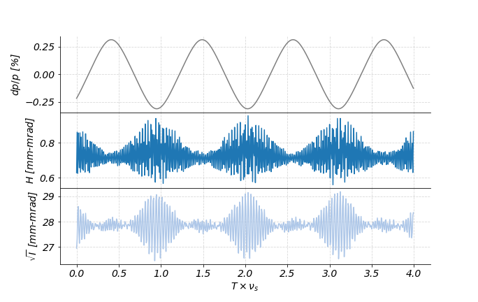
This periodicity is consistent over many hundreds of synchrotron periods, and across many initial particle trajectories. That persistence without secular growth indicates the presence of stroboscopic invariants in the Danilov-Nagaitsev Hamiltonian with synchrotron motion and chromatic effects, as applied to the iRCS lattice.

We have presented an approach to computing the $N$-turn map for an entire synchrotron period, and derived a stroboscopic Hamiltonian $\overline{H}$ which defines the secular Hamiltonian dynamics of the full synchro-betatron coupling. The stroboscopic Hamiltonian is the average of the transverse Hamiltonian over a synchrotron period. This Hamiltonian is $\mathcal{O}(\nu_{s}^{-1})$, with $\nu_{s}\ll 1$ the synchrotron tune, while the correction terms remain $\mathcal{O}(1)$. Therefore, this holds well for small synchrotron tune. Furthermore, for multi-synchrotron-period maps, these correction terms will oscillate with the number of periods, while the stroboscopic Hamiltonian term will grow linearly, suggesting that it dominates the long-term dynamics. We presented evidence of this stroboscopic Hamiltonian in the context of an integrable optics rapid cycling synchrotron, showing that the on-momentum Danilov-Nagaitsev invariants vary with momentum offset, but are periodic with the synchrotron period. The result, however, is generic to any Hamiltonian for the transverse dynamics, so long as a single Hamiltonian which generates the single-turn map for the transverse dynamics exists, i.e. in the absence of chaos.

References

- Hammer et al. [1955] C. L. Hammer, R. W. Pidd, and K. M. Terwilliger. Betatron Oscillations in the Synchrotron. Rev. Sci. Instr., 26(555), 1955. doi: 10.1063/1.1715241.
- Yu. F. Orlov [1957] Yu. F. Orlov. Excitation of Betatron Oscillations by Synchrotron Momentum Oscillations in a Strong Focusing Accelerator. Soviet Phys. JETP, Vol: 5, 1957.
- Lee [1994] S. Y. Lee. Single particle dynamics at synchro-betatron coupling resonances. Phys. Rev. E, 49(5706), 1994. doi: 10.1103/PhysRevE.49.5706.
- Danilov and Nagaitsev [2010] V. Danilov and S. Nagaitsev. Nonlinear accelerator lattices with one and two analytic invariants. Phys. Rev. ST Acc. Beams, 13(084002), 2010.
- Nagaitsev et al. [2010] S. Nagaitsev, A. Valishev, and V. Danilov. Nonlinear optics as a path to high-intensity circular machines. In Proceedings of HB2010, number THO1D01, 2010.
- Nagaitsev and Danilov [2010] S. Nagaitsev and V. Danilov. A search for integrable four-dimensional nonlinear accelerator lattices. In Proceedings of IPAC ’10, number THPE094, 2010.
- Nagaitsev and Valishev [2010] S. Nagaitsev and A. Valishev. Description of nonlinear elements for the integrable optics test accelerator. FNAL Note, Nov. 2010.
- Dragt and Abell [1996] A. Dragt and D. T. Abell. Symplectic Maps and Computation of Orbits in Particle Accelerators. In J. E. Marsden, G. W. Patrick, and W. F. Shadwick, editors, Integration Algorithms and Classical Mechanics, volume 10. American Mathematical Society, 1996.
- Dragt and Finn [1976] A. Dragt and J. Finn. Lie series and invariant functions for analytic symplectic maps. J. Math. Phys., 17(12), 1976.
- Dragt and Forest [1983] A. Dragt and E. Forest. Computation of nonlinear behavior of Hamiltonian systems using Lie algebraic methods. J. Math. Phys., 24(12), 1983.
- Dragt [2016] A. Dragt. Lie Methods for Nonlinear Dynamics with Applications to Accelerator Physics. University of Maryland, 2016.
- Dragt [1979] A. Dragt. A Method of Transfer Maps for Linear and Nonlinear Beam Elements. IEEE Trans. Nucl. Sci., NS-26(3), 1979.
- Dragt [1982] Alex J. Dragt. Lectures on nonlinear orbit dynamics. In Physics of High Energy Particle Accelerators, volume 87, pages 147–313. AIP Publishing, 1982.
- Dragt [1984] A. J. Dragt. Nonlinear lattice functions. In R. Donaldson and J. Morfín, editors, Proceedings of the 1984 Summer Study on the Design and Utilization of the Superconducting Super Collider, pages 369–372, 1984.
- Forest [1998] É. Forest. Dispersive lattice functions in a six-dimensional pseudo-harmonic-oscillator. Phys. Rev. E, 58(2):2481–2488, 1998.
- Arnold [1988] V. I. Arnold. Geometrical Methods in the Theory of Ordinary Differential Equations. Springer, 1988.
- Yoshida [1990] H. Yoshida. Construction of higher order symplectic integrators. Phys. Lett. A, 150(5-7):262–268, 1990.
- Lichtenberg and Lieberman [1992] A. J. Lichtenberg and M. A. Lieberman. Regular and Chaotic Dynamics. Springer-Verlag, 1992.
- Eldred and Valishev [2017] J. Eldred and A. Valishev. Integrable RCS as a proposed replacement for the Fermilab Booster. In AIP Conf. Proc., volume 1812, 2017. doi: 10.1063/1.4975901.
- Webb et al. [2015] S. D. Webb, D. L. Bruhwiler, S. Nagaitsev, A. Valishev, and V. V. Danilov. Chromaticity and Dispersion in Nonlinear Integrable Optics. In Proc. of 6th Intl. Particle Accelerator Conference, 2015.