Optimization by moving ridge functions:
Derivative-free optimization for computationally intensive functions

For standard trust region methods, a common choice of model is the Taylor series expansion centred around $\mathbf{x}_{k}$

where $\mathbf{B}_{k}$ is a symmetric matrix approximating the Hessian $\nabla^{2}f(\mathbf{x}_{k})$. Constructing this Taylor quadratic clearly requires knowledge of the function derivatives. Alternatively, DFTR methods may use interpolation or regression to construct $m_{k}$. That is, using a set of $p$ samples $\mathcal{X}=\{\mathbf{x}^{1},\mathbf{x}^{2},\dots,\mathbf{x}^{p}\}$ and $q$ basis functions $\phi(\mathbf{x})=\{\phi_{1}(\mathbf{x}),\dots,\phi_{q}(\mathbf{x})\}$, the model is defined as

where $\alpha_{j}$ for $j=1,\dots,q$ are the coefficients of the model. In the case of fully-determined interpolation, the number of samples is equal to the number of coefficients, i.e. $p=q$, so the coefficients may be determined by solving the linear system

where

Note that the current iterate $\mathbf{x}_{k}$ is generally included in the interpolation set, so $\mathbf{x}^{1}=\mathbf{x}_{k}$.

Global convergence of trust region methods which use the Taylor quadratic (6) has been proven (Conn, Gould, and Toint 2000). These convergence properties rely heavily on the well-understood error bounds for Taylor series. For these same guarantees to hold for DFTR methods, one must ensure the surrogate models satisfy Taylor-like error bounds

for all $\mathbf{x}\in B(\mathbf{x}_{k},\Delta_{k})$, where $\kappa_{1},\kappa_{2}>0$ are independent of $\mathbf{x}_{k}$ and $\Delta_{k}$. Models which satisfy these conditions are known as fully linear. A similar definition exists for fully quadratic models, i.e. models which have similar convergence properties as a second-order Taylor series.

Satisfying certain geometric conditions on the sample set $\mathcal{X}$ (Conn, Scheinberg, and Vicente 2008) allows one to ensure fully linear/quadratic models. In the case of polynomial surrogates, Conn, Scheinberg, and Vicente 2009b proved that these conditions on $\mathcal{X}$ were equivalent to bounding the condition number of the matrix

where

In particular, it was shown that, if the condition number of $\tilde{\mathbf{M}}$ is sufficiently bounded, then polynomial models constructed from $\mathcal{X}=\{\mathbf{x}^{1},\mathbf{x}^{2},\dots,\mathbf{x}^{p}\}$ are fully linear/quadratic. Numerous algorithms for improving the geometry of $\mathcal{X}$ for polynomial interpolation are presented by Conn, Scheinberg, and Vicente 2009b (see Chapter 6).

Fully-determined polynomial interpolation of degree $r$ in $n$ dimensions requires $p={n+r\choose r}$ function evaluations. In the case of quadratic interpolation, this would require $p=\frac{1}{2}(n+1)(n+2)$ sample points. When $n$ is small, this requirement may be easily met; however, as $n$ increases, this requirement may become prohibitive, particularly in the case of functions which are expensive to evaluate. Many DFTR methods account for this computational burden by avoiding the use of fully-determined quadratic models. For instance, the optimization algorithm COBYLA (Powell 1994) uses linear models, requiring only $n+1$ samples. Although this greatly reduces the effect of increased dimensionality, linear models generally do not capture the curvature of the true function, so convergence may be slow (Wendor, Botero, and Alonso 2016).

Some algorithms reduce the required number of samples by constructing under-determined quadratic interpolation models. This requires more samples than is necessary for linear models, but fewer than fully-determined quadratic models. For example, the algorithms NEWUOA (Powell 2006) and BOBYQA (Powell 2009) use minimum Frobenius norm interpolating quadratics, which require a constant number of more than $n+1$ points, but less than $\frac{1}{2}(n+1)(n+2)$ points. Generally, a default of $2n+1$ is used. Many other optimization algorithms (Zhang, Conn, and Scheinberg 2010; Cartis et al. 2019) have used a similar approach, and it has proven to be quite effective in practice. Nevertheless, this initial requirement may limit the efficacy of these approaches when the objective is both high-dimensional and computationally expensive.

Alternatively, other DFTR algorithms seek to reduce the initial start-up cost by using very few points initially, but increasing the number of points as more become available. For example, the DFO-TR algorithm proposed by Bandeira, Scheinberg, and Vicente 2012 builds quadratic models using significantly fewer than $\frac{1}{2}(n+1)(n+2)$ points, possibly as few as $n+1$ points. Although this was done using minimum Frobenius norm models, as in NEWUOA and BOBYQA, they also showed that, by assuming approximate Hessian sparsity, one could also use sparsity recovery techniques, such as compressed sensing (Eldar and Kutyniok 2012). Furthermore, it was proven that such models are probabilistically fully quadratic. That is, these models satisfy second-order Taylor-like error bounds with a probability bounded below by a term dependent on the number of sample points used. Moreover, the convergence of DFTR methods which employ probabilistically fully linear/quadratic models was proved by Bandeira, Scheinberg, and Vicente 2014, provided the models satisfied the Taylor-like error bounds with probability greater than or equal to $\frac{1}{2}$.

The active subspace of a given function $f(\mathbf{x})$ has been defined by Constantine, Dow, and Wang 2014 as the $d$-dimensional subspace $\mathbf{U}\in\mathbb{R}^{n\times d}$ of the inputs $\mathbf{x}\in\mathbb{R}^{n}$ which corresponds to the directions of strongest variability of $f$. To see how one may discover $\mathbf{U}$, consider a probability density function $\rho(\mathbf{x})$ which is strictly positive on the domain of interest and assume that

where $\mathbf{I}$ is the $n\times n$ identity matrix. Provided $\int\mathbf{x}\mathbf{x}^{T}\rho(\mathbf{x})d\mathbf{x}$ is full rank, these assumptions are easily satisfied by a change of variables (Constantine and Doostan 2017). Typically, $\rho(\mathbf{x})$ is taken to be Gaussian for unbounded inputs $\mathbf{x}$, with each coordinate scaled and shifted to be of mean 0 and standard deviation 1. When $\mathbf{x}$ is bounded below and above, $\rho(\mathbf{x})$ is generally taken to be the uniform distribution with $\mathbf{x}$ scaled and shifted to lie between $[-1,1]^{n}$.

Given $f$ and its partial derivatives are square integrable with respect to $\rho(\mathbf{x})$, the active subspace of $f$ can be found using the covariance matrix

In practice, this covariance matrix is approximated by

where $\mathbf{x}_{i}$ are drawn randomly from $\rho(\mathbf{x})$. This matrix is symmetric, positive semidefinite, so its real eigendecomposition is given by

where $\mathbf{\Lambda}=\text{diag}(\lambda_{1},\dots,\lambda_{d},\dots,\lambda_{n})$ and $\lambda_{1}\geq\dots\geq\lambda_{d}\geq\dots\lambda_{n}\geq 0$. Partitioning $\mathbf{W}$ and $\mathbf{\Lambda}$ as

results in the active subspace $\mathbf{U}\in\mathbb{R}^{n\times d}$ and the inactive subspace $\mathbf{V}\in\mathbb{R}^{n\times(n-d)}$. The reduced coordinates $\mathbf{y}=\mathbf{U}^{T}\mathbf{x}$ and $\mathbf{z}=\mathbf{V}^{T}\mathbf{x}$ are known as the active and inactive variables, respectively. The following lemma quantifies the variation of $f$ along these coordinates.

From Lemma 3.1 it is clear that on average $f$ shows greater variability along $\mathbf{y}$ than $\mathbf{z}$. Moreover, the sum of the partitioned eigenvalues $\mathbf{\Lambda}_{1}$ and $\mathbf{\Lambda}_{2}$ quantifies this variation. This motivates the well-known heuristic of choosing the reduced dimension $d$ as the index with the greatest log decay of eigenvalues (Constantine 2015).

In the derivative-free context, the approximate covariance matrix

where $\hat{f}$ is a surrogate model of $f$, may be used as a surrogate for $\mathbf{C}$. The efficacy of this approach is clearly dependent on the accuracy of the inferred gradients. To provide a theoretical guarantee of this statement, assume that

for all $\mathbf{x}\in B$ for some domain $B$ with $\omega_{h}$ independent of $\mathbf{x}$ and

where $\hat{f}$ is a surrogate model for $f$ and $h$ is some controllable parameter. Note, if $\hat{f}$ is fully linear, then by definition,

implying that fully linear models inherently satisfy this assumption as $\Delta_{k}\rightarrow 0$, i.e. as the trust region radius shrinks. Given this assumption, the following lemma (modified from Lemma 3.11 in Constantine 2015) provides an error bound between the approximate covariance matrix $\hat{\mathbf{C}}$ (18) and the true covariance matrix $\mathbf{C}$ (13).

Provided $\nabla\hat{f}(\mathbf{x})$ is easily computed, one may be able to compute an analytic form for $\hat{\mathbf{C}}$. Two model-based heuristics for approximating active subspaces using $\hat{\mathbf{C}}$, one with $\hat{f}$ a quadratic model and one a linear model, were proposed by Constantine and Doostan 2017 (see Algorithms 1 and 2). In the case of a quadratic model

using the assumptions on $\rho(\mathbf{x})$ from (12), the approximate covariance matrix (18) becomes

The active subspace $\mathbf{U}$ can then be approximated by partitioning the eigenvectors of $\hat{\mathbf{C}}$ by the log decay of its eigenvalues, as before. In the case of a linear model

the approximate covariance matrix (18) becomes

so the active subspace may be approximated by the 1-dimensional vector

These model-based heuristics have been successfully applied to a number of real-life applications. For instance, active subspaces for models of lithium ion batteries (Constantine and Doostan 2017) and turbomachinery models (Seshadri et al. 2018) have been approximated in this way. Moreover, this approach offers significant benefits over other subspace-based dimension reduction strategies. First, it is completely derivative-free. This allows it to be easily incorporated with other DFTR methods to reduce the computational overhead of surrogate modeling. Second, provided the inferred gradients satisfy the assumption (19), the error between the approximate covariance matrix (18) and the true covariance matrix (13) may be bounded using Lemma 3.2. Finally, calculating the approximate 1-dimensional subspace (25) is very inexpensive compared to other methods, requiring only $n+1$ samples to approximate the active subspace. However, one major limitation of this approach is that (25) can only be used to approximate a 1-dimensional active subspace. When the function of interest is not sufficiently described using a single direction, this approach may fail. Although the global quadratic covariance matrix (22) has been effectively used to calculate higher dimensional subspaces (Seshadri et al. 2018), it also requires a significant overhead in function evaluations. This limitation motivates the use of an alternative method of ridge function approximation in the case where higher dimensional subspaces are desired.

Unlike the active subspaces approach, ridge function recovery allows one to find the subspace $\mathbf{U}$ and the coefficients $\boldsymbol{\alpha}$ (7) of a ridge function $m(\mathbf{U}^{T}\mathbf{x})$ simultaneously. Hokanson and Constantine 2017 developed a method of doing this for the case in which $m$ is a polynomial of dimension $d$ and degree $r$. Their approach was to use variable projection to solve the minimization problem

where $\mathbb{P}^{r}(\mathbb{R}^{d})$ denotes the set of polynomials on $\mathbb{R}^{d}$ of degree $r$, $\mathbb{G}(d,\mathbb{R}^{n})$ denotes the Grassmann manifold of $d$-dimensional subspaces of $\mathbb{R}^{n}$, and $\{\mathbf{x}^{i}\}$ is a set of $M$ samples. Writing $m(\mathbf{U}^{T}\mathbf{x}^{i})$ as

(as seen in (8)), where $\mathcal{Y}=\{\mathbf{U}^{T}\mathbf{x}^{i}\mid i=1,\dots,M\}$, allows one to formulate (26) as a nonlinear least squares problem in terms of the coefficients $\boldsymbol{\alpha}$ and the subspace $\mathbf{U}$

with $\mathbf{f}\in\mathbb{R}^{M}$ such that $f_{i}=f(\mathbf{x}^{i})$ and $q={d+r\choose r}$. Using the fact that $\boldsymbol{\alpha}$ may be easily discovered using the Moore-Penrose pseudoinverse, one may write (27) as the Grassmann manifold optimization problem

over strictly $\mathbf{U}$. To solve this problem, Hokanson and Constantine 2017 developed a novel Grassmann Gauss-Newton method for iteratively solving (28).

Global convergence of DFTR methods relies on models which are fully linear, i.e. models which satisfy the bounds (10). Demonstrating full linearity of ridge function models $m(\mathbf{U}^{T}\mathbf{x})$ requires

for all $\mathbf{x}\in B(\mathbf{x}_{k},\Delta)$ (4), where $\kappa_{1},\kappa_{2}$ are constants which are independent of $\mathbf{x}$ and $\Delta$. For standard polynomial interpolation models, one may use well poisedness of the interpolation set to prove full linearity (as shown in Conn, Scheinberg, and Vicente 2008). However, in the case of polynomial ridge functions, there is an extra level of complexity involved as the models are constructed over a projected input space. Unless $f$ has an exact ridge function representation with known effective dimension, projection of its domain onto the subspace $\mathbf{U}$ will have some inherent information loss associated with it. This is because, for each value of the reduced coordinate $\mathbf{y}$, there exist many (possibly infinitely many) coordinates in the full space which map to it. Variations in the function values associated with each full space coordinate may show up as ‘noise’ in the $d$-dimensional projection of the function domain. This observation leads to two forms of error: 1) information loss from dimension reduction, and 2) response surface error which arises from polynomial interpolation with samples which are corrupted by noise.

To formalize these two forms of error, consider the conditional expectation of $f$ given $\mathbf{y}=\mathbf{U}^{T}\mathbf{x}$.

That is, the conditional expectation of $f$ given $\mathbf{y}$ is the average value of $f(\mathbf{x})$ for all possible values $\mathbf{x}$ for a given reduced coordinate $\mathbf{y}=\mathbf{U}^{T}\mathbf{x}$. The function $g(\mathbf{y})$ is the unique, optimal ridge function approximation in the $L^{2}(\rho)$ norm for a given subspace $\mathbf{U}$ (see the proof of Theorem 8.3 in Pinkus 2015).

The error functions

represent the information loss from reducing onto the subspace $\mathbf{U}$. If one can appropriately bound $|e^{g}(\mathbf{x})|$ and $\|\mathbf{e}^{g}(\mathbf{x})\|$ for all $\mathbf{x}\in B(\mathbf{x}_{k},\Delta)$, one can show full linearity of the conditional expectation $g$ (30). Although the mean-squared error of $g$ with respect to $f$ is known to be bounded in expectation (see Theorem 3.1 by Constantine, Dow, and Wang 2014), there exists no formal error analysis for bounding the error functions (31) for any $f$ and $\mathbf{U}$. However, in the special case where $f$ has no dependence on $\mathbf{z}$, these error bounds are satisfied. Such functions are known as $\mathbf{z}$-invariant. Using the following proposition proposed by Constantine 2015, full linearity of $g$ is trivially shown in the case where $f$ is $\mathbf{z}$-invariant.

Unfortunately, using $g(\mathbf{y})$ as a surrogate model is not practical, as it requires high-dimensional integration along the $\mathbf{z}$ coordinate. Instead, a ridge function approximation $m(\mathbf{y})$ which acts as a surrogate to $g$ is used. This introduces the error functions

which represent the response surface error. Although $g$ may be smooth and differentiable with respect to reduced coordinates $\mathbf{y}$, the $d$-dimensional samples used to construct $m$ will be noisy as they will be obtained from the $n$-dimensional function $f$. Kannan and Wild 2012 provide theoretical guarantees for quadratic models constructed from noisy functions (see Theorem 2.2). Using similar logic, the following theorem provides error bounds for $|e^{m}(\mathbf{y})|$ and $\|\mathbf{e}^{m}(\mathbf{y})\|$.

The majority of research into ridge function approximations has assumed that the function of interest varies along a global subspace $\mathbf{U}$ (Glaws et al. 2017; Wong et al. 2019; Gross, Seshadri, and Parks 2020). Unless the function is an exact ridge function, i.e. $f$ is $\mathbf{z}$-invariant, this assumption may lead to a significant amount of information loss when projecting onto the subspace. However, using local subspaces $\{\mathbf{U}_{k}\}$, with each $\mathbf{U}_{k}$ corresponding to a small region of interest in the function domain, may allow $f$ to be accurately modeled as a $\mathbf{z}$-invariant function. To motivate this approach, six 10-dimensional functions from the CUTEst (Gould, Orban, and Toint 2015) problem set have been considered (ARGLINA, MCCORMCK, NCVXBQP1, PENALTY1, SCHMVETT, VARDIM). For each of these functions, active subspaces have been approximated using the Monte-Carlo gradient sampling method (14) with 100,000 samples taken at uniformly distributed random locations. The active subspaces for six regions of interest defined by hypercubes of variable radius $\Delta$, all centred at the same randomly chosen location in the function domain were calculated. The eigenvalues for each of these functions are shown in Figure 1.

From inspection of Figure 1, it is apparent that, as $\Delta$ decreases, the gap between the first eigenvalue and the remaining eigenvalues generally increases for these functions. This suggests that, as the region of interest becomes smaller, these functions become inherently 1-dimensional. Moreover, for many of these functions the remaining eigenvalues seem to tend to zero as $\Delta$ decreases. By Lemma 3.1, this implies very little to no average variability along the inactive variables $\mathbf{z}$, meaning these functions can be treated as nearly $\mathbf{z}$-invariant for small $\Delta$. Note, there clearly exist functions which seemingly do not have eigenvalues which tend to zero. For instance, although VARDIM has seemingly very strong 1-dimensional structure at this particular location in the function domain, the remaining eigenvalues are still $\mathcal{O}(10^{12})$. This suggests that at this particular region of the domain, although VARDIM has strong 1-dimensional structure, this structure does not get more prominent as the size of function domain decreases.

In order to use dimension-reducing subspaces in a DFTR algorithm, it is hypothesized that the subspaces should be periodically updated as one moves through the function domain. To motivate this hypothesis, local active subspaces for six regions have been defined by hypercubes of radius $\Delta=1.0\times 10^{-3}$ for each function. The centroids of the hypercubes were chosen using Latin hypercube sampling such that each local region was sufficiently distant from the others. The eigenvalues of these subspaces are shown in Figure 2.

For each of these functions, one can see a significant log decay in the eigenvalues after the first index for all of the local subspaces. This suggests that, for each of these regions of interest, the direction defined by the first eigenvector of (14) captures a significant amount of the variation of the function. Note, the observation that, in small regions of interest, multivariate functions can be approximated by 1-dimensional ridge functions is not surprising. In particular, the first-order Taylor expansion

can be considered a 1-dimensional ridge function with the subspace $\mathbf{U}=\nabla f(\mathbf{a})$. However, this observation clearly breaks down when considering subspaces of higher dimension. Nevertheless, using subspaces of higher dimension may still be advantageous for some problems, as will be seen later.

The weights from each of these 1-dimensional subspaces are shown in Figure 3, with the size of the markers indicating the relative size of the weights. Not surprisingly, the weight vectors generally vary significantly between each region of interest. Clearly, it would be nearly impossible to accurately describe these functions with constant subspaces, as there are regions which have a weight vector which is linearly independent of the weight vectors associated with other regions of the function domain. Interestingly, some functions seem to have multiple regions of the function domain which can be defined using a single subspace. For instance, it looks to be possible to define these six regions of interest for the SCHMVETT function by 3 low-dimensional subspaces, one using strictly the 9th parameter, another using the 10th parameter, and one with a mixture of the two. This observation may motivate the use of subspace clustering techniques (Parsons, Haque, and Liu 2004) in further studies.

In Section 3.3, it was shown that the accuracy of a ridge function model $m_{k}$ is dependent on two sources of error: information loss by projecting onto a subspace $\mathbf{U}_{k}$ and the response surface error of $m_{k}$. Ideally, a single interpolation set could be maintained which could be improved to reduce both sources of error. Unfortunately, such an approach would require a priori knowledge of the subspace $\mathbf{U}_{k}$. Therefore, OMoRF maintains two separate interpolation sets: $\mathcal{X}_{k}^{sub}$ of $n+1$ samples for calculating $\mathbf{U}_{k}$, and $\mathcal{X}_{k}^{int}$ of $\frac{1}{2}(d+1)(d+2)$ samples for calculating the coefficients of $m_{k}$.

The set $\mathcal{X}_{k}^{sub}$ is used to construct the subspace $\mathbf{U}_{k}$ using either derivative-free active subspaces or polynomial ridge approximation. In either case, the first step is to build a fully linear $n$-dimensional linear interpolator $\hat{f}$ (23). In the case of derivative-free active subspaces, $\mathbf{U}_{k}$ is simply the 1-dimensional active subspace (25). If a greater dimensionality is required, $\mathcal{X}_{k}^{sub}$ is used to solve the Grassmann manifold optimization problem (28). Note, solving (28) requires an initial guess for $\mathbf{U}_{k}$. In OMoRF, the approximate 1-dimensional subspace (25), appended with its orthogonal complement, is used as the initial point for the manifold optimization problem (28). Note, although the solution to problem (28) could also be used in the case of $d=1$, it was found that the 1-dimensional active subspace (25) generally gave superior algorithmic performance. Therefore, this method is only employed in the case where higher dimensions are desired, e.g. when it is believed that a 1-dimensional subspace insufficiently describes the underlying problem dimension.

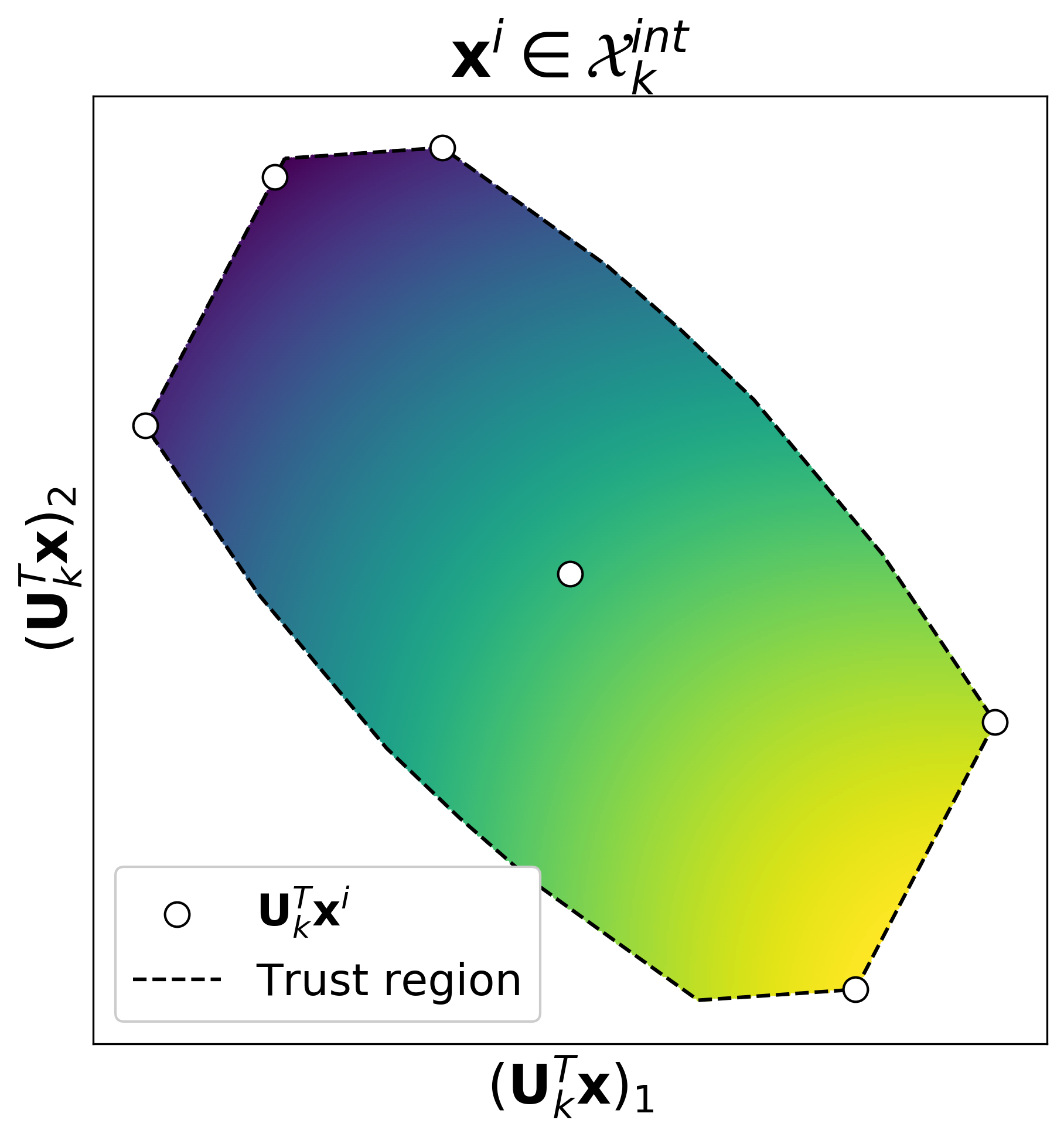
Once the subspace $\mathbf{U}_{k}$ is known, one may be tempted to use the points $\mathcal{Y}_{k}^{sub}=\{\mathbf{U}_{k}^{T}\mathbf{x}^{i}\mid\mathbf{x}^{i}\in\mathcal{X}_{k}^{sub}\}$ to calculate the coefficients of $m_{k}$. However, these projected samples generally insufficiently span the $d$-dimensional projected space, leading to poor surrogate models. Provided $d\ll n$, determining a more suitable set of $\frac{1}{2}(d+1)(d+2)$ samples $\mathcal{X}_{k}^{int}$ is not only relatively cheap, but can also dramatically improve the quality of the ridge function surrogate. Figure 4 provides an example of the 10-dimensional Styblinski-Tang function

projected onto a 2-dimensional subspace. From this figure it is clear that, although the set $\mathcal{X}_{k}^{sub}$ may be well suited for linear interpolation in 10 dimensions, the projected set $\mathcal{Y}_{k}^{sub}$ does not span the 2-dimensional space very well. In contrast, the projected set $\mathcal{Y}_{k}^{int}=\{\mathbf{U}_{k}^{T}\mathbf{x}^{i}\mid\mathbf{x}^{i}\in\mathcal{X}_{k}^{int}\}$ effectively spans this space, which in turn gives a much more accurate ridge function model. To demonstrate this increase in accuracy, $N=100,000$ samples $\hat{\mathbf{x}}_{i}$ were drawn at random from a uniform distribution bounded by the trust region domain. From these samples, the coefficient of determination

where

and $\bar{f}=\frac{1}{N}\sum_{i=1}^{N}f(\hat{\mathbf{x}}_{i})$, was calculated for both of these models. The $R^{2}$ values for the ridge function models constructed from $\mathcal{Y}_{k}^{sub}$ and $\mathcal{Y}_{k}^{int}$ can be seen in Figure 4.

Algorithm 1 always includes new sample points as they become available by appending $\mathbf{x}_{k}+\mathbf{s}_{k}$ to the interpolation sets $\mathcal{X}_{k}^{sub}$ and $\mathcal{X}_{k}^{int}$. When the iterate is successful, i.e. $r_{k}\geq\eta_{1}$, Algorithm 3 is invoked for both sample sets to choose a point to be replaced for each set before continuing the iteration. Note, new sample points are not calculated during this call of Algorithm 3. When the iterate is not successful, it is necessary to ensure the accuracy of the model before reducing the trust region radius $\Delta_{k}$. In this case, not only is the previously calculated sample added, but another new geometry-improving point is determined and subsequently added. Determining whether or not these sets need to be improved is done by checking the maximum distance of the samples to the current iterate. If this distance is too large, it indicates the interpolation set has not been updated recently, so it may need improvement. The full details of this process are provided in Algorithm 2.

There are a few points to note about Algorithm 2. First, although other conditions may be used as a measure of the quality of an interpolation set, the maximum distance of the samples to the current iterate gives a quick and simple means of determining whether or not to improve the interpolation set. Similar approaches have been successfully applied in other DFTR methods (Fasano, Morales, and Nocedal 2009; Bandeira, Scheinberg, and Vicente 2012; Cartis and Roberts 2019). Second, a pivotal algorithm, which has been modified from Algorithm 6.6 in Conn, Scheinberg, and Vicente 2009b, has been used both to choose points to be replaced and calculate new geometry-improving points. The details of this modified algorithm are given in Algorithm 3 in Appendix C. Third, to reduce the computational burden of each iteration, only a single geometry-improving sample point is calculated during calls of Algorithm 3. The point which is replaced by this new sample point is also determined using Algorithm 3. Fourth, improvements to $\mathcal{X}_{k}^{int}$ are prioritized over $\mathcal{X}_{k}^{sub}$. This is because $\mathcal{X}_{k}^{int}$ generally has significantly fewer samples than $\mathcal{X}_{k}^{sub}$, so $\mathcal{X}_{k}^{int}$ can be updated more rapidly than $\mathcal{X}_{k}^{sub}$. If all of the points in $\mathcal{X}_{k}^{int}$ are sufficiently close to the current iterate $\mathbf{x}_{k}$, this indicates that $\mathcal{X}_{k}^{int}$ has been recently improved. In these cases, if the model $m_{k}$ needs improving, it may be because the subspace $\mathbf{U}_{k}$ needs to be updated. Finally, a new subspace $\mathbf{U}_{k+1}$ is calculated whenever the geometry of $\mathcal{X}_{k}^{sub}$ is improved. This is because improving the geometry of $\mathcal{X}_{k}^{sub}$ improves the quality of the linear interpolator $\hat{f}$ (23), which, by Lemma 3.2, leads to a more accurate covariance matrix (18). Therefore, improving $\mathcal{X}_{k}^{sub}$ before calculating $\mathbf{U}_{k+1}$ potentially allows the algorithm to find a more suitable dimension-reducing subspace.

References

- Bandeira, Scheinberg, and Vicente (2012) Bandeira, Afonso, Katya Scheinberg, and Luís Vicente. 2012. “Computation of sparse low degree interpolating polynomials and their application to derivative-free optimization.” In Mathematical Programming, Vol. 134, 223–257.
- Bandeira, Scheinberg, and Vicente (2014) Bandeira, Afonso, Katya Scheinberg, and Luís Vicente. 2014. “Convergence of trust-region methods based on probabilistic models.” SIAM Journal on Optimization 24 (3): 1238–1264.
- Bergstra and Bengio (2012) Bergstra, James, and Yoshua Bengio. 2012. “Random search for hyper-parameter optimization.” Journal of Machine Learning Research 13: 281–305.
- Cartis et al. (2019) Cartis, Coralia, Jan Fiala, Benjamin Marteau, and Lindon Roberts. 2019. “Improving the flexibility and robustness of model-based derivative-free optimization solvers.” ACM Transactions on Mathematical Software 45 (3): 1–41.
- Cartis and Otemissov (2020) Cartis, Coralia, and Adilet Otemissov. 2020. “A dimensionality reduction technique for unconstrained global optimization of functions with low effective dimensionality.” (Preprint).
- Cartis and Roberts (2019) Cartis, Coralia, and Lindon Roberts. 2019. “A derivative-free Gauss-Newton method.” Mathematical Programming Computation 11 (4): 631–674.
- Choromanski et al. (2019) Choromanski, Krzysztof, Aldo Pacchiano, Jack Parker-Holder, Yunhao Tang, and Vikas Sindhwani. 2019. “From complexity to simplicity: Adaptive ES-active subspaces for blackbox optimization.” In Advances in Neural Information Processing Systems, 10299–10309.
- Conn, Gould, and Toint (2000) Conn, Andrew, Nicholas Gould, and Philippe Toint. 2000. Trust-region methods. Philadelphia, Pa.: Society for Industrial and Applied Mathematics: Mathematical Programming Society.
- Conn, Scheinberg, and Vicente (2008) Conn, Andrew, Katya Scheinberg, and Luís Vicente. 2008. “Geometry of interpolation sets in derivative free optimization.” Mathematical Programming 111 (1): 141–172.
- Conn, Scheinberg, and Vicente (2009a) Conn, Andrew, Katya Scheinberg, and Luís Vicente. 2009a. “Global convergence of general derivative-free trust-region algorithms to first- and second-order critical points.” SIAM Journal on Optimization 20 (1): 387–415.
- Conn, Scheinberg, and Vicente (2009b) Conn, Andrew, Katya Scheinberg, and Luís Vicente. 2009b. Introduction to derivative-free optimization. Philadelphia, Pa.: Society for Industrial and Applied Mathematics: Mathematical Programming Society.
- Constantine and Doostan (2017) Constantine, Paul, and Alireza Doostan. 2017. “Time-dependent global sensitivity analysis with active subspaces for a lithium ion battery model.” Statistical Analysis and Data Mining 10 (5): 243–262.
- Constantine, Dow, and Wang (2014) Constantine, Paul, Eric Dow, and Qiqi Wang. 2014. “Active subspace methods in theory and practice: Applications to kriging surfaces.” SIAM Journal on Scientific Computing 36 (4): A1500–A1524.
- Constantine (2015) Constantine, Paul G. 2015. Active subspaces: Emerging ideas for dimension reduction in parameter studies. Philadelphia, Pa.: SIAM Spotlights.
- Diez, Campana, and Stern (2015) Diez, Matteo, Emilio Campana, and Frederick Stern. 2015. “Design-space dimensionality reduction in shape optimization by Karhunen-Loève expansion.” Computer Methods in Applied Mechanics and Engineering 283 (1): 1525–1544.
- Eldar and Kutyniok (2012) Eldar, Yonina, and Gitta Kutyniok. 2012. Compressed sensing: Theory and applications. Cambridge, UK: Cambridge University Press.
- Fasano, Morales, and Nocedal (2009) Fasano, Giovanni, José Luis Morales, and Jorge Nocedal. 2009. “On the geometry phase in model-based algorithms for derivative-free optimization.” Optimization Methods and Software 24 (1): 145–154.
- Ghanbari and Scheinberg (2017) Ghanbari, Hiva, and Katya Scheinberg. 2017. “Black-box optimization in machine learning with trust region based derivative free algorithm.” (Preprint).
- Glaws et al. (2017) Glaws, Andrew, Paul Constantine, John N. Shadid, and Tim Wildey. 2017. “Dimension reduction in MHD power generation models: Dimensional analysis and active subspaces.” Statistical Analysis and Data Mining: The ASA Data Science Journal 10: 312–325.
- Gould, Orban, and Toint (2015) Gould, Nicholas, Dominique Orban, and Philippe Toint. 2015. “CUTEst: a Constrained and Unconstrained Testing Environment with safe threads for mathematical optimization.” Computational Optimization and Applications 60 (3): 545–557.
- Gould and Scott (2016) Gould, Nicholas, and Jennifer Scott. 2016. “A note on performance profiles for benchmarking software.” ACM Transactions on Mathematical Software 43 (2): 1–5.
- Gross, Seshadri, and Parks (2020) Gross, James, Pranay Seshadri, and Geoffrey Parks. 2020. “Optimisation with intrinsic dimension reduction: A ridge informed trust-region method.” In Proceedings of AIAA SciTech Forum and Exposition, Orlando, USA.
- Gu (2001) Gu, Lei. 2001. “A comparison of polynomial based regression models in vehicle safety analysis.” In Proceedings of the ASME Design Engineering Technical Conference, Vol. 2.
- Hokanson and Constantine (2017) Hokanson, Jeffrey, and Paul Constantine. 2017. “Data-driven polynomial ridge approximation using variable projection.” SIAM Journal on Scientific Computing 40 (3): 1566–1589.
- Johnson (2018) Johnson, Steven. 2018. “The NLopt nonlinear-optimization package.” http://github.com/stevengj/nlopt.
- Kannan and Wild (2012) Kannan, Aswin, and Stefan Wild. 2012. Obtaining quadratic models of noisy functions. Technical Report. 9700 South Cass Avenue, Argonne, Illinois, USA: Argonne National Labratory.
- Kipouros et al. (2008) Kipouros, Timoleon, Daniel Jaeggi, William Dawes, Geoffrey Parks, Mark Savill, and John Clarkson. 2008. “Biobjective design optimization for axial compressors using tabu search.” AIAA Journal 46 (3): 701–711.
- Kozak et al. (2019) Kozak, David, Stephen Becker, Alireza Doostan, and Luis Tenorio. 2019. “Stochastic subspace descent.” (Preprint).
- Levina et al. (2009) Levina, Tatsiana, Yuri Levin, Jeff McGill, and Mikhail Nediak. 2009. “Dynamic pricing with online learning and strategic consumers: An application of the aggregating algorithm.” Operations Research 57 (2): 327–341.
- Lukaczyk et al. (2014) Lukaczyk, Trent, Paul Constantine, Francisco Palacios, and Juan Alonso. 2014. “Active Subspaces for Shape Optimization.” In 10th AIAA Multidisciplinary Design Optimization Specialist Conference, .
- Moré and Wild (2009) Moré, Jorge, and Stefan Wild. 2009. “Benchmarking derivative-free optimization algorithms.” SIAM Journal on Optimization 20 (1): 172–191.
- Nelder and Mead (1965) Nelder, John, and Roger Mead. 1965. “A simplex method for function minimization.” The Computer Journal 7 (4): 308–313.
- Palacios et al. (2013) Palacios, Francisco, Michael Colonno, Aniket Aranake, Alejandro Campos, Sean Copeland, Thomas Economon, Amrita Lonkar, Trent Lukaczyk, Thomas Taylor, and Juan Alonso. 2013. “Stanford University Unstructured (SU2): An open-source integrated computational environment for multi-physics simulation and design.” In 51st AIAA Aerospace Sciences Meeting including the New Horizons Forum and Aerospace Exposition 2013, .
- Palacios and Kline (2017) Palacios, Francisco, and Heather Kline. 2017. “Constrained shape design of a transonic inviscid wing.” Accessed 2019-08-12. https://su2code.github.io/tutorials/Inviscid{_}3D{_}Constrained{_}ONERAM6/.
- Parsons, Haque, and Liu (2004) Parsons, Lance, Ehtesham Haque, and Huan Liu. 2004. “Subspace Clustering for High Dimensional Data: A Review.” SIGKDD Explorations, Newsletter of the ACM Special Interest Group on Knowledge Discovery and Data Mining 6 (1): 90–105.
- Pinkus (2015) Pinkus, Allan. 2015. Ridge functions. Cambridge, UK: Cambridge University Press.
- Powell (1994) Powell, Michael. 1994. “A direct search optimization method that models the objective and constraint functions by linear interpolation.” In Advances in Optimization and Numerical Analysis, 51–67. Springer Netherlands.
- Powell (2006) Powell, Michael. 2006. “The NEWUOA software for unconstrained optimization without derivatives.” In Large-Scale Nonlinear Optimization, 255–297.
- Powell (2009) Powell, Michael. 2009. The BOBYQA algorithm for bound constrained optimization without derivatives. Technical Report. Cambridge, UK: Department of Applied Mathematics and Theoretical Physics, University of Cambridge.
- Qiu et al. (2018) Qiu, Yasong, Junqiang Bai, Nan Liu, and Chen Wang. 2018. “Global aerodynamic design optimization based on data dimensionality reduction.” Chinese Journal of Aeronautics 31 (4): 643–659.
- Scheinberg and Toint (2010) Scheinberg, Katya, and Philippe Toint. 2010. “Self-correcting geometry in model-based algorithms for derivative-free unconstrained optimization.” SIAM Journal on Optimization 20 (6): 3512–3532.
- Seshadri and Parks (2017) Seshadri, Pranay, and Geoffrey Parks. 2017. “Effective-Quadratures (EQ): Polynomials for computational engineering studies.” The Journal of Open Source Software 2 (11).
- Seshadri et al. (2018) Seshadri, Pranay, Shahrokh Shahpar, Paul Constantine, Geoffrey Parks, and Mike Adams. 2018. “Turbomachinery active subspace performance maps.” Journal of Turbomachinery 140 (4): 041003–1–041003–11.
- Shan and Wang (2010) Shan, Songqing, and G. Gary Wang. 2010. “Survey of modeling and optimization strategies to solve high-dimensional design problems with computationally-expensive black-box functions.” Structural and Multidisciplinary Optimization 41 (2): 219–241.
- Virtanen et al. (2020) Virtanen, Pauli, Ralf Gommers, Travis Oliphant, Matt Haberland, Tyler Reddy, David Cournapeau, Evgeni Burovski, et al. 2020. “SciPy 1.0: Fundamental algorithms for scientific computing in Python.” Nature Methods 17: 261–272.
- Wang et al. (2016) Wang, Ziyu, Frank Hutter, Masrour Zoghi, David Matheson, and Nando De Freitas. 2016. “Bayesian optimization in a billion dimensions via random embeddings.” Journal of Artificial Intelligence Research 55: 361–367.
- Wendor, Botero, and Alonso (2016) Wendor, Andrew, Emilio Botero, and Juan Alonso. 2016. “Comparing different off-the-shelf optimizers’ performance in conceptual aircraft design.” In 17th AIAA/ISSMO Multidisciplinary Analysis and Optimization Conference, .
- Wong et al. (2019) Wong, Chun Yui, Pranay Seshadri, Geoffrey Parks, and Mark Girolami. 2019. “Embedded ridge approximations: constructing ridge approximations over localized scalar fields for improved simulation-centric dimension reduction.” (Preprint).
- Zhang, Conn, and Scheinberg (2010) Zhang, Hongchao, Andrew Conn, and Katya Scheinberg. 2010. “A derivative-free algorithm for least-squares minimization.” SIAM Journal on Optimization 20 (6): 3555–3576.
- Zhao, Alimo, and Bewley (2018) Zhao, Muhan, Shahrouz Ryan Alimo, and Thomas Bewley. 2018. “An active subspace method for accelerating convergence in Delaunay-based optimization via dimension reduction.” In Proceedings of the IEEE Conference on Decision and Control, Miami Beach, Florida, USA, 2765–2770.
7 Appendices
Appendix A Proof of Lemma 3.2
Proof.
Let denote and denote . First, observe that
where is the Lipschitz constant of . Next,
Finally,
∎
Appendix B Proof of Theorem 3.5
Let
be a quadratic ridge function with and note
Subtracting from gives
Taking the first-order Taylor expansion of around and rearranging gives