跳到论文正文
W Papers独立论文阅读器 arXiv:2007.04787 论文正文 计算阅读时间 · 0%
引用这篇论文根据当前论文元数据生成,正式投稿前建议核对。


License: arXiv.org perpetual non-exclusive license
arXiv:2007.04787v1 [eess.SP] 08 Jul 2020

A Novel Heap-based Pilot Assignment for Full Duplex Cell-Free Massive MIMO with Zero-ForcingThis work was supported in part by the ERC project AGNOSTIC and FNR ECLECTIC.

Hieu V. Nguyen1, Van-Dinh Nguyen3, Octavia A. Dobre2, Shree Krishna Sharma3,
Symeon Chatzinotas3, Bjo¨\ddot{\text{o}}rn Ottersten3, and Oh-Soon Shin1
Affiliation: 1School of Electronic Engineering & Department of ICMC Convergence Technology, Soongsil University, Korea
2Faculty of Engineering and Applied Science, Memorial University, St. John’s, NL, Canada
3SnT, University of Luxembourg, L-1855 Luxembourg City, Luxembourg
Abstract

This paper investigates the combined benefits of full-duplex (FD) and cell-free massive multiple-input multiple-output (CF-mMIMO), where a large number of distributed access points (APs) having FD capability simultaneously serve numerous uplink and downlink user equipments (UEs) on the same time-frequency resources. To enable the incorporation of FD technology in CF-mMIMO systems, we propose a novel heap-based pilot assignment algorithm, which not only can mitigate the effects of pilot contamination but also reduce the involved computational complexity. Then, we formulate a robust design problem for spectral efficiency (SE) maximization in which the power control and AP-UE association are jointly optimized, resulting in a difficult mixed-integer nonconvex programming. To solve this problem, we derive a more tractable problem before developing a very simple iterative algorithm based on inner approximation method with polynomial computational complexity. Numerical results show that our proposed methods with realistic parameters significantly outperform the existing approaches in terms of the quality of channel estimate and SE.

I Introduction

In-band full-duplex (FD) has been envisaged as a key enabling technology to increase the spectral efficiency (SE) of a wireless link over its half-duplex (HD) counterparts by a factor close to two, since it allows downlink (DL) and uplink (UL) transmissions on the same time-frequency resources [1, 2, 3, 4]. Although the main barrier in implementing FD is the self-interference (SI), many recent advances in active and passive SI suppression techniques have been successful to bring the SI power at the background noise level [5]. As a result, FD-enabled base station (BS) systems have been widely studied in small-cell (SC) cellular networks [6, 7, 8, 9, 10].

Recently, cell-free massive multiple-input multiple-output (CF-mMIMO), where a very large number of access points (APs) is distributed over a wide area to coherently serve numerous user equipments (UEs) in the same resources, has been proposed to overcome the inter-cell interference [11, 12]. CF-mMIMO not only inherits the properties of favorable propagation and channel hardening from collocated massive MIMO networks (Co-mMIMO), but also reduces path losses due to the APs placed closer to UEs. It can be seen that the performance gains of CF-mMIMO are obtained by the joint process at a central processing unit (CPU).

Despite their potentials, there are only a few attempts on characterizing the performance of an FD-enabled CF-mMIMO. In this regard, the authors in [13] analyzed the performance of FD CF-mMIMO, where all APs operate in the FD mode with the usage of a conjugate beamforming/matched filtering transmission design. Tackling the imperfect channel state information (CSI) and spatial correlation for the FD CF-mMIMO system was studied in [14], with a genetic algorithm-based user scheduling strategy applied to alleviate the co-channel interference (CCI). However, none of the aforementioned works properly examined the training procedure for a practical purpose in FD CF-mMIMO, while the existing approaches designed for HD operation may not be inapplicable to FD operation under the strong effects of SI, inter-AP interference (IAI) and CCI. Moreover, it is crucial to develop a low-complexity robust design to attain the optimal SE performance of FD CF-mMIMO systems under channel uncertainties.

In the above context, this paper considers an FD CF-mMIMO system under time-division duplex (TDD) operation, where FD-enabled multiple-antenna APs simultaneously serve UL and DL UEs on the same time-frequency resources. A novel heap-based pilot assignment strategy for FD CF-mMIMO is proposed not only to enhance the quality of channel estimates but also to reduce the computational complexity required for the training process. Furthermore, we develop an efficient transmission design for FD CF-mMIMO, in which the power control and AP-DL UE association are jointly optimized to reduce network interference. Based on the widely-used zero-forcing (ZF) method, we propose a new robust design and an iterative algorithm whose complexity is less impacted by the large number of APs (or antennas). The main contributions of this paper are summarized as follows:

  • •

    We first propose a novel heap-based pilot assignment algorithm to reduce both pilot contamination and training complexity.

  • •

    Aiming at SE optimization, we introduce new binary variables to establish the AP-DL UE associations. In our system design, the APs can be automatically switched between the FD and HD operations, which allows to exploit the full potential of FD CF-mMIMO.

  • •

    We further consider a robust design problem for SE maximization with joint power control and AP-DL UE association, which is formulated as a difficult class of mixed-integer nonconvex optimization problem. To efficiently solve the problem, we first exploit the structure of the optimal solution of binary variables to transform the original problem into a more tractable form. Based on the ZF design, a very simple, yet efficient algorithm based on the inner approximation (IA) method is devised to obtain a locally optimal solution of the problem.

  • •

    Numerical results confirm that the proposed algorithms greatly reduce the pilot contamination and improve the SE performance over the current state-of-the-art approaches under both HD and FD operation modes.

Notation: 𝚃𝚛⁡(⋅){\mathtt{Tr}}(\cdot), ∥⋅∥\|\cdot\| and |⋅||\cdot| are the trace, Euclidean norm and absolute value, respectively. 𝚍𝚒𝚊𝚐⁡(𝐚)\mathtt{diag}(\mathbf{a}) returns the diagonal matrix with the main diagonal assembled from elements of 𝐚\mathbf{a}.

II System Model

II-A Transmission Model

Refer to caption
Fig. 1: An illustration of the full-duplex cell-free massive MIMO system.

An FD CF-mMIMO system operated in TDD mode is considered, where the set ℳ≜{1,2,⋯,M}\mathcal{M}\triangleq\{1,2,\cdots,M\} of MM FD-enabled APs simultaneously serves the sets 𝒦≜{1,2,⋯,K}\mathcal{K}\triangleq\{1,2,\cdots,K\} of KK DL UEs and ℒ≜{1,2,⋯,L}\mathcal{L}\triangleq\{1,2,\cdots,L\} of LL UL UEs in the same time-frequency resources, as illustrated in Fig. 1. The total number of APs’ antennas is N=∑m∈ℳNmN=\sum_{m\in\mathcal{M}}N_{m}, where NmN_{m} is the number of antennas at AP mm, while each UE has a single-antenna. All APs are equipped with FD capability by circulator-based FD radio prototypes [5], which are connected to the CPU through perfect backhaul links with sufficiently large capacities [11]. At the CPU, the message sent by an UL UE is decoded by aggregating the received signals from all active APs due to the UL broadcast transmission. Meanwhile, each DL UE should be served by a subset of active APs with good channel conditions [11]. This is done by introducing new binary variables to establish the AP-DL UE associations.

For notational convenience, let us denote the mm-th AP, kk-th DL UE and ℓ\ell-th UL UE by 𝙰𝙿m\mathtt{AP}_{m}, 𝚄k𝚍\mathtt{U}_{k}^{\mathtt{d}} and 𝚄ℓ𝚞\mathtt{U}_{\ell}^{\mathtt{u}}, respectively. The channel vectors and matrices from 𝙰𝙿m→𝚄k𝚍\mathtt{AP}_{m}\rightarrow\mathtt{U}_{k}^{\mathtt{d}}, 𝚄ℓ𝚞→𝙰𝙿m\mathtt{U}_{\ell}^{\mathtt{u}}\rightarrow\mathtt{AP}_{m}, 𝚄ℓ𝚞→𝚄k𝚍\mathtt{U}_{\ell}^{\mathtt{u}}\rightarrow\mathtt{U}_{k}^{\mathtt{d}} and 𝙰𝙿m′→𝙰𝙿m,∀m′∈ℳ\mathtt{AP}_{m^{\prime}}\rightarrow\mathtt{AP}_{m},\forall m^{\prime}\in\mathcal{M} are denoted by 𝐡k​m𝚍∈ℂ1×Nm\mathbf{h}_{km}^{\mathtt{d}}\in\mathbb{C}^{1\times N_{m}}, 𝐡m​ℓ𝚞∈ℂNm×1\mathbf{h}_{m\ell}^{\mathtt{u}}\in\mathbb{C}^{N_{m}\times 1}, gk​ℓ𝚌𝚌𝚒∈ℂg_{k\ell}^{\mathtt{cci}}\in\mathbb{C} and 𝐆m​m′𝙰𝙰∈ℂNm×Nm′\mathbf{G}_{mm^{\prime}}^{\mathtt{AA}}\in\mathbb{C}^{N_{m}\times N_{m^{\prime}}}, respectively. Note that 𝐆m​m𝙰𝙰\mathbf{G}_{mm}^{\mathtt{AA}} is the SI channel at 𝙰𝙿m\mathtt{AP}_{m}, while 𝐆m​m′𝙰𝙰,∀m≠m′\mathbf{G}_{mm^{\prime}}^{\mathtt{AA}},\forall m\neq m^{\prime} is referred to as the inter-AP interference (IAI) channel since UL signals received at 𝙰𝙿m\mathtt{AP}_{m} are corrupted by DL signals sent from 𝙰𝙿m′\mathtt{AP}_{m^{\prime}}. To differentiate the residual SI and IAI channels, we model 𝐆m​m′𝙰𝙰\mathbf{G}_{mm^{\prime}}^{\mathtt{AA}} as follows:

𝐆m​m′𝙰𝙰=\displaystyle\mathbf{G}_{mm^{\prime}}^{\mathtt{AA}}= ρm​m𝚁𝚂𝙸​𝐆m​m𝚂𝙸,\displaystyle\sqrt{\rho_{mm}^{\mathtt{RSI}}}\mathbf{G}_{mm}^{\mathtt{SI}}, if m=m′m=m^{\prime},
𝐆m​m′𝙰𝙰=\displaystyle\mathbf{G}_{mm^{\prime}}^{\mathtt{AA}}= 𝐆m​m′𝙰𝙰,\displaystyle\mathbf{G}_{mm^{\prime}}^{\mathtt{AA}}, otherwise,

where 𝐆m​m𝚂𝙸\mathbf{G}_{mm}^{\mathtt{SI}} denotes the fading loop channel at 𝙰𝙿m\mathtt{AP}_{m} which interferes the UL reception due to the concurrent DL transmission, and ρm​m𝚁𝚂𝙸∈[0,1)\rho_{mm}^{\mathtt{RSI}}\in[0,1) is the residual SI suppression (SiS) level after all real-time cancellations in analog-digital domains [3, 10, 8]. The fading loop channel 𝐆m​m𝚂𝙸\mathbf{G}_{mm}^{\mathtt{SI}} can be characterized as the Rician probability distribution with a small Rician factor [15], while other channels are generally modeled as 𝐡=β​𝐡¨\mathbf{h}=\sqrt{\beta}\mathbf{\ddot{h}} with 𝐡∈{𝐆m​m′𝙰𝙰,𝐡k​m𝚍,𝐡m​ℓ𝚞,gk​ℓ𝚌𝚌𝚒}\mathbf{h}\in\{\mathbf{G}_{mm^{\prime}}^{\mathtt{AA}},\mathbf{h}_{km}^{\mathtt{d}},\mathbf{h}_{m\ell}^{\mathtt{u}},g_{k\ell}^{\mathtt{cci}}\} accounting for the effects of large-scale fading β\beta (i.e., path loss and shadowing) and small-scale fading 𝐡¨\mathbf{\ddot{h}} whose elements are independent and identically distributed (i.i.d.) 𝒞​𝒩​(0,1)\mathcal{CN}(0,1) random variables (RVs). Since the transmit and receive antennas as well as the APs are generally fixed in a given area without mobility, the IAI and SI channels 𝐆m​m′𝙰𝙰,∀m,m′∈ℳ\mathbf{G}_{mm^{\prime}}^{\mathtt{AA}},\forall m,\;m^{\prime}\in\mathcal{M}, are assumed to be perfectly acquired at the CPU. Therefore, we focus on the channel estimation of DL, UL and CCI in the rest of paper.

II-B Pilot Assignment Problem for Uplink Training

We assume that all UEs share the same orthogonal set of pilots, and the DL and UL UEs send training sequences in different intervals to allow the channel estimation of CCI links. Let τ<min⁡{K,L}\tau<\min\{K,L\} be the length of pilot sequences. Then, the pilot set is defined as 𝚵≜[𝝋1,⋯,𝝋τ]∈ℂτ×τ\boldsymbol{\Xi}\triangleq[\boldsymbol{\varphi}_{1},\;\cdots\;,\boldsymbol{\varphi}_{\tau}]\in\mathbb{C}^{\tau\times\tau}, where 𝝋i∈ℂτ×1\boldsymbol{\varphi}_{i}\in\mathbb{C}^{\tau\times 1} satisfies the orthogonality, i.e., 𝝋iH​𝝋i′=1\boldsymbol{\varphi}_{i}^{H}\boldsymbol{\varphi}_{i^{\prime}}=1 if i=i′∈𝒯𝚙≜{1,⋯,τ}i=i^{\prime}\in\mathcal{T}_{\mathtt{p}}\triangleq\{1,\cdots,\tau\}, and 𝝋iH​𝝋i′=0\boldsymbol{\varphi}_{i}^{H}\boldsymbol{\varphi}_{i^{\prime}}=0, otherwise. We introduce the assignment variable υi​j∈{0,1}\upsilon_{ij}\in\{0,1\} to determine whether the ii-th pilot sequence is assigned to the jj-th UE, with j∈𝒯𝚞≜{1,⋯,U}j\in\mathcal{T}_{\mathtt{u}}\triangleq\{1,\cdots,U\} and U∈{K,L}U\in\{K,L\}. As a result, the pilot assigned to UE jj can be expressed as 𝝋¯j=𝝋i\boldsymbol{\bar{\varphi}}_{j}=\boldsymbol{\varphi}_{i} if υi​j=1\upsilon_{ij}=1. Let 𝚵¯≜[𝝋¯1,⋯,𝝋¯U]∈ℂτ×U\boldsymbol{\bar{\Xi}}\triangleq[\boldsymbol{\bar{\varphi}}_{1},\cdots,\boldsymbol{\bar{\varphi}}_{U}]\in\mathbb{C}^{\tau\times U} be the pilot assignment matrix, such as 𝚵¯=𝚵​𝚼,\boldsymbol{\bar{\Xi}}=\boldsymbol{\Xi}\boldsymbol{\Upsilon}, where 𝚼≜[υi​j]i∈𝒯𝚙,j∈𝒯𝚞∈ℂτ×U\boldsymbol{\Upsilon}\triangleq[\upsilon_{ij}]_{i\in\mathcal{T}_{\mathtt{p}},j\in\mathcal{T}_{\mathtt{u}}}\in\mathbb{C}^{\tau\times U} following by the condition: ∑i∈𝒯𝚙υi​j≤1,∀j∈𝒯𝚞.\sum_{i\in\mathcal{T}_{\mathtt{p}}}\upsilon_{ij}\leq 1,\;\forall j\in\mathcal{T}_{\mathtt{u}}.

The training procedure for FD CF-mMIMO in TDD operation is executed in two phases. In the first phase, UL UEs send their pilot signals to APs to perform channel estimation, and at the same time, DL UEs also receive UL pilots to estimate CCI channels. In the second phase, DL UEs send their pilot signals along with the estimates of CCI links to APs. The training signals received at 𝙰𝙿m\mathtt{AP}_{m} can be written as 𝐘m𝚝𝚛=∑j′∈𝒯𝚞τ​pj′𝚝𝚛​𝝋¯j′​𝐡m​j′+𝐙m,\mathbf{Y}_{m}^{\mathtt{tr}}=\sum_{j^{\prime}\in\mathcal{T}_{\mathtt{u}}}\sqrt{\tau p_{j^{\prime}}^{\mathtt{tr}}}\boldsymbol{\bar{\varphi}}_{j^{\prime}}\mathbf{h}_{mj^{\prime}}+\mathbf{Z}_{m}, where 𝐡m​j∈{𝐡k​m𝚍,(𝐡m​ℓ𝚞)H}∈ℂ1×Nm\mathbf{h}_{mj}\in\{\mathbf{h}_{km}^{\mathtt{d}},(\mathbf{h}_{m\ell}^{\mathtt{u}})^{H}\}\in\mathbb{C}^{1\times N_{m}}, and pj𝚝𝚛p_{j}^{\mathtt{tr}} and 𝐙m∼𝒞​𝒩​(0,σ𝙰𝙿2​𝐈)\mathbf{Z}_{m}\sim\mathcal{CN}(0,\sigma^{2}_{\mathtt{AP}}\mathbf{I}) denote the UL training power of UE jj and the AWGN, respectively. Using the linear minimum mean square error (LMMSE) estimation, the channel estimate of 𝐡m​j\mathbf{h}_{mj} is given as

𝐡^m​j\displaystyle\mathbf{\hat{h}}_{mj} =τ​pj𝚝𝚛​βm​j∑j′∈𝒯𝚞τ​pj′𝚝𝚛​βm​j′​|𝝋¯jH​𝝋¯j′|2+σ𝙰𝙿2​𝝋¯jH​𝐘m𝚝𝚛,\displaystyle=\frac{\sqrt{\tau p_{j}^{\mathtt{tr}}}\beta_{mj}}{\sum_{j^{\prime}\in\mathcal{T}_{\mathtt{u}}}\tau p_{j^{\prime}}^{\mathtt{tr}}\beta_{mj^{\prime}}|\boldsymbol{\bar{\varphi}}_{j}^{H}\boldsymbol{\bar{\varphi}}_{j^{\prime}}|^{2}+\sigma^{2}_{\mathtt{AP}}}\boldsymbol{\bar{\varphi}}_{j}^{H}\mathbf{Y}_{m}^{\mathtt{tr}}, (1)

where βm​j∈{βk​m𝚍,βm​ℓ𝚞}\beta_{mj}\in\{\beta_{km}^{\mathtt{d}},\beta_{m\ell}^{\mathtt{u}}\} is the large-scale fading of the link between 𝙰𝙿m\mathtt{AP}_{m} and UE jj. We denote 𝐡~m​j=𝐡m​j−𝐡^m​j\mathbf{\tilde{h}}_{mj}=\mathbf{h}_{mj}-\mathbf{\hat{h}}_{mj} as the channel estimation error, which is independent of 𝐡m​j\mathbf{h}_{mj}. The elements of 𝐡~m​j\mathbf{\tilde{h}}_{mj} can be modeled as i.i.d. 𝒞​𝒩​(0,εm​j)\mathcal{CN}(0,\varepsilon_{mj}) RVs, where εm​j∈{εk​m𝚍,εm​ℓ𝚞}\varepsilon_{mj}\in\{\varepsilon_{km}^{\mathtt{d}},\varepsilon_{m\ell}^{\mathtt{u}}\} corresponds to βm​j\beta_{mj}, and

εm​j=βm​j​(1−τ​pj𝚝𝚛​βm​j∑j′∈𝒯𝚞τ​pj′𝚝𝚛​βm​j′​|𝝋¯jH​𝝋¯j′|2+σ𝙰𝙿2).\displaystyle\varepsilon_{mj}=\beta_{mj}\Bigl(1-\frac{\tau p_{j}^{\mathtt{tr}}\beta_{mj}}{\sum_{j^{\prime}\in\mathcal{T}_{\mathtt{u}}}\tau p_{j^{\prime}}^{\mathtt{tr}}\beta_{mj^{\prime}}|\boldsymbol{\bar{\varphi}}_{j}^{H}\boldsymbol{\bar{\varphi}}_{j^{\prime}}|^{2}+\sigma^{2}_{\mathtt{AP}}}\Bigr).\quad\ (2)

In an analogous fashion, the channel estimate and channel estimation error of CCI link gk​ℓ𝚌𝚌𝚒g_{k\ell}^{\mathtt{cci}} executed at 𝚄k𝚍\mathtt{U}_{k}^{\mathtt{d}} are given as

g^k​ℓ𝚌𝚌𝚒=τ​pℓ𝚝𝚛​βk​ℓ𝚌𝚌𝚒∑ℓ′∈ℒτ​pℓ′𝚝𝚛​βk​ℓ′𝚌𝚌𝚒​|𝝋¯ℓH​𝝋¯ℓ′|2+σk2​𝝋¯ℓH​𝐲k𝚝𝚛,𝚌𝚌𝚒,\displaystyle\hat{g}_{k\ell}^{\mathtt{cci}}=\frac{\sqrt{\tau p_{\ell}^{\mathtt{tr}}}\beta_{k\ell}^{\mathtt{cci}}}{\sum_{\ell^{\prime}\in\mathcal{L}}\tau p_{\ell^{\prime}}^{\mathtt{tr}}\beta_{k\ell^{\prime}}^{\mathtt{cci}}|\boldsymbol{\bar{\varphi}}_{\ell}^{H}\boldsymbol{\bar{\varphi}}_{\ell^{\prime}}|^{2}+\sigma_{k}^{2}}\boldsymbol{\bar{\varphi}}_{\ell}^{H}\mathbf{y}_{k}^{\mathtt{tr},\mathtt{cci}}, (3)

and g~k​ℓ𝚌𝚌𝚒∼𝒞​𝒩​(0,εk​ℓ𝚌𝚌𝚒)\tilde{g}_{k\ell}^{\mathtt{cci}}\sim\mathcal{CN}(0,\varepsilon_{k\ell}^{\mathtt{cci}}), respectively, where

εk​ℓ𝚌𝚌𝚒=βk​ℓ𝚌𝚌𝚒​(1−τ​pℓ𝚝𝚛​βk​ℓ𝚌𝚌𝚒∑ℓ′∈ℒτ​pℓ′𝚝𝚛​βk​ℓ′𝚌𝚌𝚒​|𝝋¯ℓH​𝝋¯ℓ′|2+σk2).\displaystyle\varepsilon_{k\ell}^{\mathtt{cci}}=\beta_{k\ell}^{\mathtt{cci}}\Bigl(1-\frac{\tau p_{\ell}^{\mathtt{tr}}\beta_{k\ell}^{\mathtt{cci}}}{\sum_{\ell^{\prime}\in\mathcal{L}}\tau p_{\ell^{\prime}}^{\mathtt{tr}}\beta_{k\ell^{\prime}}^{\mathtt{cci}}|\boldsymbol{\bar{\varphi}}_{\ell}^{H}\boldsymbol{\bar{\varphi}}_{\ell^{\prime}}|^{2}+\sigma_{k}^{2}}\Bigr). (4)

Here, βk​ℓ𝚌𝚌𝚒\beta_{k\ell}^{\mathtt{cci}} denotes the large-scale fading of CCI link 𝚄ℓ𝚞→𝚄k𝚍\mathtt{U}_{\ell}^{\mathtt{u}}\rightarrow\mathtt{U}_{k}^{\mathtt{d}}, and 𝐲k𝚝𝚛,𝚌𝚌𝚒=∑ℓ∈𝒯𝚞τ​pj′𝚝𝚛​𝝋¯ℓ​gk​ℓ𝚌𝚌𝚒+𝐳k\mathbf{y}_{k}^{\mathtt{tr},\mathtt{cci}}=\sum_{\ell\in\mathcal{T}_{\mathtt{u}}}\sqrt{\tau p_{j^{\prime}}^{\mathtt{tr}}}\boldsymbol{\bar{\varphi}}_{\ell}g_{k\ell}^{\mathtt{cci}}+\mathbf{z}_{k}, with 𝐳k∼𝒞​𝒩​(0,σk2​𝐈)\mathbf{z}_{k}\sim\mathcal{CN}(0,\sigma_{k}^{2}\mathbf{I}), is the UL UEs’ training signals received at 𝚄k𝚍\mathtt{U}_{k}^{\mathtt{d}}.

To mitigate the effects of pilot contamination, a pilot assignment for the main DL and UL channels is far more important that of CCI channels. Thus, we consider the following pilot assignment problem:

min𝚼\displaystyle\underset{\boldsymbol{\Upsilon}}{\min} maxj∈𝒯𝚞​∑m∈ℳNm​εm​jβm​j\displaystyle\quad\underset{j\in\mathcal{T}_{\mathtt{u}}}{\max}\sum\nolimits_{m\in\mathcal{M}}\frac{N_{m}\varepsilon_{mj}}{\beta_{mj}} (5a)
s.t.\displaystyle{\mathrm{s.t.}} υi​j∈{0,1},∑i∈𝒯𝚙υi​j≤1,∀i∈𝒯𝚙,∀j∈𝒯𝚞.\displaystyle\quad\upsilon_{ij}\in\{0,1\},\;\sum\nolimits_{i\in\mathcal{T}_{\mathtt{p}}}\upsilon_{ij}\leq 1,\;\forall i\in\mathcal{T}_{\mathtt{p}},\forall j\in\mathcal{T}_{\mathtt{u}}.\qquad (5b)

III Proposed Heap-Based Pilot Assignment Strategy

Problem (5) is a min-max problem for sum of fractional functions, for which it is hard to find an optimal solution. For an efficient solution, we first introduce the following theorem.

Theorem 1

Problem (5) can be solved via the following tractable problem:

min𝚼maxj∈𝒯𝚞​∑j′∈𝒯𝚞β~j′​𝝊jH​𝝊j′,s.t.(5b),\displaystyle\underset{\boldsymbol{\Upsilon}}{\min}\quad\underset{j\in\mathcal{T}_{\mathtt{u}}}{\max}\sum\nolimits_{j^{\prime}\in\mathcal{T}_{\mathtt{u}}}\tilde{\beta}_{j^{\prime}}\boldsymbol{\upsilon}_{j}^{H}\boldsymbol{\upsilon}_{j^{\prime}},\ {\mathrm{s.t.}}\quad\eqref{eq: prob. MSE :: b},\quad (6)

where β~j′≜∑m∈ℳNm​τ​pj′𝚝𝚛​βm​j′\tilde{\beta}_{j^{\prime}}\triangleq\sum_{m\in\mathcal{M}}N_{m}\tau p_{j^{\prime}}^{\mathtt{tr}}\beta_{mj^{\prime}}.

Proof:

Please see [16, Appendix F]. ∎We now propose the heap structure-based pilot assignment strategy. To do this, the following definition is invoked.

Definition 1

Min heap (ℋ𝚖𝚒𝚗)(\mathcal{H}^{\mathtt{min}}) is a tree-based structure, where ℋ𝚙𝚖𝚒𝚗\mathcal{H}_{\mathtt{p}}^{\mathtt{min}} is a parent node of an arbitrary node ℋ𝚌𝚖𝚒𝚗\mathcal{H}_{\mathtt{c}}^{\mathtt{min}}. Then, the key of ℋ𝚙𝚖𝚒𝚗\mathcal{H}_{\mathtt{p}}^{\mathtt{min}} is less than or equal to that of ℋ𝚌𝚖𝚒𝚗\mathcal{H}_{\mathtt{c}}^{\mathtt{min}}. In a max heap (ℋ𝚖𝚊𝚡)(\mathcal{H}^{\mathtt{max}}), the key of ℋ𝚙𝚖𝚊𝚡\mathcal{H}_{\mathtt{p}}^{\mathtt{max}} is greater than or equal to that of ℋ𝚌𝚖𝚊𝚡\mathcal{H}_{\mathtt{c}}^{\mathtt{max}} [17].

Let ℋ∈{ℋ𝚖𝚒𝚗,ℋ𝚖𝚊𝚡}\mathcal{H}\in\{\mathcal{H}^{\mathtt{min}},\mathcal{H}^{\mathtt{max}}\}, the main operations of heap structure include: (𝒢(𝐱,{𝐲})↣ℋ)\bigl(\mathcal{G}(\mathbf{x},\{\mathbf{y}\})\rightarrowtail\mathcal{H}\bigl) to generate a heap, (ℋ→(x,{𝐲}))\bigl(\mathcal{H}\rightarrow(x,\{\mathbf{y}\})\bigl) to find min/max value, (ℋ⊢(x,{𝐲}))\bigl(\mathcal{H}\vdash(x,\{\mathbf{y}\})\bigl) to extract the root node, and (ℋ⊣(x,{𝐲})CLOSE\bigl(\mathcal{H}\dashv(x,\{\mathbf{y}\}\bigr) to replace and sift-down [16]. The proposed algorithm for pilot assignment is summarized in Algorithm 1. It takes the complexity of 𝒪(Ulog2(τU))\mathcal{O}\bigr(U\log_{2}(\tau U)\bigl) for deriving the assignment solution, which has relatively low complexity. For simplicity, this training strategy is referred to as Heap-FD, in which Algorithm 1 is operated twice, i.e., with U=LU=L for UL channel estimation in the first phase, and with U=KU=K for achieving DL and CCI channel estimates in the second phase. On the other hand, the training strategy for HD systems can be done by setting U=K+LU=K+L, called Heap-HD.

1:  Compute 𝜷~≜[β~j]j∈𝒯𝚞\boldsymbol{\tilde{\beta}}\triangleq[\tilde{\beta}_{j}]_{j\in\mathcal{T}_{\mathtt{u}}} as in Theorem 1.
2:  Randomly assign τ\tau pilots to the τ\tau first UEs in 𝒯𝚞\mathcal{T}_{\mathtt{u}}, yielding 𝝊j,∀j=1,⋯,τ\boldsymbol{\upsilon}_{j},\;\forall j=1,\cdots,\tau.
3:  Execute 𝒢([𝜷~]1:τ,{𝝊j}j=1,⋯,τ)↣ℋ𝚖𝚒𝚗\mathcal{G}([\boldsymbol{\tilde{\beta}}]_{1:\tau},\{\boldsymbol{\upsilon}_{j}\}_{j=1,\cdots,\tau})\rightarrowtail\mathcal{H}^{\mathtt{min}}.
4:  Execute 𝒢([𝜷~]τ+1:U,{τ+1,⋯,U})↣ℋ𝚖𝚊𝚡\mathcal{G}([\boldsymbol{\tilde{\beta}}]_{\tau+1:U},\{\tau+1,\cdots,U\})\rightarrowtail\mathcal{H}^{\mathtt{max}}.
5:  while ℋ𝚖𝚊𝚡≠∅\mathcal{H}^{\mathtt{max}}\neq\emptyset do
6:   ℋ𝚖𝚊𝚡⊢(β~j′,{j′})\mathcal{H}^{\mathtt{max}}\vdash(\tilde{\beta}_{j^{\prime}},\{j^{\prime}\}). {Root node is removed from ℋ𝚖𝚊𝚡\mathcal{H}^{\mathtt{max}}}
7:   ℋ𝚖𝚒𝚗→(β¯i,{𝝊i})\mathcal{H}^{\mathtt{min}}\rightarrow(\bar{\beta}_{i},\{\mathbf{\boldsymbol{\upsilon}}_{i}\}).
8:   𝝊j′:=𝝊i\mathbf{\boldsymbol{\upsilon}}_{j^{\prime}}:=\mathbf{\boldsymbol{\upsilon}}_{i}.
9:   ℋ𝚖𝚒𝚗⊣(β¯i+β~j′,{𝝊i})\mathcal{H}^{\mathtt{min}}\dashv(\bar{\beta}_{i}+\tilde{\beta}_{j^{\prime}},\{\mathbf{\boldsymbol{\upsilon}}_{i}\}).
10:  end while
11:  Concatenate assignment variable vectors as 𝚼:=[𝝊1,⋯,𝝊U]\boldsymbol{\Upsilon}:=[\boldsymbol{\upsilon}_{1},\cdots,\boldsymbol{\upsilon}_{U}].
12:  Output: Pilot assignment matrix 𝚵¯=𝚵​𝚼\boldsymbol{\bar{\Xi}}=\boldsymbol{\Xi}\boldsymbol{\Upsilon}.
Algorithm 1 Proposed Heap-Based Pilot Assignment for MSE Minimization Problem (6)

IV Optimization Problem for Robust Design

Let us denote by xk𝚍x_{k}^{\mathtt{d}} and xℓ𝚞x_{\ell}^{\mathtt{u}} the data symbols with unit power (i.e., 𝔼⁡[|xk𝚍|2]=1\mathbb{E}\bigl[|x_{k}^{\mathtt{d}}|^{2}\bigr]=1 and 𝔼⁡[|xℓ𝚞|2]=1\mathbb{E}\bigl[|x_{\ell}^{\mathtt{u}}|^{2}\bigr]=1) intended for 𝚄k𝚍\mathtt{U}_{k}^{\mathtt{d}} and sent from 𝚄ℓ𝚞\mathtt{U}_{\ell}^{\mathtt{u}}, respectively. The beamforming vector 𝐰k​m∈ℂNm×1\mathbf{w}_{km}\in\mathbb{C}^{N_{m}\times 1} is employed to precode the data symbol xk𝚍x_{k}^{\mathtt{d}} of 𝚄k𝚍\mathtt{U}_{k}^{\mathtt{d}} in the DL, while pℓp_{\ell} denotes the transmit power of 𝚄ℓ𝚞\mathtt{U}_{\ell}^{\mathtt{u}} in the UL. Let us introduce the new binary variables αk​m∈{0,1},∀k∈𝒦,m∈ℳ\alpha_{km}\in\{0,1\},\forall k\in\mathcal{K},m\in\mathcal{M} to represent the association relationship between 𝙰𝙿m\mathtt{AP}_{m} and 𝚄k𝚍\mathtt{U}_{k}^{\mathtt{d}}, i.e., αk​m=1\alpha_{km}=1 implying that 𝚄k𝚍\mathtt{U}_{k}^{\mathtt{d}} is served by 𝙰𝙿m\mathtt{AP}_{m} and αk​m=0\alpha_{km}=0, otherwise. Using these notations, the signal received at 𝚄k𝚍\mathtt{U}_{k}^{\mathtt{d}} can be expressed as

yk𝚍=\displaystyle y_{k}^{\mathtt{d}}= ∑m∈ℳαk​m​𝐡k​m𝚍​𝐰k​m​xk𝚍+∑ℓ∈ℒpℓ​gk​ℓ𝚌𝚌𝚒​xℓ𝚞\displaystyle\sum_{m\in\mathcal{M}}\alpha_{km}\mathbf{h}_{km}^{\mathtt{d}}\mathbf{w}_{km}x_{k}^{\mathtt{d}}+\sum_{\ell\in\mathcal{L}}\sqrt{p_{\ell}}g_{k\ell}^{\mathtt{cci}}x_{\ell}^{\mathtt{u}}
+∑m∈ℳ∑k′∈𝒦∖{k}αk′​m𝐡k​m𝚍𝐰k′​mxk′𝚍+nk,\displaystyle\qquad+\sum_{m\in\mathcal{M}}\sum_{k^{\prime}\in\mathcal{K}\setminus\{k\}}\alpha_{k^{\prime}m}\mathbf{h}_{km}^{\mathtt{d}}\mathbf{w}_{k^{\prime}m}x_{k^{\prime}}^{\mathtt{d}}+n_{k}, (7)

where nk∼𝒞​𝒩​(0,σk2)n_{k}\sim\mathcal{CN}(0,\sigma_{k}^{2}) is the additive white Gaussian noise (AWGN) and σk2\sigma_{k}^{2} is the noise variance. We consider a worst-case robust design by treating CSI errors as noise. As a result, the received SINR at 𝚄k𝚍\mathtt{U}_{k}^{\mathtt{d}} is given as

γk𝚍​(𝐰,𝐩,𝜶)=∑m∈ℳαk​m​|𝐡^k​m𝚍​𝐰k​m|2χk​(𝐰,𝐩,𝜶),\displaystyle\gamma_{k}^{\mathtt{d}}(\mathbf{w},\mathbf{p},\boldsymbol{\alpha})=\frac{\sum_{m\in\mathcal{M}}\alpha_{km}|\mathbf{\hat{h}}_{km}^{\mathtt{d}}\mathbf{w}_{km}|^{2}}{\chi_{k}(\mathbf{w},\mathbf{p},\boldsymbol{\alpha})}, (8)

where χk​(𝐰,𝐩,𝜶)≜∑m∈ℳ∑k′∈𝒦∖{k}αk′​m​|𝐡k​m𝚍​𝐰k′​m|2+∑m∈ℳ∑k′∈𝒦αk′​m​εk′​m𝚍​‖𝐰k′​m‖2+∑ℓ∈ℒpℓ​|g^k​ℓ𝚌𝚌𝚒|2+∑ℓ∈ℒpℓ​εk​ℓ𝚌𝚌𝚒+σk2\chi_{k}(\mathbf{w},\mathbf{p},\boldsymbol{\alpha})\triangleq\sum_{m\in\mathcal{M}}\sum_{k^{\prime}\in\mathcal{K}\setminus\{k\}}\alpha_{k^{\prime}m}|\mathbf{h}_{km}^{\mathtt{d}}\mathbf{w}_{k^{\prime}m}|^{2}+\sum_{m\in\mathcal{M}}\sum_{k^{\prime}\in\mathcal{K}}\alpha_{k^{\prime}m}\varepsilon_{k^{\prime}m}^{\mathtt{d}}\|\mathbf{w}_{k^{\prime}m}\|^{2}+\sum_{\ell\in\mathcal{L}}p_{\ell}|\hat{g}_{k\ell}^{\mathtt{cci}}|^{2}+\sum_{\ell\in\mathcal{L}}p_{\ell}\varepsilon_{k\ell}^{\mathtt{cci}}+\sigma_{k}^{2}, 𝐰≜[𝐰1H,⋯,𝐰KH]H∈ℂN​K×1\mathbf{w}\triangleq[\mathbf{w}_{1}^{H},\cdots,\mathbf{w}_{K}^{H}]^{H}\in\mathbb{C}^{NK\times 1} with 𝐰k≜[𝐰k​1H,⋯,𝐰k​MH]H∈ℂN×1\mathbf{w}_{k}\triangleq[\mathbf{w}_{k1}^{H},\cdots,\mathbf{w}_{kM}^{H}]^{H}\in\mathbb{C}^{N\times 1}, 𝐩≜[p1,⋯,pL]T∈ℝL×1\mathbf{p}\triangleq[p_{1},\cdots,p_{L}]^{T}\in\mathbb{R}^{L\times 1}, and 𝜶≜{αk​m}∀k∈𝒦,m∈ℳ\boldsymbol{\alpha}\triangleq\{\alpha_{km}\}_{\forall k\in\mathcal{K},m\in\mathcal{M}}. We note that in (8), αk​m\alpha_{km} is equal to αk​m2\alpha_{km}^{2} for any αk​m∈{0,1}\alpha_{km}\in\{0,1\}.

The received signal at 𝙰𝙿m\mathtt{AP}_{m} can be expressed as

𝐲m𝚞\displaystyle\mathbf{y}_{m}^{\mathtt{u}} =∑ℓ∈ℒpℓ​𝐡m​ℓ𝚞​xℓ𝚞+∑m′∈ℳ∑k∈𝒦αk​m′​𝐆m​m′𝙰𝙰​𝐰k​m′​xk𝚍+𝐧m,\displaystyle=\sum_{\ell\in\mathcal{L}}\sqrt{p_{\ell}}\mathbf{h}_{m\ell}^{\mathtt{u}}x_{\ell}^{\mathtt{u}}+\sum_{\begin{subarray}{c}m^{\prime}\in\mathcal{M}\end{subarray}}\sum_{k\in\mathcal{K}}\alpha_{km^{\prime}}\mathbf{G}_{mm^{\prime}}^{\mathtt{AA}}\mathbf{w}_{km^{\prime}}x_{k}^{\mathtt{d}}+\mathbf{n}_{m},\hskip 9.24994pt (9)

where 𝐧m∼𝒞​𝒩​(0,σ𝙰𝙿2​𝐈)\mathbf{n}_{m}\sim\mathcal{CN}(0,\sigma_{\mathtt{AP}}^{2}\mathbf{I}) is the AWGN. To decode the 𝚄ℓ𝚞\mathtt{U}_{\ell}^{\mathtt{u}}’s message, let us denote the receiver vector by 𝐚m​ℓ∈ℂ1×Nm\mathbf{a}_{m\ell}\in\mathbb{C}^{1\times N_{m}}, and thus, the received signal of 𝚄ℓ𝚞\mathtt{U}_{\ell}^{\mathtt{u}} at 𝙰𝙿m\mathtt{AP}_{m} can be expressed as rm​ℓ𝚞=𝐚m​ℓ​𝐲m𝚞r_{m\ell}^{\mathtt{u}}=\mathbf{a}_{m\ell}\mathbf{y}_{m}^{\mathtt{u}}. Consequently, the post-detection signal for decoding the 𝚄ℓ𝚞\mathtt{U}_{\ell}^{\mathtt{u}}’s signal is rℓ𝚞=∑m∈ℳrm​ℓ𝚞r_{\ell}^{\mathtt{u}}=\sum_{m\in\mathcal{M}}r_{m\ell}^{\mathtt{u}}. By defining 𝐡^ℓ𝚞≜[(𝐡^1​ℓ𝚞)H,⋯,(𝐡^M​ℓ𝚞)H]H∈ℂN×1\mathbf{\hat{h}}_{\ell}^{\mathtt{u}}\triangleq\bigl[(\mathbf{\hat{h}}_{1\ell}^{\mathtt{u}})^{H},\cdots,(\mathbf{\hat{h}}_{M\ell}^{\mathtt{u}})^{H}\bigr]^{H}\in\mathbb{C}^{N\times 1}, 𝐆¯m′𝙰𝙰≜[(𝐆1​m′𝙰𝙰)H,⋯,(𝐆M​m′𝙰𝙰)H]H∈ℂN×Nm′\mathbf{\bar{G}}_{m^{\prime}}^{\mathtt{AA}}\triangleq\bigl[(\mathbf{G}_{1m^{\prime}}^{\mathtt{AA}})^{H},\cdots,(\mathbf{G}_{Mm^{\prime}}^{\mathtt{AA}})^{H}\bigr]^{H}\in\mathbb{C}^{N\times N_{m^{\prime}}}, 𝐚ℓ=[𝐚1​ℓ,⋯,𝐚M​ℓ]∈ℂ1×N\mathbf{a}_{\ell}=[\mathbf{a}_{1\ell},\cdots,\mathbf{a}_{M\ell}]\in\mathbb{C}^{1\times N} and 𝐧≜[𝐧1H,⋯,𝐧MH]H∈ℂN×1\mathbf{n}\triangleq[\mathbf{n}_{1}^{H},\cdots,\mathbf{n}_{M}^{H}]^{H}\in\mathbb{C}^{N\times 1}, the SINR in decoding 𝚄ℓ𝚞\mathtt{U}_{\ell}^{\mathtt{u}}’s message is given as

γℓ𝚞​(𝐰,𝐩,𝜶)=pℓ​|𝐚ℓ​𝐡^ℓ𝚞|2ℐℓ𝙰𝙰,\displaystyle\gamma_{\ell}^{\mathtt{u}}(\mathbf{w},\mathbf{p},\boldsymbol{\alpha})=\frac{p_{\ell}|\mathbf{a}_{\ell}\mathbf{\hat{h}}_{\ell}^{\mathtt{u}}|^{2}}{\mathcal{I}^{\mathtt{AA}}_{\ell}},\quad (10)

where ℐℓ𝙰𝙰≜∑ℓ′∈ℒ∖{ℓ}pℓ′​|𝐚ℓ​𝐡^ℓ′𝚞|2+∑ℓ′∈ℒpℓ′​εm​ℓ′𝚞​‖𝐚ℓ‖2+∑m′∈ℳ∑k∈𝒦αk​m′​|𝐚ℓ​𝐆¯m′𝙰𝙰​𝐰k​m′|2+σ𝙰𝙿2​‖𝐚ℓ‖2\mathcal{I}^{\mathtt{AA}}_{\ell}\triangleq\sum_{\ell^{\prime}\in\mathcal{L}\setminus\{\ell\}}p_{\ell^{\prime}}|\mathbf{a}_{\ell}\mathbf{\hat{h}}_{\ell^{\prime}}^{\mathtt{u}}|^{2}+\sum_{\ell^{\prime}\in\mathcal{L}}p_{\ell^{\prime}}\varepsilon_{m\ell^{\prime}}^{\mathtt{u}}\|\mathbf{a}_{\ell}\|^{2}+\sum_{m^{\prime}\in\mathcal{M}}\sum_{k\in\mathcal{K}}\alpha_{km^{\prime}}|\mathbf{a}_{\ell}\mathbf{\bar{G}}_{m^{\prime}}^{\mathtt{AA}}\mathbf{w}_{km^{\prime}}|^{2}+\sigma_{\mathtt{AP}}^{2}\|\mathbf{a}_{\ell}\|^{2}.

IV-A General Problem Formulation

From (8) and (10), the SE is given as F𝚂𝙴​(𝐰,𝐩,𝜶)≜∑k∈𝒦R⁡(γk𝚍​(𝐰,𝐩,𝜶))+∑ℓ∈ℒR⁡(γℓ𝚞​(𝐰,𝐩,𝜶)),F_{\mathtt{SE}}\bigl(\mathbf{w},\mathbf{p},\boldsymbol{\alpha}\bigr)\triangleq\sum\nolimits_{k\in\mathcal{K}}R\bigl(\gamma_{k}^{\mathtt{d}}(\mathbf{w},\mathbf{p},\boldsymbol{\alpha})\bigr)+\sum\nolimits_{\ell\in\mathcal{L}}R\bigl(\gamma_{\ell}^{\mathtt{u}}(\mathbf{w},\mathbf{p},\boldsymbol{\alpha})\bigr), where R⁡(x)≜ln⁡(1+x)R(x)\triangleq\ln(1+x). Then, a joint design of power control and AP-DL UE association is formulated as

max𝐰,𝐩,𝜶\displaystyle\underset{\mathbf{w},\mathbf{p},\boldsymbol{\alpha}}{\max} F𝚂𝙴​(𝐰,𝐩,𝜶)\displaystyle\quad F_{\mathtt{SE}}\bigl(\mathbf{w},\mathbf{p},\boldsymbol{\alpha}\bigr) (11a)
s.t.\displaystyle{\mathrm{s.t.}} αk​m∈{0,1},∀k∈𝒦,m∈ℳ,\displaystyle\quad\alpha_{km}\in\{0,1\},\;\forall k\in\mathcal{K},m\in\mathcal{M}, (11b)
‖𝐰k​m‖2≤αk​m​P𝙰𝙿mmax,∀k∈𝒦,m∈ℳ,\displaystyle\quad\|\mathbf{w}_{km}\|^{2}\leq\alpha_{km}P_{\mathtt{AP}_{m}}^{\max},\;\forall k\in\mathcal{K},m\in\mathcal{M}, (11c)
∑k∈𝒦αk​m​‖𝐰k​m‖2≤P𝙰𝙿mmax,∀m∈ℳ,\displaystyle\quad\sum\nolimits_{k\in\mathcal{K}}\alpha_{km}\|\mathbf{w}_{km}\|^{2}\leq P_{\mathtt{AP}_{m}}^{\max},\;\forall m\in\mathcal{M},\qquad (11d)
0≤pℓ≤Pℓmax,∀ℓ∈ℒ,\displaystyle\quad 0\leq p_{\ell}\leq P_{\ell}^{\max},\;\forall\ell\in\mathcal{L}, (11e)
R⁡(γk𝚍​(𝐰,𝐩,𝜶))≥R¯k𝚍,∀k∈𝒦,\displaystyle\quad R\bigl(\gamma_{k}^{\mathtt{d}}(\mathbf{w},\mathbf{p},\boldsymbol{\alpha})\bigr)\geq\bar{R}_{k}^{\mathtt{d}},\;\forall k\in\mathcal{K}, (11f)
R⁡(γℓ𝚞​(𝐰,𝐩,𝜶))≥R¯ℓ𝚞,∀ℓ∈ℒ.\displaystyle\quad R\bigl(\gamma_{\ell}^{\mathtt{u}}(\mathbf{w},\mathbf{p},\boldsymbol{\alpha})\bigr)\geq\bar{R}_{\ell}^{\mathtt{u}},\;\forall\ell\in\mathcal{L}. (11g)

Constraint (11c) is used for the user selection, while constraints (11d) and (11e) imply that the transmit powers at 𝙰𝙿m\mathtt{AP}_{m} and 𝚄k𝚍\mathtt{U}_{k}^{\mathtt{d}} are limited by their maximum power budgets P𝙰𝙿mmaxP_{\mathtt{AP}_{m}}^{\max} and PℓmaxP_{\ell}^{\max}, respectively. Moreover, constraints (11f) and (11g) are used to ensure the predetermined rate requirements R¯k𝚍\bar{R}_{k}^{\mathtt{d}} and R¯k𝚞\bar{R}_{k}^{\mathtt{u}} for 𝚄k𝚍\mathtt{U}_{k}^{\mathtt{d}} and 𝚄ℓ𝚞\mathtt{U}_{\ell}^{\mathtt{u}}, respectively. We can see that problem (11) is a mixed-integer nonconvex optimization problem.

IV-B Tractable Problem Formulation for (11)

For solving problem (11), it is not practical to try all possible AP-DL UE associations, especially for networks of large size. To overcome this issue, we exploit the special relationship between continuous and binary variables [16, Lemma 1 and Theorem 1]. Particularly, we define 𝚪𝚍≜{γk𝚍​(𝒞,𝟏)|∀k∈𝒦}\boldsymbol{\Gamma}_{\mathtt{d}}\triangleq\bigl\{\gamma_{k}^{\mathtt{d}}(\mathcal{C},\mathbf{1})|\forall k\in\mathcal{K}\bigr\} and 𝚪𝚞≜{γℓ𝚞​(𝒞,𝟏)|∀ℓ∈ℒ}\boldsymbol{\Gamma}_{\mathtt{u}}\triangleq\bigl\{\gamma_{\ell}^{\mathtt{u}}(\mathcal{C},\mathbf{1})|\forall\ell\in\mathcal{L}\bigr\} with all entries of 𝜶\boldsymbol{\alpha} being replaced by ones. In short, problem (11) can be rewritten as

max𝒞≜{𝐰,𝐩}\displaystyle\underset{\mathcal{C}\triangleq\{\mathbf{w},\mathbf{p}\}}{\max} F¯𝚂𝙴​(𝚪𝚍,𝚪𝚞)\displaystyle\quad\bar{F}_{\mathtt{SE}}\bigl(\boldsymbol{\Gamma}_{\mathtt{d}},\boldsymbol{\Gamma}_{\mathtt{u}}\bigr)\qquad (12a)
s.t.\displaystyle{\mathrm{s.t.}} ∑k∈𝒦‖𝐰k​m‖2≤P𝙰𝙿mmax,∀m∈ℳ,\displaystyle\quad\sum\nolimits_{k\in\mathcal{K}}\|\mathbf{w}_{km}\|^{2}\leq P_{\mathtt{AP}_{m}}^{\max},\;\forall m\in\mathcal{M}, (12b)
R⁡(γk𝚍​(𝒞,𝟏))≥R¯k𝚍,∀k∈𝒦,\displaystyle\quad R\bigl(\gamma_{k}^{\mathtt{d}}(\mathcal{C},\mathbf{1})\bigr)\geq\bar{R}_{k}^{\mathtt{d}},\;\forall k\in\mathcal{K}, (12c)
R⁡(γℓ𝚞​(𝒞,𝟏))≥R¯ℓ𝚞,∀ℓ∈ℒ,\displaystyle\quad R\bigl(\gamma_{\ell}^{\mathtt{u}}(\mathcal{C},\mathbf{1})\bigr)\geq\bar{R}_{\ell}^{\mathtt{u}},\;\forall\ell\in\mathcal{L}, (12d)
(11e),\displaystyle\quad\eqref{eq: prob. general form bi-obj. trade-off :: c}, (12e)

where F¯𝚂𝙴​(𝚪𝚍,𝚪𝚞)≜RΣ​(𝚪𝚍)+RΣ​(𝚪𝚞),\bar{F}_{\mathtt{SE}}\bigl(\boldsymbol{\Gamma}_{\mathtt{d}},\boldsymbol{\Gamma}_{\mathtt{u}}\bigr)\triangleq R_{\Sigma}(\boldsymbol{\Gamma}_{\mathtt{d}})+R_{\Sigma}(\boldsymbol{\Gamma}_{\mathtt{u}}), with RΣ​(𝒳)=∑x∈𝒳R⁡(x)R_{\Sigma}(\mathcal{X})=\sum_{x\in\mathcal{X}}R(x). The signal-power ratio function is defined as

f𝚜𝚙𝚛:𝐰→𝐫𝚜𝚙≜[r𝚜𝚙(𝐰k​m,𝐡^k​m𝚍|𝐰k(κ),𝐡^k𝚍)]∀k∈𝒦,m∈ℳ,\displaystyle f_{\mathtt{spr}}:\mathbf{w}\rightarrow\mathbf{r}^{\mathtt{sp}}\triangleq\bigl[r_{\mathtt{sp}}\bigl(\mathbf{w}_{km},\mathbf{\hat{h}}_{km}^{\mathtt{d}}|\mathbf{w}_{k}^{(\kappa)},\mathbf{\hat{h}}_{k}^{\mathtt{d}}\bigr)\bigr]_{\forall k\in\mathcal{K},m\in\mathcal{M}},\qquad (13)

with 𝐡^k𝚍≜[𝐡^k​1𝚍,⋯,𝐡^k​M𝚍]∈ℂ1×N\mathbf{\hat{h}}_{k}^{\mathtt{d}}\triangleq[\mathbf{\hat{h}}_{k1}^{\mathtt{d}},\cdots,\mathbf{\hat{h}}_{kM}^{\mathtt{d}}]\in\mathbb{C}^{1\times N}, and

r𝚜𝚙(𝐱1,𝐜1|𝐱2,𝐜2)≜|𝐜1​𝐱1|2|𝐜2​𝐱2|2+ϵ∈[0,1),\displaystyle r_{\mathtt{sp}}\bigl(\mathbf{x}_{1},\mathbf{c}_{1}|\mathbf{x}_{2},\mathbf{c}_{2}\bigr)\triangleq\frac{|\mathbf{c}_{1}\mathbf{x}_{1}|^{2}}{|\mathbf{c}_{2}\mathbf{x}_{2}|^{2}+\epsilon}\in[0,1), (14)

where ϵ\epsilon is a very small real number added to avoid a numerical problem, i.e., 10−610^{-6}, and 𝐰k(κ)\mathbf{w}_{k}^{(\kappa)} is a feasible point of 𝐰k\mathbf{w}_{k} at the κ\kappa-th iteration of an iterative algorithm presented shortly. We can obtain 𝜶\boldsymbol{\alpha} via a converter function, i.e., for ∀k∈𝒦,m∈ℳ\forall k\in\mathcal{K},m\in\mathcal{M},

αk​m∗={1,if r𝚜𝚙(𝐰k​m∗,𝐡^k​m𝚍|𝐰k∗,𝐡^k𝚍)>ϖ,0,if r𝚜𝚙(𝐰k​m∗,𝐡^k​m𝚍|𝐰k∗,𝐡^k𝚍)≤ϖ,\displaystyle\alpha_{km}^{*}=\begin{cases}1,&\text{if }r_{\mathtt{sp}}\bigl(\mathbf{w}_{km}^{*},\mathbf{\hat{h}}_{km}^{\mathtt{d}}|\mathbf{w}_{k}^{*},\mathbf{\hat{h}}_{k}^{\mathtt{d}}\bigr)>\varpi,\\ 0,&\text{if }r_{\mathtt{sp}}\bigl(\mathbf{w}_{km}^{*},\mathbf{\hat{h}}_{km}^{\mathtt{d}}|\mathbf{w}_{k}^{*},\mathbf{\hat{h}}_{k}^{\mathtt{d}}\bigr)\leq\varpi,\end{cases} (15)

and the per-AP power signal ratio ϖ≜10−3/M\varpi\triangleq 10^{-3}/M is a small number, and 𝐰k​m∗\mathbf{w}_{km}^{*} is the optimal solution of 𝐰k​m\mathbf{w}_{km}. It is true that r𝚜𝚙(𝐰k​m∗,𝐡^k​m𝚍|𝐰k∗,𝐡^k𝚍)≤ϖr_{\mathtt{sp}}\bigl(\mathbf{w}_{km}^{*},\mathbf{\hat{h}}_{km}^{\mathtt{d}}|\mathbf{w}_{k}^{*},\mathbf{\hat{h}}_{k}^{\mathtt{d}}\bigr)\leq\varpi yields 𝐰k​m∗→𝟎\mathbf{w}_{km}^{*}\rightarrow\mathbf{0}. Without loss of optimality, we can omit 𝜶\boldsymbol{\alpha} in the following derivations.

V Proposed Solution Based on Zero-Forcing

V-A ZF-Based Transmission Design

For ease of presentation, we first let 𝐖≜[𝐰1,⋯,𝐰K]∈ℂN×K\mathbf{W}\triangleq[\mathbf{w}_{1},\cdots,\mathbf{w}_{K}]\in\mathbb{C}^{N\times K}, 𝐇𝚍≜[(𝐡^1𝚍)H,⋯,(𝐡^M𝚍)H]H∈ℂK×N\mathbf{H}^{\mathtt{d}}\triangleq\bigl[(\mathbf{\hat{h}}_{1}^{\mathtt{d}})^{H},\cdots,(\mathbf{\hat{h}}_{M}^{\mathtt{d}})^{H}\bigr]^{H}\in\mathbb{C}^{K\times N}, 𝐇𝚞≜[𝐡^1𝚞,⋯,𝐡^L𝚞]∈ℂN×L\mathbf{H}^{\mathtt{u}}\triangleq\bigl[\mathbf{\hat{h}}_{1}^{\mathtt{u}},\cdots,\mathbf{\hat{h}}_{L}^{\mathtt{u}}\bigr]\in\mathbb{C}^{N\times L}, 𝐆𝚌𝚌𝚒≜[(𝐠1𝚌𝚌𝚒)H,⋯,(𝐠K𝚌𝚌𝚒)H]H∈ℂK×L\mathbf{G}^{\mathtt{cci}}\triangleq\bigl[(\mathbf{g}_{1}^{\mathtt{cci}})^{H},\cdots,(\mathbf{g}_{K}^{\mathtt{cci}})^{H}\bigr]^{H}\in\mathbb{C}^{K\times L} with 𝐠k𝚌𝚌𝚒≜[g^k​1𝚌𝚌𝚒,⋯,g^k​L𝚌𝚌𝚒]∈ℂ1×L\mathbf{g}_{k}^{\mathtt{cci}}\triangleq\bigl[\hat{g}_{k1}^{\mathtt{cci}},\cdots,\hat{g}_{kL}^{\mathtt{cci}}\bigr]\in\mathbb{C}^{1\times L}, 𝐆~𝙰𝙰≜[𝐆¯1𝙰𝙰,⋯CLOSE,\mathbf{\tilde{G}}^{\mathtt{AA}}\triangleq\bigl[\mathbf{\bar{G}}_{1}^{\mathtt{AA}},\cdots, 𝐆¯M𝙰𝙰]∈ℂN×N\mathbf{\bar{G}}_{M}^{\mathtt{AA}}\bigr]\in\mathbb{C}^{N\times N}, and 𝐃𝚞≜𝚍𝚒𝚊𝚐([p1⋯pL])\mathbf{D}^{\mathtt{u}}\triangleq{\mathtt{diag}}\bigl(\bigl[\sqrt{p_{1}}\cdots\sqrt{p_{L}}\bigr]\bigr).

V-A1 ZF-Based DL Transmission

For 𝐇𝚉𝙵=(𝐇𝚍)H​(𝐇𝚍​(𝐇𝚍)H)−1\mathbf{H}^{\mathtt{ZF}}=(\mathbf{H}^{\mathtt{d}})^{H}\bigl(\mathbf{H}^{\mathtt{d}}(\mathbf{H}^{\mathtt{d}})^{H}\bigr)^{-1}, the ZF precoder matrix is simply computed as 𝐖=𝐖𝚉𝙵=𝐇𝚉𝙵​(𝐃𝚍)12,\mathbf{W}=\mathbf{W}^{\mathtt{ZF}}=\mathbf{H}^{\mathtt{ZF}}(\mathbf{D}^{\mathtt{d}})^{\frac{1}{2}}, where 𝐃𝚍=𝚍𝚒𝚊𝚐([ω1⋯ωK])\mathbf{D}^{\mathtt{d}}={\mathtt{diag}}\bigl(\bigl[\omega_{1}\cdots\omega_{K}\bigr]\bigr) and ωk\omega_{k} represents the weight for 𝚄k𝚍\mathtt{U}_{k}^{\mathtt{d}}. As a result, constraint (12b) becomes

𝚃𝚛⁡((𝐇𝚉𝙵)H​𝐁m​𝐇𝚉𝙵​𝐃𝚍)≤P𝙰𝙿mmax,∀m∈ℳ,\displaystyle{\mathtt{Tr}}\bigl((\mathbf{H}^{\mathtt{ZF}})^{H}\mathbf{B}_{m}\mathbf{H}^{\mathtt{ZF}}\mathbf{D}^{\mathtt{d}}\bigr)\leq P_{\mathtt{AP}_{m}}^{\max},\;\forall m\in\mathcal{M}, (16)

where 𝐁m=𝚍𝚒𝚊𝚐⁡(𝐛m)∈{0,1}N×N\mathbf{B}_{m}={\mathtt{diag}}(\mathbf{b}_{m})\in\{0,1\}^{N\times N} with

𝐛m=(0⋯0⏟∑m′=1m−1Nm′1⋯1⏟Nm 0⋯0).\displaystyle\mathbf{b}_{m}=\bigl(\underbrace{0\cdots 0}_{\sum\nolimits_{m^{\prime}=1}^{m-1}N_{m^{\prime}}}\;\underbrace{1\cdots 1}_{N_{m}}\;0\cdots 0\bigr). (17)

The simplicity of ZF is attributed to the fact that the size of N​KNK scalar variables of 𝐰\mathbf{w} is now reduced to KK scalar variables of 𝝎≜[ω1,⋯,ωK]T∈ℝK×1\boldsymbol{\omega}\triangleq[\omega_{1},\cdots,\omega_{K}]^{T}\in\mathbb{R}^{K\times 1}. The SINR of 𝚄k𝚍\mathtt{U}_{k}^{\mathtt{d}} with ZF precoder is

γk𝚍,𝚉𝙵​(𝝎,𝐩)=ωk​|𝐡^k𝚍​𝐡k𝚉𝙵|2ℐk𝚎𝚛𝚛,𝚍+‖𝐠k𝚌𝚌𝚒​𝐃𝚞‖2+σk2,\displaystyle\gamma_{k}^{\mathtt{d},\mathtt{ZF}}(\boldsymbol{\omega},\mathbf{p})=\frac{\omega_{k}|\mathbf{\hat{h}}_{k}^{\mathtt{d}}\mathbf{h}_{k}^{\mathtt{ZF}}|^{2}}{\mathcal{I}_{k}^{\mathtt{err},\mathtt{d}}+\|\mathbf{g}_{k}^{\mathtt{cci}}\mathbf{D}^{\mathtt{u}}\|^{2}+\sigma_{k}^{2}}, (18)

where ℐk𝚎𝚛𝚛,𝚍≜∑m∈ℳ∑k′∈𝒦εk′​m𝚍​ωk′​|𝐛m​𝐡k′𝚉𝙵|2+∑ℓ∈ℒpℓ​εk​ℓ𝚌𝚌𝚒\mathcal{I}_{k}^{\mathtt{err},\mathtt{d}}\triangleq\sum_{m\in\mathcal{M}}\sum_{k^{\prime}\in\mathcal{K}}\varepsilon_{k^{\prime}m}^{\mathtt{d}}\omega_{k^{\prime}}|\mathbf{b}_{m}\mathbf{h}_{k^{\prime}}^{\mathtt{ZF}}|^{2}+\sum_{\ell\in\mathcal{L}}p_{\ell}\varepsilon_{k\ell}^{\mathtt{cci}}; 𝐡k𝚉𝙵\mathbf{h}_{k}^{\mathtt{ZF}} is the kk-th column of the ZF precoder 𝐇𝚉𝙵\mathbf{H}^{\mathtt{ZF}} and the MUI term |𝐡^k𝚍​𝐰k′|2≈0,∀k′∈𝒦∖{k}|\mathbf{\hat{h}}_{k}^{\mathtt{d}}\mathbf{w}_{k^{\prime}}|^{2}\approx 0,\forall k^{\prime}\in\mathcal{K}\setminus\{k\}. The relationship between 𝝎\boldsymbol{\omega} and 𝐖𝚉𝙵\mathbf{W}^{\mathtt{ZF}} is characterized as

𝐖𝚉𝙵=𝐇𝚉𝙵​(𝚍𝚒𝚊𝚐⁡(𝝎))12.\displaystyle\mathbf{W}^{\mathtt{ZF}}=\mathbf{H}^{\mathtt{ZF}}\bigl({\mathtt{diag}}(\boldsymbol{\omega})\bigr)^{\frac{1}{2}}. (19)

Hence, 𝐰k​m\mathbf{w}_{km} is recovered by extracting from the ((m−1)​Nm+1)((m-1)N_{m}+1)-th to (m​Nm)(mN_{m})-th elements of 𝐰k\mathbf{w}_{k} - the kk-th column of 𝐖𝚉𝙵\mathbf{W}^{\mathtt{ZF}}.

V-A2 ZF-Based UL Transmission

Let 𝐀𝚉𝙵=((𝐇𝚞)H​𝐇𝚞)−1​(𝐇𝚞)H∈ℂL×N\mathbf{A}^{\mathtt{ZF}}=\bigl((\mathbf{H}^{\mathtt{u}})^{H}\mathbf{H}^{\mathtt{u}}\bigr)^{-1}(\mathbf{H}^{\mathtt{u}})^{H}\in\mathbb{C}^{L\times N} be the ZF receiver matrix at the CPU. The SINR of 𝚄ℓ𝚞\mathtt{U}_{\ell}^{\mathtt{u}} is

γℓ𝚞,𝚉𝙵​(𝝎,𝐩)=pℓ​|𝐚ℓ𝚉𝙵​𝐡^ℓ𝚞|2ℐℓ𝚎𝚛𝚛,𝚞+‖𝐚ℓ𝚉𝙵​𝐆~𝙰𝙰​𝐖𝚉𝙵‖2+σ𝙰𝙿2​‖𝐚ℓ𝚉𝙵‖2,\displaystyle\gamma_{\ell}^{\mathtt{u},\mathtt{ZF}}(\boldsymbol{\omega},\mathbf{p})=\frac{p_{\ell}|\mathbf{a}_{\ell}^{\mathtt{ZF}}\mathbf{\hat{h}}_{\ell}^{\mathtt{u}}|^{2}}{\mathcal{I}_{\ell}^{\mathtt{err},\mathtt{u}}+\|\mathbf{a}_{\ell}^{\mathtt{ZF}}\mathbf{\tilde{G}}^{\mathtt{AA}}\mathbf{W}^{\mathtt{ZF}}\|^{2}+\sigma_{\mathtt{AP}}^{2}\|\mathbf{a}_{\ell}^{\mathtt{ZF}}\|^{2}}, (20)

where 𝐚ℓ𝚉𝙵\mathbf{a}_{\ell}^{\mathtt{ZF}} is the ℓ\ell-th row of 𝐀𝚉𝙵\mathbf{A}^{\mathtt{ZF}}, and ℐℓ𝚎𝚛𝚛,𝚞≜∑ℓ′∈ℒpℓ′​εm​ℓ′𝚞​‖𝐚ℓ𝚉𝙵‖2\mathcal{I}_{\ell}^{\mathtt{err},\mathtt{u}}\triangleq\sum_{\ell^{\prime}\in\mathcal{L}}p_{\ell^{\prime}}\varepsilon_{m\ell^{\prime}}^{\mathtt{u}}\|\mathbf{a}_{\ell}^{\mathtt{ZF}}\|^{2}.

V-B Proposed Algorithm

Before proceeding, we provide some useful approximate functions as follows.

h𝚏𝚛​(x,y)\displaystyle h_{\mathtt{fr}}(x,y) ≜x2y≥2​x(κ)y(κ)​x−(x(κ))2(y(κ))2​y:=h𝚏𝚛(κ)​(x,y),\displaystyle\triangleq\frac{x^{2}}{y}\geq\frac{2x^{(\kappa)}}{y^{(\kappa)}}x-\frac{(x^{(\kappa)})^{2}}{(y^{(\kappa)})^{2}}y:=h_{\mathtt{fr}}^{(\kappa)}(x,y), (21)
h𝚚𝚞​(x)\displaystyle h_{\mathtt{qu}}(x) ≜x2≥2​x(κ)​x−(x(κ))2:=h𝚚𝚞(κ)​(x).\displaystyle\triangleq x^{2}\geq 2x^{(\kappa)}x-(x^{(\kappa)})^{2}:=h_{\mathtt{qu}}^{(\kappa)}(x). (22)

As in [16, Theorem 3], problem (12) based on ZF is rewritten as the following problem

max𝝎,𝐩,𝝀\displaystyle\underset{\boldsymbol{\omega},\mathbf{p},\boldsymbol{\lambda}}{\max} F~𝚂𝙴​(𝚲𝚍,𝚲𝚞)\displaystyle\quad\tilde{F}_{\mathtt{SE}}\bigl(\boldsymbol{\Lambda}_{\mathtt{d}},\boldsymbol{\Lambda}_{\mathtt{u}}\bigr) (23a)
s.t.\displaystyle{\mathrm{s.t.}} γk𝚍,𝚉𝙵​(𝝎,𝐩)≥λk𝚍,∀k∈𝒦,\displaystyle\quad\gamma_{k}^{\mathtt{d},\mathtt{ZF}}(\boldsymbol{\omega},\mathbf{p})\geq\lambda_{k}^{\mathtt{d}},\;\forall k\in\mathcal{K}, (23b)
γℓ𝚞,𝚉𝙵​(𝝎,𝐩)≥λℓ𝚞,∀ℓ∈ℒ,\displaystyle\quad\gamma_{\ell}^{\mathtt{u},\mathtt{ZF}}(\boldsymbol{\omega},\mathbf{p})\geq\lambda_{\ell}^{\mathtt{u}},\;\forall\ell\in\mathcal{L}, (23c)
λk𝚍+1≥exp⁡(R¯k𝚍),∀k∈𝒦,\displaystyle\quad\lambda_{k}^{\mathtt{d}}+1\geq\exp(\bar{R}_{k}^{\mathtt{d}}),\;\forall k\in\mathcal{K}, (23d)
λℓ𝚞+1≥exp⁡(R¯ℓ𝚞),∀ℓ∈ℒ,\displaystyle\quad\lambda_{\ell}^{\mathtt{u}}+1\geq\exp(\bar{R}_{\ell}^{\mathtt{u}}),\;\forall\ell\in\mathcal{L}, (23e)
(11e),(16),\displaystyle\quad\eqref{eq: prob. general form bi-obj. trade-off :: c},\eqref{eq: power constraint - ZF}, (23f)

where F~𝚂𝙴​(𝚲𝚍,𝚲𝚞)≜ln⁡|𝐈+𝚲𝚍|+ln⁡|𝐈+𝚲𝚞|\tilde{F}_{\mathtt{SE}}\bigl(\boldsymbol{\Lambda}_{\mathtt{d}},\boldsymbol{\Lambda}_{\mathtt{u}}\bigr)\triangleq\ln|\mathbf{I}+\boldsymbol{\Lambda}_{\mathtt{d}}|+\ln|\mathbf{I}+\boldsymbol{\Lambda}_{\mathtt{u}}| is a concave function, with 𝚲𝚍≜𝚍𝚒𝚊𝚐([λ1𝚍⋯λK𝚍])\boldsymbol{\Lambda}_{\mathtt{d}}\triangleq{\mathtt{diag}}([\lambda_{1}^{\mathtt{d}}\cdots\lambda_{K}^{\mathtt{d}}]) and 𝚲𝚞≜𝚍𝚒𝚊𝚐([λ1𝚞⋯λL𝚞])\boldsymbol{\Lambda}_{\mathtt{u}}\triangleq{\mathtt{diag}}([\lambda_{1}^{\mathtt{u}}\cdots\lambda_{L}^{\mathtt{u}}]); 𝝀≜{𝝀𝚍,𝝀𝚞}\boldsymbol{\lambda}\triangleq\{\boldsymbol{\lambda}_{\mathtt{d}},\boldsymbol{\lambda}_{\mathtt{u}}\} with 𝝀𝚍≜{λk𝚍}∀k∈𝒦\boldsymbol{\lambda}_{\mathtt{d}}\triangleq\{\lambda_{k}^{\mathtt{d}}\}_{\forall k\in\mathcal{K}} and 𝝀𝚞≜{λℓ𝚍}∀ℓ∈ℒ\boldsymbol{\lambda}_{\mathtt{u}}\triangleq\{\lambda_{\ell}^{\mathtt{d}}\}_{\forall\ell\in\mathcal{L}} is newly introduced variables.

In problem (23), the nonconvex parts include (23b) and (23c). We introduce the new variables as 𝝍𝚍≜{ψk𝚍}∀k∈𝒦\boldsymbol{\psi^{\mathtt{d}}}\triangleq\{\psi_{k}^{\mathtt{d}}\}_{\forall k\in\mathcal{K}} and 𝝍𝚞≜{ψℓ𝚞}∀ℓ∈ℒ\boldsymbol{\psi^{\mathtt{u}}}\triangleq\{\psi_{\ell}^{\mathtt{u}}\}_{\forall\ell\in\mathcal{L}}. Based on the IA method, constraint (23b) is convexified as the two following linear constraints:

h𝚏𝚛(κ)​(ωk,ψk𝚍)≥λk𝚍,∀k∈𝒦,\displaystyle h_{\mathtt{fr}}^{(\kappa)}(\sqrt{\omega_{k}},\psi_{k}^{\mathtt{d}})\geq\lambda_{k}^{\mathtt{d}},\;\forall k\in\mathcal{K}, (24a)
ψk𝚍≥ℐk𝚎𝚛𝚛,𝚍+‖𝐠k𝚌𝚌𝚒​𝐃𝚞‖2+σk2|𝐡^k𝚍​𝐡k𝚉𝙵|2,∀k∈𝒦,\displaystyle\psi_{k}^{\mathtt{d}}\geq\frac{\mathcal{I}_{k}^{\mathtt{err},\mathtt{d}}+\|\mathbf{g}_{k}^{\mathtt{cci}}\mathbf{D}^{\mathtt{u}}\|^{2}+\sigma_{k}^{2}}{|\mathbf{\hat{h}}_{k}^{\mathtt{d}}\mathbf{h}_{k}^{\mathtt{ZF}}|^{2}},\forall k\in\mathcal{K}, (24b)

while constraint (23c) is iteratively replaced by

h𝚏𝚛(κ)​(pℓ,ψℓ𝚞)≥λℓ𝚞,∀ℓ∈ℒ,\displaystyle h_{\mathtt{fr}}^{(\kappa)}(\sqrt{p_{\ell}},\psi_{\ell}^{\mathtt{u}})\geq\lambda_{\ell}^{\mathtt{u}},\;\forall\ell\in\mathcal{L}, (25a)
ψℓ𝚞≥ℐℓ𝚎𝚛𝚛,𝚞+‖𝐚ℓ𝚉𝙵​𝐆~𝙰𝙰​𝐖𝚉𝙵‖2+σ𝙰𝙿2​‖𝐚ℓ𝚉𝙵‖2|𝐚ℓ𝚉𝙵​𝐡^ℓ𝚞|2,∀ℓ∈ℒ.\displaystyle\psi_{\ell}^{\mathtt{u}}\geq\frac{\mathcal{I}_{\ell}^{\mathtt{err},\mathtt{u}}+\|\mathbf{a}_{\ell}^{\mathtt{ZF}}\mathbf{\tilde{G}}^{\mathtt{AA}}\mathbf{W}^{\mathtt{ZF}}\|^{2}+\sigma_{\mathtt{AP}}^{2}\|\mathbf{a}_{\ell}^{\mathtt{ZF}}\|^{2}}{|\mathbf{a}_{\ell}^{\mathtt{ZF}}\mathbf{\hat{h}}_{\ell}^{\mathtt{u}}|^{2}},\forall\ell\in\mathcal{L}. (25b)

With the above discussions based on the IA method, we obtain the following approximate problem of (23) with the convex set solved at iteration (κ+1)(\kappa+1):

max𝝎,𝐩,𝝀,𝝍\displaystyle\underset{\boldsymbol{\omega},\mathbf{p},\boldsymbol{\lambda},\boldsymbol{\psi}}{\max} F¨(κ+1)≜F~𝚂𝙴​(𝚲𝚍,𝚲𝚞)\displaystyle\quad\ddot{F}^{(\kappa+1)}\triangleq\tilde{F}_{\mathtt{SE}}\bigl(\boldsymbol{\Lambda}_{\mathtt{d}},\boldsymbol{\Lambda}_{\mathtt{u}}\bigr) (26a)
s.t.\displaystyle{\mathrm{s.t.}} (11e),(16),(23d),(23e),(24),(25),\displaystyle\quad\eqref{eq: prob. general form bi-obj. trade-off :: c},\eqref{eq: power constraint - ZF},\eqref{eq: prob. bi-obj. - equiZF :: e},\eqref{eq: prob. bi-obj. - equiZF :: f},\eqref{eq: SINR cons DL convex.},\eqref{eq: prob. bi-obj. - equiZF :: dConcex},\qquad (26b)

where 𝝍≜{𝝍𝚍,𝝍𝚞}\boldsymbol{\psi}\triangleq\{\boldsymbol{\psi^{\mathtt{d}}},\boldsymbol{\psi^{\mathtt{u}}}\}. Clearly, the set of variables in (26) is independent of the numbers of APs (antennas) and all constraints are linear. The proposed algorithm for solving the ZF-based SE problem (11) is summarized in Algorithm 2, where the convergence and complexity analysis are given in [16].

1:  Initialization: Compute matrices 𝐇𝚉𝙵\mathbf{H}^{\mathtt{ZF}} and 𝐀𝚉𝙵\mathbf{A}^{\mathtt{ZF}}.
2:  Set F¨(0)=−∞\ddot{F}^{(0)}=-\infty, κ:=0\kappa:=0, and generate (𝝎(0),𝐩(0),𝝍(0))(\boldsymbol{\omega}^{(0)},\mathbf{p}^{(0)},\boldsymbol{\psi}^{(0)}).
3:  repeat {Solving (23)}
4:   Solve (26) to obtain (𝝎⋆,𝐩⋆,𝝀⋆,𝝍⋆)(\boldsymbol{\omega}^{\star},\mathbf{p}^{\star},\boldsymbol{\lambda}^{\star},\boldsymbol{\psi}^{\star}) and F¨(κ+1)\ddot{F}^{(\kappa+1)}.
5:   Update (𝝎(κ+1),𝐩(κ+1),𝝍(κ+1)):=(𝝎⋆,𝐩⋆,𝝍⋆)(\boldsymbol{\omega}^{(\kappa+1)},\mathbf{p}^{(\kappa+1)},\boldsymbol{\psi}^{(\kappa+1)}):=(\boldsymbol{\omega}^{\star},\mathbf{p}^{\star},\boldsymbol{\psi}^{\star}).
6:   Set κ:=κ+1\kappa:=\kappa+1.
7:  until Convergence {F¨(κ)−F¨(κ−1)<10−3\ddot{F}^{(\kappa)}-\ddot{F}^{(\kappa-1)}<10^{-3}}
8:  Update (𝝎∗,𝐩∗):=(𝝎(κ),𝐩(κ))(\boldsymbol{\omega}^{*},\mathbf{p}^{*}):=(\boldsymbol{\omega}^{(\kappa)},\mathbf{p}^{(\kappa)}).
9:  Use (19) to recover 𝐰k​m,∀k∈𝒦,m∈ℳ\mathbf{w}_{km},\;\forall k\in\mathcal{K},m\in\mathcal{M}.
10:  Compute 𝜶∗\boldsymbol{\alpha}^{*} as in (15).
11:  Repeat Steps 1-9 with 𝜶∗\boldsymbol{\alpha}^{*} to find the exact (𝐰∗,𝐩∗)(\mathbf{w}^{*},\mathbf{p}^{*}).
12:  Use (𝐰∗,𝐩∗,𝜶∗)(\mathbf{w}^{*},\mathbf{p}^{*},\boldsymbol{\alpha}^{*}) to compute F𝚂𝙴​(𝐰∗,𝐩∗,𝜶∗)F_{\mathtt{SE}}(\mathbf{w}^{*},\mathbf{p}^{*},\boldsymbol{\alpha}^{*}) in (11a).
Algorithm 2 Proposed Algorithm to Solve ZF-based SE Problem (11)

VI Numerical Results

TABLE I: Simulation Parameters
Parameter Value
System bandwidth, BB 10 MHz
Residual SiS, ρ𝚁𝚂𝙸=ρm​m𝚁𝚂𝙸,∀m\rho^{\mathtt{RSI}}=\rho_{mm}^{\mathtt{RSI}},\;\forall m -110 dB [18]
Noise power at receivers -104 dBm
Number of APs and UEs, MM 64
Number of antennas per AP, Nm,∀mN_{m},\forall m 2
Rate threshold, R¯=R¯k𝚍=R¯ℓ𝚞,∀k,ℓ\bar{R}=\bar{R}_{k}^{\mathtt{d}}=\bar{R}_{\ell}^{\mathtt{u}},\;\forall k,\ell 0.5 bits/s/Hz
Power budget at UL UEs, Pℓmax,∀ℓP_{\ell}^{\max},\forall\ell 23 dBm
Total power budget for all APs, M​P𝙰𝙿maxMP_{\mathtt{AP}}^{\max} 43 dBm

We consider a system topology with all APs and UEs located within a circle of 1-km radius. The entries of the fading loop channel 𝐆m​m𝚂𝙸,∀m∈ℳ\mathbf{G}^{\mathtt{SI}}_{mm},\forall m\in\mathcal{M} are modeled as i.i.d. Rician RVs, with the Rician factor of 55 dB [10]. The large-scale fading of other channels is modeled as β=10𝙿𝙻⁡(d)+σ𝚜𝚑​z10\beta=10^{\frac{\mathtt{PL}(d)+\sigma_{\mathtt{sh}}z}{10}}, where β∈{βm​m′𝙰𝙰,βk​m𝚍,βm​ℓ𝚞,βk​ℓ𝚌𝚌𝚒}\beta\in\{\beta_{mm^{\prime}}^{\mathtt{AA}},\beta_{km}^{\mathtt{d}},\beta_{m\ell}^{\mathtt{u}},\beta_{k\ell}^{\mathtt{cci}}\}, ∀m,m′∈ℳ,k∈𝒦,ℓ∈ℒ\forall m,m^{\prime}\in\mathcal{M},k\in\mathcal{K},\ell\in\mathcal{L} and m≠m′m\neq m^{\prime}; The shadow fading is considered as an RV z∈{zm​m′𝙰𝙰,zk​m𝚍,zm​ℓ𝚞,zk​ℓ𝚌𝚌𝚒}∼𝒩⁡(0,1)z\in\{z_{mm^{\prime}}^{\mathtt{AA}},z_{km}^{\mathtt{d}},z_{m\ell}^{\mathtt{u}},z_{k\ell}^{\mathtt{cci}}\}\sim\mathcal{N}(0,1) with standard deviation σ𝚜𝚑=8\sigma_{\mathtt{sh}}=8 dB. The three-slope model for the path loss in dB is given by [11]. The other parameters are given in Table I, where all APs have the same power budget P𝙰𝙿max=P𝙰𝙿mmax,∀mP_{\mathtt{AP}}^{\max}=P_{\mathtt{AP}_{m}}^{\max},\forall m. The SEs are divided by ln⁡2\ln 2 to be presented in bits/s/Hz.

For comparison, the heap-/random-based training schemes and ZF-based robust design under FD operation (“Heap-FD + ZF-RD” and “Rand-FD + ZF-RD”) are employed to evaluate the performance of those schemes, referenced to two approaches of Heap-HD (“Heap-HD + ZF-RD”) and Heap-FD with non-robust design (“Heap-FD + ZF-NRD”). To show the effectiveness of the proposed ZF-based transmission, we additionally examine the following transmission strategies:

  1. 1.

    “Perf. CSI + ZF:” The perfect CSI is used to compute the ZF precoder and detector for DL and UL transmissions, respectively.

  2. 2.

    The proposed heap-FD is employed for training, and then, maximum ratio transmission/combining (MRT/MRC) is applied to DL/UL transmission, called “Heap-FD + MRT/MRC-RD.”

Refer to caption
Fig. 2: Normalized MSE versus the number of UEs with τ∈{2,8}\tau\in\{2,8\}.
Refer to caption
Fig. 3: Average SE versus the number of UEs in CF-mMIMO with τ=8\tau=8.

It can be easily foreseen that the quality of channel estimates mainly depends on the relationship between the number of UEs and dimension of pilot set (or pilot length, τ\tau). To evaluate the performance of the proposed FD training strategy, we first investigate the normalized MSE (NMSE) as a function of the number of UEs. As depicted in Fig. 2, we consider four strategies: two heap structures for pilot assignment (Heap-FD and Heap-HD) and two random pilot assignments (Rand-FD and Rand-HD). As expected, the proposed heap training schemes outperform the random ones. It can also be observed that FD training strategies offer better performance in terms of NMSE compared to HD ones, by exploiting larger dimension of pilot sequences more efficiently. In particular, when K=L>τK=L>\tau, NMSE of the proposed Heap-FD is around 5 dB and 7 dB less than Heap-HD, corresponding to τ=2\tau=2 and τ=8\tau=8, respectively.

It should be noted that the FD training strategy requires double training time over its HD counterpart, leading to the difference of the effective time for data transmission. The SE under imperfect CSI can be expressed as F^𝚂𝙴=τ𝚌−τ𝚝τ𝚌​F𝚂𝙴​(𝐰,𝐩,𝜶),\hat{F}_{\mathtt{SE}}=\frac{\tau_{\mathtt{c}}-\tau_{\mathtt{t}}}{\tau_{\mathtt{c}}}F_{\mathtt{SE}}\bigl(\mathbf{w},\mathbf{p},\boldsymbol{\alpha}\bigr), where τ𝚌\tau_{\mathtt{c}} and τ𝚝\tau_{\mathtt{t}} are the coherent time and training time, respectively. We now plot the SE performance for the worst-case robust design by taking into account the CSI errors. In Fig. 3, we set τ𝚌=200\tau_{\mathtt{c}}=200, τ𝚝=2​τ\tau_{\mathtt{t}}=2\tau for FD and τ𝚝=τ\tau_{\mathtt{t}}=\tau for HD. Unsurprisingly, Heap-FD schemes outperform the HD one, and their performance gaps are even more remarkable when the number of UEs increases, i.e., at K=L=20K=L=20 gaining around 7 and 9 bits/s/Hz as compared to non-robust and Rand-FD schemes, respectively. This again demonstrates the effectiveness of the proposed Heap-based pilot assignment algorithm for FD CF-mMIMO by reaping both the advantages of higher dimension of pilot sequences for training and FD for data transmission.
Refer to caption
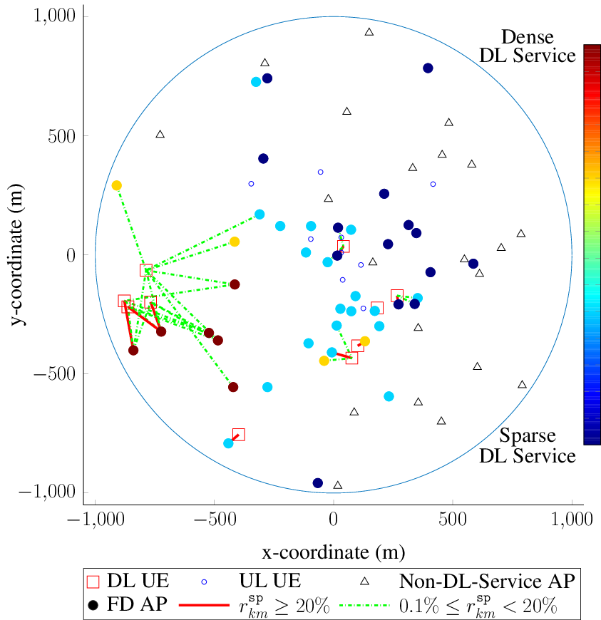
Fig. 4: Service map for DL transmission, where the strong AP-DL UE connections are distinguished by rk​m𝚜𝚙r_{km}^{\mathtt{sp}} (known as r𝚜𝚙(𝐰k​m∗,𝐡^k​m𝚍|𝐰k∗,𝐡^k𝚍)r_{\mathtt{sp}}\bigl(\mathbf{w}_{km}^{*},\mathbf{\hat{h}}_{km}^{\mathtt{d}}|\mathbf{w}_{k}^{*},\mathbf{\hat{h}}_{k}^{\mathtt{d}}\bigr) in (15) for short), with K=L=10K=L=10 and ϖ=10−3/M≈0.002%\varpi=10^{-3}/M\approx 0.002\%.

Differently from UL transmission where the APs passively receive the signals from UL UEs, in DL transmission, the CPU computes the AP-DL UE associations to decide which APs would serve DL UEs. To deeply obtain insights into the proposed algorithm, Fig. 4 presents the service map for DL UEs. In this figure, the DL service density of an AP (on the color bar) is determined by the number of DL UEs served by that AP. Fig. 4 also indicates the significant connections between APs and DL UEs as given by r𝚜𝚙(𝐰k​m∗,𝐡^k​m𝚍|𝐰k∗,𝐡^k𝚍)r_{\mathtt{sp}}\bigl(\mathbf{w}_{km}^{*},\mathbf{\hat{h}}_{km}^{\mathtt{d}}|\mathbf{w}_{k}^{*},\mathbf{\hat{h}}_{k}^{\mathtt{d}}\bigr) in (15). It can be seen that the strong connections are dynamically established among APs and DL UEs in close distances (or with good channel conditions). This phenomenon further verifies the selection of favorable channels discussed in Section IV-B.

VII Conclusion

We have studied an FD CF-mMIMO network, where power control and AP-UE association are jointly optimized under channel uncertainty. First, we have proposed a novel and low-complexity pilot assignment algorithm based on the heap structure to improve the quality of channel estimates. Then, we have introduced the generalized robust design taking into account the CSI errors. The special relationship between binary and continuous variables has been exploited to devise the optimal solution for the ZF-based robust problem. Numerical results have demonstrated that our proposed algorithms outperform the existing robust designs. The effectiveness in handling the AP-DL UE associations has been also verified by a service map.

References

  • [1] A. Yadav et al., “Full-duplex communications: Performance in ultradense mm-wave small-cell wireless networks,” IEEE Veh. Technol. Mag., vol. 13, no. 2, pp. 40–47, June 2018.
  • [2] S. K. Sharma, T. E. Bogale, L. B. Le, S. Chatzinotas, X. Wang, and B. Ottersten, “Dynamic spectrum sharing in 5G wireless networks with full-duplex technology: Recent advances and research challenges,” IEEE Commun. Surveys Tutor., vol. 20, no. 1, pp. 674–707, Firstquarter 2018.
  • [3] A. Sabharwal et al., “In-band full-duplex wireless: Challenges and opportunities,” IEEE J. Select. Areas Commun., vol. 32, no. 9, pp. 1637–1652, Feb. 2014.
  • [4] S. Goyal, P. Liu, S. S. Panwar, R. A. Difazio, R. Yang, and E. Bala, “Full duplex cellular systems: Will doubling interference prevent doubling capacity?” IEEE Commun. Mag., vol. 53, no. 5, pp. 121–127, May 2015.
  • [5] D. Bharadia and S. Katti, “Full duplex MIMO radios,” in Proc. 11th USENIX Symp. Netw. Syst. Design Implement. (NSDI), Seattle, WA, USA, 2014, pp. 369–372.
  • [6] A. Yadav et al., “Energy and traffic aware full duplex communications for 5G systems,” IEEE Access, vol. 5, pp. 11 278–11 290, May 2017.
  • [7] V.-D. Nguyen et al., “Spectral efficiency of full-duplex multiuser system: Beamforming design, user grouping, and time allocation,” IEEE Access, vol. 5, pp. 5785–5797, Mar. 2017.
  • [8] H. V. Nguyen et al., “Joint antenna array mode selection and user assignment for full-duplex MU-MISO systems,” IEEE Trans. Wireless Commun., vol. 18, no. 6, pp. 2946–2963, June 2019.
  • [9] H. V. Nguyen et al., “Joint power control and user association for NOMA-based full-duplex systems,” IEEE Trans. Commun., July 2019, accepted for publication.
  • [10] V.-D. Nguyen, H. V. Nguyen, O. A. Dobre, and O.-S. Shin, “A new design paradigm for secure full-duplex multiuser systems,” IEEE J. Select. Areas Commun., vol. 36, no. 7, pp. 1480–1498, July 2018.
  • [11] H. Q. Ngo et al., “Cell-free massive MIMO versus small cells,” IEEE Trans. Wireless Commun., vol. 16, no. 3, pp. 1834–1850, Mar. 2017.
  • [12] M. Bashar, K. Cumanan, A. G. Burr, M. Debbah, and H. Q. Ngo, “On the uplink max–min SINR of cell-free massive MIMO systems,” IEEE Trans. Wireless Commun., vol. 18, no. 4, pp. 2021–2036, Apr. 2019.
  • [13] T. T. Vu et al., “Full-duplex cell-free massive MIMO,” in Proc. IEEE Inter. Conf. Commun. (ICC), May 2019, pp. 1–6.
  • [14] D. Wang et al., “Performance of network-assisted full-duplex for cell-free massive MIMO,” May 2019. [Online]. Available: http://arxiv.org/abs/1905.11107
  • [15] M. Duarte, C. Dick, and A. Sabharwal, “Experiment-driven characterization of full-duplex wireless systems,” IEEE Trans. Wireless Commun., vol. 11, no. 12, pp. 4296–4307, Dec. 2012.
  • [16] H. V. Nguyen et al., “On the spectral and energy efficiencies of full-duplex cell-free massive MIMO,” Sept. 2019. [Online]. Available: https://arxiv.org/abs/1910.01294
  • [17] T. H. Cormen, C. E. Leiserson, R. L. Rivest, and C. Stein, Introduction to Algorithms, 2nd ed. Cambridge, MA, USA: MIT Press, 2001.
  • [18] D. Korpi, M. Heino, C. Icheln, K. Haneda, and M. Valkama, “Compact inband full-duplex relays with beyond 100 dB self-interference suppression: Enabling techniques and field measurements,” IEEE Trans. Antennas Propagation, vol. 65, no. 2, pp. 960–965, Feb. 2017.