Many-body localization of bosons in optical lattice:
Dynamics in disorder-free potentials
Abstract
The phenomenon of Many-Body Stark Localization of bosons in tilted optical lattice is studied. Despite the fact that no disorder is necessary for Stark localization to occur, it is very similar to well known many body localization (MBL) in sufficiently strong disorder. Not only the mean gap ratio reaches poissonian value as characteristic for localized situations but also the eigenstates reveal multifractal character as in standard MBL. Stark localization enables a coexistence of spacially separated thermal and localized phases in the harmonic trap similarly to fermions. Stark localization may also lead to spectacular trapping of particles in a reversed harmonic field which naively might be considered as an unstable configuration.
I Introduction
Nature seems not to like boredom. When Fermi, Pasta and Ulam wanted to test an approach to ergodicity in nonlinear systems, they found with M. Tsingou, in a famous numerical experiment on coupled nonlinear oscillators, a quasiperiodic motion with energy shared among few modes only (see e.g. Ford 1992). The strongly chaotic classically motion leads to spectra with statistical properties well described by random matrix theory Haake 2010 as revealed e.g. by hydrogen atom in a uniform magnetic field. Yet, a closer both experimental and theoretical analysis revealed system specific regularities traced back to classical periodic orbits (for a review see Friedrich and Wintgen 1989) and semiclassical quantization schemes based on them Gutzwiller 1971 received a deserved verification. Similarly it was believed for a long time that generic many-body systems in their time evolution are faithful to Eigenstate Thermalization Hypothesis (ETH) Deutsch 1991; Srednicki 1994; D’Alessio et al. 2016 with notable exceptions of integrable systems which can be described by generalized Gibbs ensemble – see e.g. Cassidy et al. 2011; Rigol and Srednicki 2012. In one sentence, under ETH few-body observables are expected to thermalize due to interactions within the whole system. A powerful counterexample was found for strongly disordered systems Gornyi et al. 2005; Basko et al. 2006 which was later coined many-body localization (MBL). MBL, a robust ergodicity breaking phenomenon, has been intensively studies since then (for reviews see Huse et al. 2014; Nandkishore and Huse 2015; Alet and Laflorencie 2018; Abanin et al. 2019a). Theoretical studies mainly concentrated on interacting spin systems but experimental demonstration of MBL came with cold atom platforms Schreiber et al. 2015; Lüschen et al. 2017; Lukin et al. 2019; Rispoli et al. 2019. While experiments deal with finite systems, very recently questions about the very existence of MBL in the thermodynamic limit have been posed Šuntajs et al. 2019 initiating a vivid discussion Abanin et al. 2019b; Sierant et al. 2020a; Panda et al. 2020; Šuntajs et al. 2020; Laflorencie et al. 2020; Sierant et al. 2020b. Significant progress has been made in addressing dynamics of large systems Zakrzewski and Delande 2018; Goto and Danshita 2019; Doggen and Mirlin 2019; Chanda et al. 2020a; Chanda et al. 2020b. In here we shall limit ourselves mostly, however, to small systems in the spirit of recent experiments with bosons Lukin et al. 2019; Rispoli et al. 2019 for which simulations may be performed numerically exactly Yao and Zakrzewski 2020. Only for slowly varying harmonic potential we consider larger system sizes using matrix product states formalism Schollwoeck 2011.
MBL is not the only ergodicity breaking mechanism identified recently. Interacting Rydberg atom arrays revealed persistent oscillations Turner et al. 2018; Ho et al. 2019; Khemani et al. 2019; Iadecola and Žnidarič 2019; Schecter and Iadecola 2019 sometimes referred to as quantum scars. However, in traditional quantum chaos language quantum scars denote partial wavefunction localization on unstable periodic orbits Heller 1984; Bogomolny 1988 - as revealed by the mentioned above hydrogen atom in magnetic field problem. The oscillations observed for Rydberg atoms does not seem to have any classical counterpart (see e.g. Mark et al. 2020; Michailidis et al. 2020; Turner et al. 2020). Similarly nonergodic behavior has been observed for models with global constrains, notably lattice gauge theory models Smith et al. 2017; Brenes et al. 2018; Magnifico et al. 2020; James et al. 2019; Chanda et al. 2020c; Giudici et al. 2020; Surace et al. 2020; Feldmeier et al. 2020 or for fragmented Hilbert space Sala et al. 2020; Khemani and Nandkishore 2019; Rakovszky et al. 2020. Recently, strong nonergodic behavior has been predicted for a static uniform force acting on atoms in an optical lattice Schulz et al. 2019; van Nieuwenburg et al. 2019; Taylor et al. 2020. The phenomenon has been naturally called a many-body Stark Localization and has been recently discussed in spinless and spinful fermions Schulz et al. 2019; van Nieuwenburg et al. 2019; Chanda et al. 2020d. The same mechanism has been found to be responsible for the predicted spacial coexistence of extended and localized regions Chanda et al. 2020d. While many-body Stark localization has been considered for spins and fermions, for bosons it was mentioned briefly only Taylor et al. 2020, the aim of this paper is to fill this gap.
MBL of bosons in disordered potential was addressed in several works Aleiner et al. 2010a; Aleiner et al. 2010b; Michal et al. 2016. In optical lattice it shows characteristic features related to the fact that there is no limitation for number of particles occupying a single site. Thus one may expect additional effects due to bunching as, e.g., the existence of the inverse mobility edge, with higher lying states being easier to localized for sufficiently strong interactions Sierant et al. 2017; Sierant and Zakrzewski 2018; Hopjan and Heidrich-Meisner 2020; Yao and Zakrzewski 2020. Also random interactions Sierant et al. 2017 as well as cavity-mediated long-range interactions Sierant et al. 2019a were considered in the context of bosonic MBL. In this paper, we address quantitatively the many-body Stark localization for bosons in the absence of disorder assuming a tilted optical lattice within the standard Bose-Hubbard model. In Section II we demonstrate the existence of localized phase and determine the critical field strengths for the crossover at finite system sizes considered. We analyse also the properties of eigenstates finding them to be multifractal. This property is shared with standard MBL Macé et al. 2019 as well as with ground state features Lindinger et al. 2019 of the model. Later, we consider effects due to an additional harmonic, slowly varying potential on top of the optical lattice that allows us to study the coexistence of both thermal and localized phases in similarity to fermions Chanda et al. 2020d.Finally we show that the fact that the curvature of external potential could suppress transport may lead to the possibility that atoms might be trapped by a reversed harmonic field.
II The Hamiltonian and its spectral properties
We shall consider bosons confined in a quasi one-dimensional optical lattice. We describe the model by a standard Bose-Hubbard Hamiltonian:
| (1) |
where denote bosonic annihilator (creator) operators obeying commutation relation and . For standard MBL studies Sierant and Zakrzewski 2018 one assumes to be random. Instead we shall consider the system in a tilted lattice with the on-site chemical potential of the form of which corresponds to a uniform force acting on bosons. From now on we assume (with being thus a unit of energy). We consider small system sizes with number of sites of the order of inspired by recent experiments Lukin et al. 2019; Rispoli et al. 2019.
It has been found recently Schulz et al. 2019; van Nieuwenburg et al. 2019 that a uniform tilt of the lattice (corresponding to an action of the static electric field) may lead, for spinless fermions, to disorder free localization called many-body Stark localization (MBSL) for a sufficiently large electric field, . Soon the corresponding effect has been addressed with experimentally much easier to realize spinful fermions in the tilted lattice case Kohlert et al. 2020; Chanda et al. 2020d. We shall consider it here for bosons where no additional restrictions due to Pauli exclusion principle are present. As for fermions, MBSL may be viewed as a generalization of Wannier-Stark localization Emin and Hart 1987; Glueck et al. 2002 to the interacting case.

We shall consider mainly the repulsive interactions, . One might expect that for attractive interactions () bosons will tent to group together. This intuition is valid for very low lying energy states, however, we are interested in the properties of highly excited states in the regime of high density of states. Recall that, for , the change of the sign of corresponds to an effective change of the sign of the Hamiltonian (and all the eigenvalues) ) as the sign in front of may be simultaneously changed by the gauge transformation . The same property holds in the presence of . Due to the total particle number conservation the chemical potential term may be made symmetric around the center of the chain and the change of may be accompanied with the chain reflection around the chain centre. Thus spectra of for given values are the same for and . This is an exact symmetry between two Hamiltonians with changed sign and reversed energy ordering of eigenvalues and eigenvectors.
With this said, let us consider first the spectral properties: eigenvalues and eigenvectors of the model (1) with tilt. While in Ref.Schulz et al. 2019 a small harmonic potential is added to a pure linear tilt, we shall follow van Nieuwenburg et al. 2019 and modify the chemical potential adding a small disorder. In effect, we assume in this section
| (2) |
where are random, drawn from a uniform distribution on interval. We take which is sufficiently small that in the absence of the tilt, , the statistics is faithful to Gaussian orthogonal ensemble (GOE) of random matrices Yao and Zakrzewski 2020 for parameters considered. We assume some non-zero disorder to be able to increase statistically the sample of eigenenergies we consider. Typically we consider 200 disorder realizations.
As a simple indicator of the transition between thermal and localized phases, the mean gap ratio is often used Oganesyan and Huse 2007; Luitz et al. 2015; Mondaini and Rigol 2015; Sierant et al. 2019b. It is an average of dimensionless gap ratios defined as
| (3) |
with being the level spacing. Importantly (and thus ) is dimensionless and the tricky procedure of level unfolding Gómez et al. 2002 is not necessary. On the ergodic side as appropriate for Gaussian orthogonal ensemble (GOE) of random matrices while for Poisson statistics (PS) describing the localized case Atas et al. 2013. Fig. 1 shows the mean gap ratio as a function of the lattice tilt (electric field) for different scaled energies of the system for bosons on sites. Following the seminal treatment of MBL in Heisenberg chain Luitz et al. 2015 we define the dimensionless energy to characterize the system. Disorder averaging allows us to get a decent statistics for 20 bins along axis. Left top panel corresponds to small repulsive interaction . Observe that for small the system is delocalized, with close to GOE value (except at the very top energy). For larger , decreases in an energy dependent manner where the energies close to the middle of the spectrum are most resistant to effect of (in the region of largest density of states). Gradually the crossover to a fully localized phase is accomplished around . Note that the critical region of the transition from GOE-like to Poisson-like values is quite broad as might be expected for a small system size considered.
The picture is markedly different for where states for scaled energies show localized character for all values. This is related to the splitting of the Hilbert space into subbands for large interactions Carleo et al. 2012; Sierant and Zakrzewski 2018 - this large in scaled energy region corresponds to a small number of states (very low density). Interesting physics concentrates for low where a strong energy dependence of the localization transition occurs (the situation resembles the mobility edge picture studied for a random disorder in Sierant and Zakrzewski 2018; Yao and Zakrzewski 2020). The transition to a fully localized phase is completed about .
The bottom panels shows the data for the attractive interactions cases, demonstrating that the spectrum is simply reversed with respect to situation, as expected on the symmetry consideration grounds mentioned above. For that reason we discuss the properties of eigenstates for repulsive interactions only.

The dependence of mean gap ratio on energy and control parameter () closely resembles the behavior observed for the crossover to MBL for bosons Yao and Zakrzewski 2020 and spins Luitz et al. 2015 alike. One can pose a question - is it just a similarity of statistical properties of eigenvalues or the eigenstates also share similar properties ? For the disordered Heisenberg chain a detailed study Macé et al. 2019 revealed multifractality of eigenstates across the critical region as well as in the “localized” regime where takes the poissonian value. Let us inspect the properties of eigenstates in the bosonic system. We consider the random on-site disorder case at changing the disorder amplitude in (2)) (such an analysis for bosons is not available till now) and compare it with Stark-localization when changing (with small background disorder ). As in Macé et al. 2019 we consider participation entropies (PE) of eigenstates, of order q defined as:
| (4) |
being an analysed wavefuction. depends of course on the basis chosen, we restrict to the natural Fock basis below. We consider changes of with the system size considering to . In a perfect, GOE like scenario where is the dimension of the Hilbert space. on the other hand, for perfectly localized situation should be size independent. In the transition regime one expects PEs to behave like with the fractal dimension . We call eigenstates multifractal if ’s are different for different Macé et al. 2019.
Fig. 2 presents the results of fitting dependence to the data obtained in both studied cases. Data are averaged, as indicated by the overbar, over 1000 disorder realizations except for case with 192 realizations. Typically we take up to 200 eigenstates corresponding to energies around except for smaller values where necessarily this number is much smaller. For when we take just five eigenvalues per realization. Still the error bars obtained for the average entropies are of the order of symbols sizes. While the system sizes studied are much smaller than for the spin-1/2 Heisenberg case, we observe a striking similarity to the results presented in Macé et al. 2019. It is probably less surprizing that bosons in random disorder reveal a similar trend as spins - after all it is a common believe that general features of MBL phase are similar for different systems. However, a similarity between the disorder driven (top row) and the electric field driven (bottom row) behavior of apparent from Fig. 2 is really striking.
The fitted parameters for sites are collected in Fig. 3. We observe that and are different from each other for both disorder driven and electric field driven models – the eigenstates are multifractal even in the regime considered as localized. Moreover, we observe that the free term changes the sign from negative to positive values with increasing disorder (top panel) - a feature also observed for the Heisenberg spin chain Macé et al. 2019. The change of sign of has been identified in Macé et al. 2019 as an indicator of the critical disorder value for the transition. In our case changes the sign around – compare Fig. 3 – while the transition to MBL occurs, according to -statistics, for Yao and Zakrzewski 2020 around i.e. the value around which we collect for analysis. While this discrepancy is quite significant, let us note large error bars on coefficients resulting from the fits, so this discrepancy is within the bounds given by those error bars. Interestingly, the error bars on dimensionality are much smaller and practically within the size of markers in Fig. 3.

The bottom row in Fig. 3 analyses the dependence for the tilted lattice. As for spacings analysis, we add a tiny disorder with amplitude to enable averaging over the disorder realizations. Similarly to the random disorder case, we observe a gradual change of slopes of the fits with increasing tilt, , of the lattice. Even for the largest values of the multifractal properties of eigenstates persists. Overall the similarity of these two cases of disordered and tilted lattice suggests that MBL and MBSL are very closely related. An interesting behaviour is revealed in the fitted coefficients dependence on which is not monotonic, in contrast to the random case. One observes a fast growth of for small with the maximum around and a subsequent decrease. Only for much larger a “standard”’ change of the sign occurs. This behaviour may be related to the fact that the hopping between neighboring sites becomes quasi-resonant around as the additional energy may be supplied by the interaction energy in the case studied. These values of lead to an enhanced transport in the time dynamics as we shall show below. One should, however, keep in mind a relative large error of coefficients in this regime.
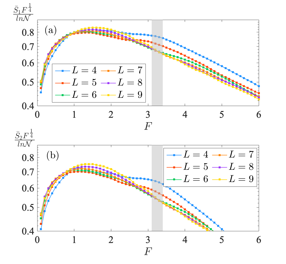
Rescaling the participation entropies by the logarithm of the Hilbert space dimension (again we precisely follow the scaling analysis of the participation entropy advanced in Macé et al. 2019 for the case of spin models) we may observe a crossing of curves representing for different system sizes - see Fig. 4. Multiplication of the data by factor does not affect the size-dependent crossings but helps enhancing the details of the crossing. Both the and the data cross for except the data for the smallest system sizes that we disregard. In this way the critical field value, , corresponding to the onset of localized regime may be identified.
III Transport and Localization


While spectral properties characterise the system in quite a complete way, in view of possible experiments we address the time dynamics in the system. For small number of sites in bosonic system it was shown Rispoli et al. 2019 that a complete characterization of occupation of sites and their correlations is accessible. With these impressive results in mind we consider the time dynamics for an unit average filling per site. Using Chebyshev propagation scheme Tal-Ezer and Kosloff 1984; Leforestier et al. 1991; Fehske et al. 2009 we can reach sites with bosons, the system not easily accessible for direct diagonalization. As the initial stare we consider an uniformly filled Fock state with one particle at each site: state, then observe its time evolution in a tilted lattice. We collect the final occupation pattern around for as shown in Fig. 5. For the initially symmetric in space state remains symmetric with nearly uniform occupations except at the edges (we consider open boundary conditions), as we know from earlier studies Yao and Zakrzewski 2020 the state becomes significantly entangled during time evolution. The spacial symmetry is broken for non-zero . Small values lead to transport of bosons which accumulate at one side due to the tilt of the optical lattice. This behaviour is reversed for larger values, when the localization sets in and the almost uniform occupation of sites is observed even after a long time – see Fig. 5(b) for . For stronger interactions , Fig. 5(c), one could naively expect that bosons repel stronger and the uniform site distribution is created for smaller . This is not the case, we see that even for the strongest considered value a slight asymmetry remains close to the edges of the system - it correlates well with the gap ratio behavior in Fig. 1 where, for strong interaction case the border of MBSL is shifted to .
The attractive interaction case – Fig. 5(d-e) is pretty interesting. Contrary to the intuition the bosons, outside of the localization regime, move against the potential and accumulate at high potential energy end. The picture is just a mirror image of the behavior due to the symmetries of the Hamiltonian discussed above.
To quantify the degree of net transport induced by the tilt we define the Accumulation Factor (AF) as:
| (5) |
so that measures a fraction of particles occupying the left hand half chain with corresponding to the same mean occupation of left and right half chain. This is the case for as well as when a strong MBSL sets in. can be measured at arbitrary , we present its dependence at the exemplary final time for all four different cases considered in Fig. 5(f). For positive both curves reveal an initial growth and then the decay when MBSL sets in. For around comes back entirely to 0.5 value - this correlates again very well the the gap ratio statistics. For apparently MBSL is not complete even at .
To analize the transition to MBSL by time dynamics, we plot in Fig. 5 for (g) and (h), respectively. For bosons on sites we follow the time dependence of up to , respectively in the logarithmic scale. The values taken are below full MBSL case and one may clearly identify three regimes: (i) a fast initial redistribution of particles on the time scale of few tunneling times; (ii) almost linear growth (on the logarithmic scale) corresponding to slow subdiffusive-like growth (iii) saturation when the quasi-stationary distribution is reached (for small system sizes considered). This behavior of resembles to a large extend the time dynamics of the transport distance analysed in the transition to MBL in Rispoli et al. 2019; Yao and Zakrzewski 2020. The latter quantity requires two-point correlation function evaluation while relies on occupations only.
Observe that the data for larger values, corresponding to localization with low appear more noisy in Fig. 5. This is due to the fact that apparently few eigenstates contribute significantly to the evolution of the initial wavepacket resulting in the quasiperiodic oscillation of observables. Such oscillations look quite irregular on a logarithmic scale.

It has been noted Schulz et al. 2019; Taylor et al. 2020 that the system in tilted lattice belongs to a class of systems with global constrains, not only the charge (the particle number) but also the dipole moment is conserved. For such systems fracton excitations are claimed to be responsible for eventual thermalization of the system at very long time due to very slow dynamic of hydrodynamical origin Feldmeier et al. 2020; Gromov et al. 2020. To overcome these effects and observe truly localized systems additional small terms to the Hamiltonian are added as a small disorder van Nieuwenburg et al. 2019 or a small additional harmonic potential at sites adding to in (2) the additional term . While such an approach is necessary for level spacing analysis (due to quasi-degeneracies in the spectrum for pure Stark problem Schulz et al. 2019; Taylor et al. 2020) the fracton dynamics does not occur on the experimental time scale as shown by comparison of the dynamics with and without the additional harmonic term – Fig. 6.
IV Bosons in a tight harmonic trap
The harmonic trap in some form typically accompanies the optical lattice potential. Typically in experiments the curvature of the potential is quite tiny, promising that systems to be studied are locally uniform. Even then it may lead to coexistence of different phases as exemplified by the famous cake shape for the ground state occupation of bosons within Bose-Hubbard model where a harmonic potential modifies local chemical potential creating regions of Mott insulator and superfluid phases (for a review see Bloch et al. 2008). By shaping light with digital micromirror devices Gauthier et al. 2016; Mazurenko et al. 2017 or spatial light modulators Gaunt 2015 one can remove the undesired remaining trapping potentials or add an arbitrarily designed envelope to the system studied. Modifying the curvature one may improve adiabatic loading of cold atoms into the ground state Rey et al. 2006; Zakrzewski and Delande 2009 and have access to the compressibility of the sample Delande and Zakrzewski 2009.
Recently the dynamics of excited states in the presence of a harmonic trap on top of the optical lattice potential has also been studied. It was demonstrated that extended and localized phases may coexist for spinless as well as spinful fermions Chanda et al. 2020d. Hereby, we test the same idea for bosons assuming the chemical potential in the form.
| (6) |
where is the center of the trap.

We visualize the coexistence phenomenon induced by harmonic trap by considering the time evolution of a staggered initial state in a chain with 64 sites. To treat such a relatively large system at half filling we use time dependent variational principle (TDVP) algorithm(for a review of numerical tools enabling study of time dynamics for large system sizes see Paeckel et al. 2019). In the simulation we assume maximal number of bosons per site, using typically auxilliary space dimension and . The simulation is performed with time step and cut-off . Tests of convergence show that the results are reliable for times considered in later discussion. At sufficient long time, the middle of chain appears to be thermalizing and the initial staggered occupations spread over the central region - compare Fig. 7. However, in both outer regions the system preserves the memory of its original configuration showing the lack of thermalization - localization occurs. By increasing the curvature , the boundary separating the apparently coexisting localized and thermalized regions moves towards the center.
As observed by us for fermions Chanda et al. 2020d an understanding of this behavior may be obtained invoking the notion of the local field . If the local field in a given region is sufficiently strong so it would lead to localization in a tilted lattice, one may expect localization in this region (of sufficiently large curvature). For fermions, there is a strict correspondence between the critical field leading to localization and the local field leading to a separation of delocalized center of the trap from the localized sides for which . The same approach, using the critical field obtained previously (compare Fig. 4), yields dashed lines estimates that are close to the boundary of two phases, supporting our local field hypothesis. The central delocalized region exceeds a little the local field borders for .
For (Fig. 7(c)) there is an unexpected pattern in time evolution: an excitation emerges from the center, penetrates the localized region moving outwards with a small spread. This resonance-like effect may be understood (we are grateful to Piotr Sierant for contributing his insight to this point) considering the family of states that, for are degenerate with the initial state :
| (7) | ||||
as the energy difference between state and state is . Within this degenerate subspace is coupled to by a two-fold action of the hopping term, i.e.boson on site hops onto site and boson from hops onto . The two processes sum up to a second order process occuring at a position-depending rate
| (8) | ||||
where, recall, is the trap center. To simplify the argument let us count the index from the center of the trap, effectively shifting . We get then the decreasing series of effective hopping rates forming a series of time scales for entangling with . Since is nothing as a discretized distance from the center of the trap, we have a parabolic dependence linking time with distance . Such a parabola is indeed observed in Fig. 7(c). The resonance occurs for arbitrary once condition is satisfied as shown in Fig. 8.

Observe that the prominent “parabola” excitation, described above, is followed for , by additional emissions creating small local grains of roughly half-integer populations. Those grains seem to lay on another parabola’s with a slower spread. We believe that they are due to higher order processes within the discussed degenerate manifold.
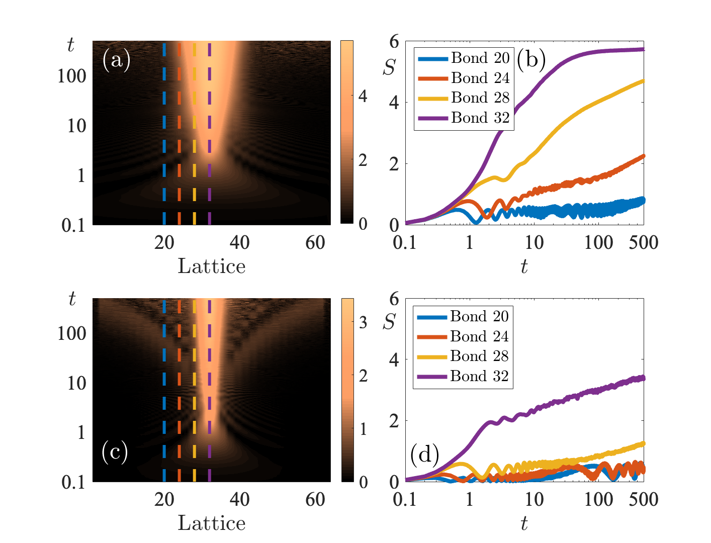
The entanglement entropy growth follows the occupations pattern, again in a close similarity with the fermionic case Chanda et al. 2020d. In the central delocalizing region the entropy (as measured on different bonds) grows rapidly and saturates, while in the localized outer regions it exhibits logarithmic growth as in SMBL case - compare Fig. 9. A closer inspection of Fig. 7 and the upper row of Fig. 9 shows interesting feature. While occupations redistribute themselves very fast and the occupations practically equalize in the central region on the time scale of few tunneling times, the entanglement entropy shows a different behavior. It grows fast for the central bond but the growth is much slower at bonds say 28 and 24 which are within the thermalizing region. In effect, the region of large entropy spreads slowly in time, staying well within the borders given by the local field estimate. Such a slow down of the growth of the entanglement entropy inside the thermalizing center was observed already for fermions Chanda et al. 2020d. It was attributed to the fact that due to small local Hilbert space for fermions there are limitations on the difference between entanglement entropies on nearby bonds. Thus a slow growth on the localized side affects also the growth in the central region. Interestingly we observe the same behavior for bosons for which, in principle, the dimension of the local Hilbert space is unlimited (it is limited in our calculations to but we have checked that the increase of does not affect the time dynamics of entropy).
For the resonance case, the emission effects are visible also in the entropy growth - we observe an oscillatory dynamics imposed on the growth. peaks when the excitation propagates across the bond to be considered, and the subsequent emissions lead, similarly, to additional oscillations.
To end this section we present the evidence for the convergence of our simulations by considering the entanglement entropy at different bonds for different auxiliary space dimension . We investigate and extract from the same bonds as in Fig. 9. The weaker the harmonic trap is, the larger is required for a given accuracy (the thermalizing central region is bigger). Therefore, we show and cases – see Fig. 10. For , provides a satisfactory convergence for all bonds up to , while for even such a large value is insufficient for the central bond. Observe that the convergence is restored quite fast when moving away from the very center of the trap, even well within the thermalizing center. Since we do not analyse in detail properties of the system in the very center of the trap a simulation with is already a good choice for or larger while for is definitely required. As it is clear from lower panels in Fig. 9 also in the resonant case, despite travelling excitations, the entropy growth is limited and may be reliably simulated with .

V Inverted trap and its confinement
We have observed that the harmonic potential on top of the optical lattice could induce coexistence of localized and thermal phases strongly suppressing the transport between these domains. The effect is due to local effective electric fields that, if exceeding the threshold value, lead to localization. The effect does not depend on the sign of the curvature, as what really matters is the local field. In effect, an inverse harmonic trap should also be able to prevent atoms from expansion and loss. The effect is entirely of different origin from the fact that, a long-lived attractively interacting bosons may be confined in inverse trap as demonstrated by Braun et al. 2013 as a consequence of negative temperature. In our case the confinement is due to localization induced suppresion of transport and is independent (or weakly dependent) on the sign of the interaction.
Let us demonstrate the effect in a chain of size and consider as the initial state a pure state with middle 14 sites occupied by one particle each with the rest of the chain being empty. This configuration is, with no doubt, unstable and all particles should expand with repulsive interaction while shrinking for sufficiently large . The simulation could be considered as a simplified version for an expansion of initially well-confined atomic gas. For attractive interactions , the occupations evolved with time under reversed trap are depicted in the top row of Fig. 11. The atoms accumulate in the center - the simulation reflects simply earlier experimental results Braun et al. 2013, indicating a long-lived trapped mode interpretted as the negative temperature effect. However, for , while intuitively the gas should expand across the lattice, the expansion is stopped when the local field reaches critical value. Atoms are “forbidden” to enter the localized regime - the wavepacket has apparently vanishingly small overlap on eigenstates strongly localized in the outer region. As revealed by inspection of Fig. 11, the difference between the interactions being attractive or repulsive shows as the distribution of particles in the central region: for attractive case they tend to occupy the very center forming a is single peak but for the repulsive case there is an excess populations close to the boundaries of the central region.

VI Conclusions
We have shown that interacting bosons in optical lattice may be many-body localized in the presence of a local force in similarity with spinless and spinful fermions. The resulting Stark many-body localization is similar to disorder induced MBL - in particular eigenstates in the localized regime show multifractal properties. The Stark MBL has an impact on the behavior of interacting particles in an arbitrary potential - we demonstrate in detail the system dynamics in the presence of the harmonic trap. Then the coexistence of apparently thermalizing region with outer regions exhibiting strong localization has been demonstrated, in analogy to the similar behavior observed for fermions Chanda et al. 2020d. The border separating localized and thermal parts is, to a good precision, given by the critical value of the static field (force) which leads to Stark many body localized system in the tilted lattice. Such a local field value is given by the spacial derivative of the potential (not necessarily harmonic) so the effect should not be limited to harmonic potential but it is rather a generic feature of slowly varying potentials. As an example we show that even in the inverted harmonic trap which is supposed to loss atoms rapidly – surprisingly no losses appear and the atomic cloud is well confined as a consequence of suppression of transport into the many-body Stark localized neighboring regions. More complicated in shape potentials may separate the space into several regions with transport practically prohibited between them.
Our numerical results are either related to small systems amenable to exact treatment (via diagonalization or Chebyshev propagation) or to typical experimental times of hundreds of tunneling times (for TDVP simulations). This does not preclude that, for example, the coexistence of localized and thermal regions very slowly fades away in the large systems/long times limit. Additional studies are needed to resolve those issues. Such studies are, however, at the border of current numerical capabilities.
Acknowledgements.
We are grateful to Titas Chanda and Piotr Sierant for discussions on different aspects of this work and remarks on the manuscript. The numerical computations have been possible thanks to High-Performance Computing Platform of Peking University. Support of PL-Grid Infrastructure is also acknowledged. The TDVP simulations have been performed using ITensor library (https://itensor.org). This research has been supported by National Science Centre (Poland) under project 2019/35/B/ST2/00034 (J.Z.).References
- Ford (1992) J. Ford, Physics Reports 213, 271 (1992).
- Haake (2010) F. Haake, Quantum Signatures of Chaos (Springer, Berlin, 2010).
- Friedrich and Wintgen (1989) H. Friedrich and H. Wintgen, Physics Reports 183, 37 (1989).
- Gutzwiller (1971) M. C. Gutzwiller, Journal of Mathematical Physics 12, 343 (1971).
- Deutsch (1991) J. M. Deutsch, Phys. Rev. A 43, 2046 (1991).
- Srednicki (1994) M. Srednicki, Phys. Rev. E 50, 888 (1994).
- D’Alessio et al. (2016) L. D’Alessio, Y. Kafri, A. Polkovnikov, and M. Rigol, Advances in Physics 65, 239 (2016), https://doi.org/10.1080/00018732.2016.1198134 .
- Cassidy et al. (2011) A. C. Cassidy, C. W. Clark, and M. Rigol, Physical Review Letters 106 (2011), 10.1103/physrevlett.106.140405.
- Rigol and Srednicki (2012) M. Rigol and M. Srednicki, Physical Review Letters 108 (2012), 10.1103/physrevlett.108.110601.
- Gornyi et al. (2005) I. V. Gornyi, A. D. Mirlin, and D. G. Polyakov, Phys. Rev. Lett. 95, 206603 (2005).
- Basko et al. (2006) D. Basko, I. Aleiner, and B. Altschuler, Ann. Phys. (NY) 321, 1126 (2006).
- Huse et al. (2014) D. A. Huse, R. Nandkishore, and V. Oganesyan, Phys. Rev. B 90, 174202 (2014).
- Nandkishore and Huse (2015) R. Nandkishore and D. A. Huse, Annual Review of Condensed Matter Physics 6, 15 (2015).
- Alet and Laflorencie (2018) F. Alet and N. Laflorencie, Comptes Rendus Physique 19, 498 (2018).
- Abanin et al. (2019a) D. A. Abanin, E. Altman, I. Bloch, and M. Serbyn, Rev. Mod. Phys. 91, 021001 (2019a).
- Schreiber et al. (2015) M. Schreiber, S. S. Hodgman, P. Bordia, H. P. Lüschen, M. H. Fischer, R. Vosk, E. Altman, U. Schneider, and I. Bloch, Science 349, 842 (2015).
- Lüschen et al. (2017) H. P. Lüschen, P. Bordia, S. Scherg, F. Alet, E. Altman, U. Schneider, and I. Bloch, Phys. Rev. Lett. 119, 260401 (2017).
- Lukin et al. (2019) A. Lukin, M. Rispoli, R. Schittko, M. E. Tai, A. M. Kaufman, S. Choi, V. Khemani, J. Léonard, and M. Greiner, Science 364, 256 (2019).
- Rispoli et al. (2019) M. Rispoli, A. Lukin, R. Schittko, S. Kim, M. E. Tai, J. Léonard, and M. Greiner, Nature 573, 385 (2019).
- Šuntajs et al. (2019) J. Šuntajs, J. Bonča, T. Prosen, and L. Vidmar, (2019), arXiv:1905.06345 .
- Abanin et al. (2019b) D. A. Abanin, J. H. Bardarson, G. D. Tomasi, S. Gopalakrishnan, V. Khemani, S. A. Parameswaran, F. Pollmann, A. C. Potter, M. Serbyn, and R. Vasseur, “Distinguishing localization from chaos: challenges in finite-size systems,” (2019b), arXiv:1911.04501 .
- Sierant et al. (2020a) P. Sierant, D. Delande, and J. Zakrzewski, Phys. Rev. Lett. 124, 186601 (2020a).
- Panda et al. (2020) R. K. Panda, A. Scardicchio, M. Schulz, S. R. Taylor, and M. Žnidarič, Europhysics Letters 128, 67003 (2020).
- Šuntajs et al. (2020) J. Šuntajs, J. Bonča, T. Prosen, and L. Vidmar, arXiv e-prints , arXiv:2004.01719 (2020), arXiv:2004.01719 [cond-mat.dis-nn] .
- Laflorencie et al. (2020) N. Laflorencie, G. Lemarié, and N. Macé, arXiv e-prints , arXiv:2004.02861 (2020), arXiv:2004.02861 [cond-mat.dis-nn] .
- Sierant et al. (2020b) P. Sierant, M. Lewenstein, and J. Zakrzewski, “Polynomially filtered exact diagonalization approach to many-body localization,” (2020b), arXiv:2005.09534 [cond-mat.dis-nn] .
- Zakrzewski and Delande (2018) J. Zakrzewski and D. Delande, Phys. Rev. B 98, 014203 (2018).
- Goto and Danshita (2019) S. Goto and I. Danshita, Phys. Rev. B 99, 054307 (2019).
- Doggen and Mirlin (2019) E. V. H. Doggen and A. D. Mirlin, Phys. Rev. B 100, 104203 (2019).
- Chanda et al. (2020a) T. Chanda, P. Sierant, and J. Zakrzewski, Phys. Rev. B 101, 035148 (2020a).
- Chanda et al. (2020b) T. Chanda, P. Sierant, and J. Zakrzewski, Phys. Rev. Research 2, 032045 (2020b).
- Yao and Zakrzewski (2020) R. Yao and J. Zakrzewski, Phys. Rev. B 102, 014310 (2020).
- Schollwoeck (2011) Schollwoeck, Ann. Phys. (NY) 326, 96 (2011).
- Turner et al. (2018) C. J. Turner, A. A. Michailidis, D. A. Abanin, M. Serbyn, and Z. Papić, Nature Physics 14, 745–749 (2018).
- Ho et al. (2019) W. W. Ho, S. Choi, H. Pichler, and M. D. Lukin, Phys. Rev. Lett. 122, 040603 (2019).
- Khemani et al. (2019) V. Khemani, C. R. Laumann, and A. Chandran, Physical Review B 99, 161101 (2019).
- Iadecola and Žnidarič (2019) T. Iadecola and M. Žnidarič, Phys. Rev. Lett. 123, 036403 (2019).
- Schecter and Iadecola (2019) M. Schecter and T. Iadecola, Phys. Rev. Lett. 123, 147201 (2019).
- Heller (1984) E. J. Heller, Phys. Rev. Lett. 53, 1515 (1984).
- Bogomolny (1988) E. Bogomolny, Physica D 31, 169 (1988).
- Mark et al. (2020) D. K. Mark, C.-J. Lin, and O. I. Motrunich, Phys. Rev. B 101, 195131 (2020).
- Michailidis et al. (2020) A. A. Michailidis, C. J. Turner, Z. Papić, D. A. Abanin, and M. Serbyn, Phys. Rev. Research 2, 022065 (2020).
- Turner et al. (2020) C. J. Turner, J.-Y. Desaules, K. Bull, and Z. Papić, “Correspondence principle for many-body scars in ultracold rydberg atoms,” (2020), arXiv:2006.13207 [quant-ph] .
- Smith et al. (2017) A. Smith, J. Knolle, R. Moessner, and D. L. Kovrizhin, Phys. Rev. Lett. 119, 176601 (2017).
- Brenes et al. (2018) M. Brenes, M. Dalmonte, M. Heyl, and A. Scardicchio, Phys. Rev. Lett. 120, 030601 (2018).
- Magnifico et al. (2020) G. Magnifico, M. Dalmonte, P. Facchi, S. Pascazio, F. V. Pepe, and E. Ercolessi, Quantum 4, 281 (2020).
- James et al. (2019) A. J. A. James, R. M. Konik, and N. J. Robinson, Phys. Rev. Lett. 122, 130603 (2019).
- Chanda et al. (2020c) T. Chanda, J. Zakrzewski, M. Lewenstein, and L. Tagliacozzo, Phys. Rev. Lett. 124, 180602 (2020c).
- Giudici et al. (2020) G. Giudici, F. M. Surace, J. E. Ebot, A. Scardicchio, and M. Dalmonte, Phys. Rev. Research 2, 032034 (2020).
- Surace et al. (2020) F. M. Surace, P. P. Mazza, G. Giudici, A. Lerose, A. Gambassi, and M. Dalmonte, Phys. Rev. X 10, 021041 (2020).
- Feldmeier et al. (2020) J. Feldmeier, P. Sala, G. de Tomasi, F. Pollmann, and M. Knap, “Anomalous diffusion in dipole- and higher-moment conserving systems,” (2020), arXiv:2004.00635 [cond-mat.str-el] .
- Sala et al. (2020) P. Sala, T. Rakovszky, R. Verresen, M. Knap, and F. Pollmann, Physical Review X 10 (2020), 10.1103/physrevx.10.011047.
- Khemani and Nandkishore (2019) V. Khemani and R. Nandkishore, “Local constraints can globally shatter hilbert space: a new route to quantum information protection,” (2019), arXiv:1904.04815 .
- Rakovszky et al. (2020) T. Rakovszky, P. Sala, R. Verresen, M. Knap, and F. Pollmann, Physical Review B 101, 125126 (2020).
- Schulz et al. (2019) M. Schulz, C. A. Hooley, R. Moessner, and F. Pollmann, Phys. Rev. Lett. 122, 040606 (2019).
- van Nieuwenburg et al. (2019) E. van Nieuwenburg, Y. Baum, and G. Refael, Proceedings of the National Academy of Sciences 116, 9269 (2019).
- Taylor et al. (2020) S. R. Taylor, M. Schulz, F. Pollmann, and R. Moessner, Phys. Rev. B 102, 054206 (2020).
- Chanda et al. (2020d) T. Chanda, R. Yao, and J. Zakrzewski, Phys. Rev. Research 2, 032039 (2020d).
- Aleiner et al. (2010a) I. L. Aleiner, B. L. Altshuler, and G. V. Shlyapnikov, Nat Phys 6, 900 (2010a).
- Aleiner et al. (2010b) I. L. Aleiner, B. L. Altshuler, and G. V. Shlyapnikov, Nature Physics 6, 900 EP (2010b), article.
- Michal et al. (2016) V. P. Michal, I. L. Aleiner, B. L. Altshuler, and G. V. Shlyapnikov, Proceedings of the National Academy of Sciences 113, E4455 (2016).
- Sierant et al. (2017) P. Sierant, D. Delande, and J. Zakrzewski, Acta Phys. Polon. A 132, 1707 (2017).
- Sierant and Zakrzewski (2018) P. Sierant and J. Zakrzewski, New Journal of Physics 20, 043032 (2018).
- Hopjan and Heidrich-Meisner (2020) M. Hopjan and F. Heidrich-Meisner, Phys. Rev. A 101, 063617 (2020).
- Sierant et al. (2017) P. Sierant, D. Delande, and J. Zakrzewski, Phys. Rev. A 95, 021601 (2017).
- Sierant et al. (2019a) P. Sierant, K. Biedroń, G. Morigi, and J. Zakrzewski, SciPost Phys. 7, 8 (2019a).
- Macé et al. (2019) N. Macé, N. Laflorencie, and F. Alet, SciPost Phys. 6, 50 (2019).
- Lindinger et al. (2019) J. Lindinger, A. Buchleitner, and A. Rodríguez, Phys. Rev. Lett. 122, 106603 (2019).
- Kohlert et al. (2020) T. Kohlert, S. Scherg, B. H. Madhusudhana, I. Bloch, and M. Aidelsburger, Bull. Amer. Phys. Soc. (2020).
- Emin and Hart (1987) D. Emin and C. F. Hart, Phys. Rev. B 36, 7353 (1987).
- Glueck et al. (2002) M. Glueck, R. Kolovsky, Andrey, and H. J. Korsch, Phys. Rep. 366, 103 (2002).
- Oganesyan and Huse (2007) V. Oganesyan and D. A. Huse, Phys. Rev. B 75, 155111 (2007).
- Luitz et al. (2015) D. J. Luitz, N. Laflorencie, and F. Alet, Phys. Rev. B 91, 081103 (2015).
- Mondaini and Rigol (2015) R. Mondaini and M. Rigol, Phys. Rev. A 92, 041601 (2015).
- Sierant et al. (2019b) P. Sierant, A. Maksymov, M. Kuś, and J. Zakrzewski, Phys. Rev. E 99, 050102 (2019b).
- Gómez et al. (2002) J. M. G. Gómez, R. A. Molina, A. Relaño, and J. Retamosa, Phys. Rev. E 66, 036209 (2002).
- Atas et al. (2013) Y. Y. Atas, E. Bogomolny, O. Giraud, and G. Roux, Phys. Rev. Lett. 110, 084101 (2013).
- Carleo et al. (2012) G. Carleo, F. Becca, M. Schiro, and M. Fabrizio, Scientific Reports 2, 243 EP (2012), article.
- Macé et al. (2019) N. Macé, F. Alet, and N. Laflorencie, Phys. Rev. Lett. 123, 180601 (2019).
- Tal-Ezer and Kosloff (1984) H. Tal-Ezer and R. Kosloff, J. Chem. Phys. 81, 3967 (1984).
- Leforestier et al. (1991) C. Leforestier, R. Bisseling, C. Cerjan, M. Feit, R. Friesner, A. Guldberg, A. Hammerich, G. Jolicard, W. Karrlein, H.-D. Meyer, N. Lipkin, O. Roncero, and R. Kosloff, J. Comput. Phys. 94, 59 (1991).
- Fehske et al. (2009) H. Fehske, J. Schleede, G. Schubert, G. Wellein, V. S. Filinov, and A. R. Bishop, Physics Letters A 373, 2182 (2009).
- Gromov et al. (2020) A. Gromov, A. Lucas, and R. M. Nandkishore, Phys. Rev. Research 2, 033124 (2020).
- Bloch et al. (2008) I. Bloch, J. Dalibard, and W. Zwerger, Rev. Mod. Phys. 80, 885 (2008).
- Gauthier et al. (2016) G. Gauthier, I. Lenton, N. M. Parry, M. Baker, M. J. Davis, H. Rubinsztein-Dunlop, and T. W. Neely, Optica 3, 1136 (2016).
- Mazurenko et al. (2017) A. Mazurenko, C. S. Chiu, G. Ji, M. F. Parsons, M. Kanász-Nagy, R. Schmidt, F. Grusdt, E. Demler, D. Greif, and M. Greiner, Nature 545, 462 (2017).
- Gaunt (2015) A. Gaunt, Degenerate Bose Gases: Tuning Interactions & Geometry (University of Cambridge, 2015).
- Rey et al. (2006) A. M. Rey, G. Pupillo, and J. V. Porto, Phys. Rev. A 73, 023608 (2006).
- Zakrzewski and Delande (2009) J. Zakrzewski and D. Delande, Phys. Rev. A 80, 013602 (2009).
- Delande and Zakrzewski (2009) D. Delande and J. Zakrzewski, Phys. Rev. Lett. 102, 085301 (2009).
- Paeckel et al. (2019) S. Paeckel, T. Köhler, A. Swoboda, S. R. Manmana, U. Schollwöck, and C. Hubig, Annals of Physics 411, 167998 (2019).
- Braun et al. (2013) S. Braun, J. P. Ronzheimer, M. Schreiber, S. S. Hodgman, T. Rom, I. Bloch, and U. Schneider, Science 339, 52 (2013), https://science.sciencemag.org/content/339/6115/52.full.pdf .