Graph Convolutional Networks for Graphs
Containing Missing Features
Abstract.
Graph Convolutional Network (GCN) has experienced great success in graph analysis tasks. It works by smoothing the node features across the graph. The current GCN models overwhelmingly assume that the node feature information is complete. However, real-world graph data are often incomplete and containing missing features. Traditionally, people have to estimate and fill in the unknown features based on imputation techniques and then apply GCN. However, the process of feature filling and graph learning are separated, resulting in degraded and unstable performance. This problem becomes more serious when a large number of features are missing. We propose an approach that adapts GCN to graphs containing missing features. In contrast to traditional strategy, our approach integrates the processing of missing features and graph learning within the same neural network architecture. Our idea is to represent the missing data by Gaussian Mixture Model (GMM) and calculate the expected activation of neurons in the first hidden layer of GCN, while keeping the other layers of the network unchanged. This enables us to learn the GMM parameters and network weight parameters in an end-to-end manner. Notably, our approach does not increase the computational complexity of GCN and it is consistent with GCN when the features are complete. We demonstrate through extensive experiments that our approach significantly outperforms the imputation based methods in node classification and link prediction tasks. We show that the performance of our approach for the case with a low level of missing features is even superior to GCN for the case with complete features. †† Corresponding author.
Keywords:
Graph convolutional network, GCN, Missing data, Incomplete data, Graph embedding, Network representation learning1. Introduction
Graphs are used in many branches of science as a way to represent the patterns of connections between the components of complex systems, including social analysis, product recommendation, web search, disease identification, brain function analysis, and many more.
In recent years there is a surge of interest in learning on graph data. Graph embedding (Cui et al. 2018; Wang et al. 2017; Ji et al. 2020) aims to learn low-dimensional vector representations for nodes or edges. The learned representations encode structural and semantic information transcribed from the graph and can be used directly as the features for downstream graph analysis tasks. Representative works on graph embedding include random walk and skip-gram model based methods (Perozzi et al. 2014), matrix factorization based approaches (Qiu et al. 2018; Liu et al. 2019), edge reconstruction based methods (Tang et al. 2015), and deep learning based algorithms (Wang et al. 2016; Pan et al. 2018), etc.
Meanwhile, graph neural network (GNN) (Scarselli et al. 2008; Zhou et al. 2018; Wu et al. 2020), as a type of neural network architectures that can operate on graph structure, has achieved superior performance in graph analysis and shown promise in various applications such as visual question answering (Narasimhan et al. 2018), point clouds classification and segmentation (Simonovsky and Komodakis 2017), fraud detection (Liu et al. 2020), machine translation (Bastings et al. 2017), molecular fingerprints prediction (Duvenaud et al. 2015), protein interface prediction (Fout et al. 2017), topic modeling (Yang et al. 2020), and social recommendation (Ying et al. 2018).
Among various kinds of GNNs, graph convolutional network (GCN) (Kipf and Welling 2017), a simplified version of spectral graph convolutional networks (Shuman et al. 2013), has attracted a large amount of attention. GCN and its subsequent variants can be interpreted as smoothing the node features in the neighborhoods guided by the graph structure, and have experienced great success in graph analysis tasks, such as node classification (Kipf and Welling 2017), graph classification (Zhang et al. 2018), link prediction (Kipf and Welling 2016), graph similarity estimation (Bai et al. 2019), node ranking (Maurya et al. 2019; Chen et al. 2019), and community detection (Jin et al. 2019; Choong et al. 2018).

The current GCN-like models assume that the node feature information is complete. However, real-world graph data are often incomplete and containing missing node features. Much of the missing features arise from the following sources. First, some features can be missing because of mechanical/electronic failures or human errors during the data collection process. Secondly, it can be prohibitively expensive or even impossible to collect the complete data due to its large size. For example, social media companies such as Twitter and Facebook have restricted the crawlers to collect the whole data. Thirdly, we cannot obtain sensitive personal information. In a social network, many users are unwilling to provide information such as address, nationality, and age to protect personal privacy. Finally, graphs are dynamic in nature, and thus newly joined nodes often have very little information. All these aspects result in graphs containing missing features.
To deal with the above problem, the traditional strategy is to estimate and fill in the unknown values before applying GCN. For this purpose, people have proposed imputation techniques such as mean imputation (García-Laencina et al. 2010; Yi et al. 2020), soft imputation based on singular value decomposition (Mazumder et al. 2010), and machine learning methods such as k-NN model (Batista et al. 2002), random forest (Stekhoven and Bühlmann 2011), autoencoder (Kingma and Welling 2014; Spinelli et al. 2020), generative adversarial network (GAN) (Yoon et al. 2018; Luo et al. 2018; Li et al. 2019). However, the process of feature filling and graph learning are separated. Our experiments reveal that this strategy results in degraded and unstable performance, especially when a large number of features are missing.
In this paper, we propose an approach that can adapt GCN to graphs containing missing features. In contrast to traditional strategy, our approach integrates the processing of missing features and graph learning within the same neural network architecture and thus can enhance the performance. Our approach is motivated by Gaussian Mixture Model Compensator (GMMC) (Śmieja et al. 2018) for processing missing data in neural networks. The main idea is to represent the missing data by Gaussian Mixture Model (GMM) and calculate the expected activation of neurons in the first hidden layer, while keeping the other layers of the network architecture unchanged (Figure 1). Although this idea is implemented in simple neural networks such as autoencoder and multilayer perceptron, it has not yet been extended to complex neural networks such as RNN, CNN, GNN, and sequence-to-sequence models. The main reason is due to the difficulty in unifying the representation of missing data and calculation of the expected activation of neurons. In particular, simply using GMM to represent the missing data will even complicate the network architecture, which hinders us from calculating the expected activation in closed form. We propose a novel way to unify the representation of missing features and calculation of the expected activation of the first layer neurons in GCN. Specifically, we skillfully represent the missing features by introducing only a small number of parameters in GMM and derive the analytic solution of the expected activation of neurons. As a result, our approach can arm GCN against missing features without increasing the computational complexity and our approach is consistent with GCN when the features are complete.
Our contributions are summarized as follows:
- •
We propose an elegant and unified way to transform the incomplete features to variables that follow mixtures of Gaussian distributions.
- •
Based on the transformation, we derive the analytic solution to calculate the expected activation of neurons in the first layer of GCN.
- •
We propose the whole network architecture for learning on graphs containing missing features. We prove that our model is consistent with GCN when the features are complete.
- •
We perform extensive experiments and demonstrate that our approach significantly outperforms imputation based methods.
2. Related Work
2.1. Graph Convolutional Networks
GNNs are deep learning models aiming at addressing graph-related tasks (Scarselli et al. 2008; Zhou et al. 2018; Wu et al. 2020). Among various kinds of GNNs, GCN (Kipf and Welling 2017), which simplifies the previous spectral graph convolutional networks (Shuman et al. 2013) by restricting the filters to operate in one-hop neighborhood, has attracted a large amount of attention due to its simplicity and high performance. GCN can be interpreted as smoothing the node features in the neighborhoods, and this model achieves great success in the node classification task.
There are a series of works following GCN. GAT extends GCN by imposing the attention mechanism on the neighboring weight assignment (Veličković et al. 2018). AGCN learns hidden structural relations unspecified by the graph adjacency matrix and constructs a residual graph adjacency matrix (Li et al. 2018). TO-GCN utilizes potential information by jointly refining the network topology (Yang et al. 2019). GCLN introduces ladder-shape architecture to increase the depth of GCN while overcoming the over-smoothing problem (Hu et al. 2020). MixHop introduces higher-order feature aggregation, which enables us to capture mixing neighbors’ information (Abu-El-Haija et al. 2019). There is also work on extending GCN to handle noisy and sparse node features (Shi et al. 2019).
Training GCN usually requires to save the whole graph data into memory. To solve this problem, sampling strategy (Chen et al. 2018) and batch training (Chiang et al. 2019) are proposed. Moreover, FastGCN reduces the complexity of GCN through successively removing nonlinearities and collapsing weight matrices between consecutive layers (Chen et al. 2018).
While achieving excellent performance in graph analysis tasks, GCN is known to be vulnerable to adversarial attacks (Zügner et al. 2018; Dai et al. 2018). To address this problem, researchers have proposed robust models such as RGCN that adopts Gaussian distributions as the hidden representations of nodes in each convolutional layer (Zhu et al. 2019) and a new learning principle that improves the robustness of GCN (Zügner and Günnemann 2019).
We note that all of the models mentioned above assume that the node feature information is complete.
2.2. Learning with Missing Data
Incomplete and missing data is common in real-world applications. Methods for handling such data can be categorized into two classes. The first class completes the missing data before using conventional machine learning algorithms. Imputation techniques are widely used for data completion, such as mean imputation (García-Laencina et al. 2010), matrix completion via matrix factorization (Koren et al. 2009) and singular value decomposition (SVD) (Mazumder et al. 2010), and multiple imputation (Rubin 2004; Buuren and Groothuis-Oudshoorn 2010). Machine learning models are also employed to estimate missing values, such as k-NN model (Batista et al. 2002), random forest (Stekhoven and Bühlmann 2011), autoencoder (Kingma and Welling 2014; Spinelli et al. 2020), generative adversarial network (GAN) (Yoon et al. 2018; Luo et al. 2018; Li et al. 2019). However, imputation methods are not always competent to handle this problem, especially when the missing rate is high (Che et al. 2018).
The second class directly trains a model based on the missing data without any imputation, and there are a range of research along this line. Che et al. improve Gated Recurrent Unit (GRU) to address the multivariate time series missing data (Che et al. 2018). Jiang et al. divide missing data into complete sub-data and then applied them to ensemble classifiers (Kai Jiang et al. 2005). Pelckmans et al. modify the loss function of Support Vector Machine (SVM) to address the uncertainty issue arising from missing data (Pelckmans et al. 2005). Moreover, there are some research on building improved machine learning models such as logistic regression (Williams et al. 2005), kernel methods (Smola et al. 2005; Śmieja et al. 2019), and autoencoder and multilayer perceptron (Śmieja et al. 2018) on top of representing missing values with probabilistic density.
To the best of our knowledge, there is no related work on how to adapt GNNs to graphs containing missing features. Hence, we propose an approach to address this problem.
3. Preliminaries
In this section, we briefly review GCN, which paves the way for the next discussion.
3.1. Notations
Let us consider an undirected graph , where is the node set, and is the edge set. denotes the adjacency matrix, where , if , and if . is the node feature matrix and is the number of features. is a set for the index of missing features: , is not known.
3.2. Graph Convolutional Network
GCN-like models consist of aggregators and updaters. The aggregator gathers information guided by the graph structure, and the updater updates nodes’ hidden states according to the gathered information. Specifically, the graph convolutional layer is based on the following equation:
| (1) |
where is the aggregation matrix, is the node representation matrix in -th layer, , is the trainable weight matrix in -th layer, and is the activation function such as ReLU, LeakyReLU, and ELU.
GCN (Kipf and Welling 2017) adopts the re-normalized graph Laplacian as the aggregator:
| (2) |
where and . Empirically, 2-layer GCN with ReLU activation shows the best performance on node classification, defined as:
| (3) |
4. Proposed Approach
In this section, we propose our approach for training GCN on graphs containing missing features. We follow GMMC (Śmieja et al. 2018) to represent the missing data by GMM and calculate the expected activation of neurons in the first hidden layer. Although this idea is implemented in simple neural networks such as autoencoder and multilayer perceptron, it has not yet been extended to complex neural networks such as RNN, CNN, GNN, and sequence-to-sequence models. The principal difficulty lies in the fact that simply using GMM to represent the missing data will even complicate the network architecture, which hinders us from calculating the expected activation in closed form. In the following, we propose a novel way to unify the representation of missing features and calculation of the expected activation of the first layer neurons in GCN. Specifically, we skillfully represent the missing features by introducing only a small number of parameters in GMM and derive the analytic solution of the expected activation, enabling us to integrate the processing of missing features and graph learning within the same neural network architecture.
4.1. Representing Node Features Using GMM
Suppose is a random variable for node features. We assume is generated from the mixture of (degenerate) Gaussians:
| (4) | ||||
| (5) | ||||
| (6) |
where is the number of components, is the mixing parameter with the constraint that , and denote the -th element of mean and variance of the -th Gaussian component, respectively. Further, we introduce a mean matrix and a variance matrix for each component as:
This enables us to represent each with:
| (11) |
no matter whether is missing or not. Thus, we skillfully transform the input of our model into fixed and unfixed that follows the mixture of Gaussian distributions. The next layer is based on calculation of the expected activation of neurons, which is discussed in the next section.
4.2. The Expected Activation of Neurons
Let us first identify some symbols that will be used. Suppose is a random variable and is the probability density function. We define
| (12) |
which is the expected value of activation on .
Theorem 4.1.
Let . Then:
| (13) |
where
| (14) | ||||
| (15) |
Proof.
Please see (Śmieja et al. 2018) for a proof. ∎
Lemma 4.2.
Let . Given the aggregation matrix and the weight matrix , then:
| (16) | ||||
| (17) |
where is element-wise multiplication, is the negative slope parameter of activation, and
| (18) | ||||
| (19) |
Proof.
The element of matrix can be expressed as:
| (20) |
Based on the property of Gaussian distribution, also follows a mixture of Gaussian distributions as:
| (21) | ||||
| (22) | ||||
| (23) | ||||
| (24) |
Finally, using the result of Theorem 4.1, we can derive Eq. (16) as:
| (25) | ||||
| (26) |
Eq. (17) can be proved similarly and the proof is omitted due to lack of space. ∎
Thus, we can calculate the expected activation of neurons for the first layer according to Lemma 4.2. Calculation of the subsequent layers remains unchanged.
4.3. The Network Architecture
Our approach is named GCNmf. We illustrate the model architecture in Figure 1 and present the pseudo-code in Algorithm 1, with additional explanations below.
- •
Initialize the hyper-parameters
The additional hyper-parameters include the number of layers , the number of Gaussian components . - •
Initialize the model parameters
The model parameters include GMM parameters and conventional network parameters. GMM parameters are initialized by EM algorithm (Dempster et al. 1977) that explores the data density11 1 The algorithm implementation is provided by scikit-learn: https://scikit-learn.org/. - •
Forward propagation
Calculate the first layer according to Lemma 4.2, and calculate the other layers as usual. - •
Backward propagation
Apply a gradient descent optimization algorithm to jointly learn the GMM parameters and network parameters by minimizing a cost function that is created based on a specific task. - •
Consistency
GCNmf is consistent with GCN when the features are complete. Suppose . It follows that (see the proof below). In other words, the computation of the first layer based on expected activations is equivalent to that based on fixed features. Thus, GCNmf degenerates to GCN when the features are complete.
Proof.
Take ReLU activation as an example. When , we have , , and . Thus,
| (27) | ||||
| (28) | ||||
| (29) | ||||
| (32) |
where we have used and in Eq. (4.3). ∎
Time Complexity
In the following, we analyze the time complexity of the forward propagation. Note that GCNmf modifies the original GCN in the first layer, where the calculation of Eq. (1) is replaced by Eq. (16) or (17). We assume that is a sparse matrix. The calculation of Eq. (1) takes complexity (Chiang et al. 2019).
Eq. (16) or (17) requires calculation of Eq. (18) and (19). The complexity of Eq. (18) for all is . The complexity of Eq. (19) for all is + + , where the first two terms are for and , respectively. Given and , Eq. (16) or (17) takes time for all .
Putting them all together, the total complexity of the first layer of GCNmf is + + + + = . Since the number of components is usually small, the forward propagation of GCNmf has the same complexity as GCN.
5. Experiments
We conducted experiments on the node classification task and link prediction task to answer the following questions:
- •
Does GCNmf agree with our intuition and perform well?
- •
Where do imputation based methods fail?
- •
Is GCNmf sensitive to the hyper-parameters?
- •
Is GCNmf computationally expensive?
In the following, we first explain experimental settings in detail, including baselines and datasets. After that, we discuss the results.
| Cora | Citeseer | AmaPhoto | AmaComp | |
| #Nodes | 2,708 | 3,327 | 7,650 | 13,752 |
| #Edges | 5,429 | 4,732 | 143,663 | 287,209 |
| #Features | 1,433 | 3,703 | 745 | 767 |
| #Classes | 7 | 6 | 8 | 10 |
| #Train nodes | 140 | 120 | 320 | 400 |
| #Validation nodes | 500 | 500 | 500 | 500 |
| #Test nodes | 1,000 | 1,000 | 6,830 | 12,852 |
| Feature sparsity | 98.73% | 99.15% | 65.26% | 65.16% |
Datasets. We did experiments on four real-world graph datasets that are commonly used. Descriptions of these graphs are as follows and Table 1 summarizes their statistics.
- •
Cora and Citeseer (Sen et al. 2008): The citation graphs, where nodes are documents and edges are citation links. Node features are bag-of-words representations of documents. Each node is associated with a label representing the topic of documents.
- •
AmaPhoto and AmaComp (McAuley et al. 2015): The product co-purchase graphs, where nodes are products and edges exist between products that are co-purchased by users frequently. Node features are bag-of-words representations of product reviews. Node labels represent the category of products.
To prepare graphs with missing features, we pre-processed the datasets and removed a portion of node features according to a missing rate parameter . We consider the following three cases.
- •
Uniform randomly missing features
(percentage) of the features are randomly selected and removed from the node feature matrix . was randomly selected with uniform probability. - •
Biased randomly missing features
90% of certain features and 10% of the remaining features are randomly selected and removed from . In this scenario, the features with 90% values removed represent sensitive information, which is always missing in practice. For ease of implementation, such sensitive features are randomly selected under the condition . - •
Structurally missing features
The respective features of (percentage) random nodes are removed from . Specifically, was randomly selected with uniform probability, such that . Then, .
Baselines. We consider the following imputation methods to fill in missing values and then apply GCN on the complete graphs.
- •
MEAN (García-Laencina et al. 2010): This method replaces missing values with the mean of observed features based on the respective row of the feature matrix .
- •
K-NN (Batista et al. 2002): This approach samples similar features by -nearest neighbors and then replaces missing values with the mean of these features. We set .
- •
MFT (Koren et al. 2009): This is the imputation method based on factorizing the incomplete matrix into two low-rank matrices.
- •
SoftImp (Mazumder et al. 2010): This method iteratively replaces the missing values with those estimated from a soft-thresholded singular value decomposition (SVD).
- •
MICE (Buuren and Groothuis-Oudshoorn 2010): This is the multiple imputation method that infers missing values from the conditional distributions by Markov chain Monte Carlo (MCMC) techniques.
- •
MissForest (Stekhoven and Bühlmann 2011): This is a non-parametric imputation method that utilizes Random Forest to predict missing values.
- •
VAE (Kingma and Welling 2014): This is a VAE based method for reconstructing missing values.
- •
GAIN (Yoon et al. 2018): This is a GAN-based approach for imputing missing data.
- •
GINN (Spinelli et al. 2020): This is a imputation method based on graph denoising autoencoder.
We employed Optuna (Akiba et al. 2019) to tune the hyper-parameters such as learning rate, regularization, and dropout rate. We followed the normalized initialization scheme (Glorot and Bengio 2010) to initialize the weight matrix. We adopted Adam algorithm (Kingma and Ba 2015) for optimization. For GCNmf, we simply set the number of Gaussian components to 5 across all datasets. The implementation of all approaches is in Python and PyTorch and we ran the experiments on a single machine with Intel Xeon Gold 6148 Processor @2.40GHz, NVIDIA Tesla V100 GPU, and RAM @64GB. For reproducibility, the source code of GCNmf and the graph datasets are publicly available22 2 https://github.com/marblet/GCNmf.
| Missing type | Missing rate | 10% | 20% | 30% | 40% | 50% | 60% | 70% | 80% | 90% |
| Uniform Randomly Missing | MEAN | 80.96 | 80.41 | 79.48 | 78.51 | 77.17 | 73.66 | 56.24 | 20.49 | 13.22 |
| K-NN | 80.45 | 80.10 | 78.86 | 77.26 | 75.34 | 71.55 | 66.44 | 40.99 | 15.11 | |
| MFT | 80.70 | 80.03 | 78.97 | 78.12 | 76.43 | 71.33 | 45.82 | 27.22 | 23.98 | |
| SoftImp | 80.74 | 80.32 | 79.63 | 78.68 | 77.32 | 74.26 | 70.36 | 64.93 | 41.20 | |
| MICE | – | – | – | – | – | – | – | – | – | |
| MissForest | 80.68 | 80.43 | 79.74 | 79.27 | 76.12 | 73.70 | 68.31 | 60.92 | 45.89 | |
| VAE | 80.91 | 80.47 | 79.18 | 78.38 | 76.84 | 72.41 | 50.79 | 18.12 | 13.27 | |
| GAIN | 80.43 | 79.72 | 78.35 | 77.01 | 75.31 | 72.50 | 70.34 | 64.85 | 58.87 | |
| GINN | 80.77 | 80.01 | 78.77 | 76.67 | 74.44 | 70.58 | 58.60 | 18.04 | 13.19 | |
| GCNmf | 81.70 | 81.66 | 80.41 | 79.52 | 77.91 | 76.67 | 74.38 | 70.57 | 63.49 | |
| Performance gain (%) | 0.91 | 1.48 | 0.84 | 0.32 | 0.76 | 3.25 | 5.71 | 8.69 | 7.85 | |
| | | | | | | | | | | | | | | | | | | ||
| 1.58 | 2.43 | 2.63 | 3.72 | 4.66 | 8.63 | 62.33 | 291.19 | 381.35 | ||
| Biased Randomly Missing | Mean | 81.22 | 80.37 | 78.95 | 77.46 | 75.94 | 72.44 | 53.14 | 20.39 | 13.40 |
| K-NN | 80.75 | 79.94 | 78.33 | 77.17 | 75.62 | 72.66 | 67.05 | 54.71 | 15.13 | |
| MFT | 80.75 | 75.01 | 56.28 | 55.76 | 43.81 | 29.31 | 25.88 | 21.79 | 21.07 | |
| SoftImp | 81.04 | 80.30 | 78.80 | 78.50 | 75.99 | 73.65 | 61.37 | 60.06 | 46.38 | |
| MICE | – | – | – | – | – | – | – | – | – | |
| MissForest | 80.90 | 80.10 | 78.79 | 77.54 | 74.66 | 71.04 | 65.28 | 56.65 | 44.30 | |
| VAE | 80.92 | 80.33 | 78.86 | 77.25 | 75.74 | 69.29 | 53.53 | 18.11 | 13.27 | |
| GAIN | 80.68 | 79.62 | 78.54 | 77.41 | 75.84 | 73.82 | 69.18 | 63.99 | 59.41 | |
| GINN | 80.86 | 80.10 | 78.45 | 76.80 | 74.60 | 72.08 | 65.72 | 50.08 | 13.22 | |
| GCNmf | 82.29 | 81.09 | 80.00 | 79.23 | 77.33 | 76.19 | 72.57 | 68.19 | 65.73 | |
| Performance gain (%) | 1.32 | 0.90 | 1.33 | 0.93 | 1.76 | 3.21 | 4.90 | 6.56 | 10.64 | |
| | | | | | | | | | | | | | | | | | | ||
| 2.00 | 8.11 | 42.15 | 42.09 | 76.51 | 159.95 | 180.41 | 276.53 | 397.20 | ||
| Structurally Missing | MEAN | 80.92 | 80.40 | 79.05 | 77.73 | 75.22 | 70.18 | 56.30 | 25.56 | 13.86 |
| K-NN | 80.76 | 80.26 | 78.63 | 77.51 | 74.51 | 70.86 | 63.29 | 37.97 | 13.95 | |
| MFT | 80.91 | 80.34 | 78.93 | 77.48 | 74.47 | 69.13 | 52.65 | 29.96 | 17.05 | |
| SoftImp | 79.71 | 69.47 | 69.31 | 52.53 | 44.71 | 40.07 | 36.68 | 28.51 | 27.90 | |
| MICE | 80.92 | 80.40 | 79.05 | 77.72 | 75.22 | 70.18 | 56.30 | 25.56 | 13.86 | |
| MissForest | 80.48 | 79.88 | 78.54 | 76.93 | 73.88 | 68.13 | 54.29 | 30.82 | 14.05 | |
| VAE | 80.63 | 79.98 | 78.57 | 77.42 | 74.69 | 69.95 | 60.71 | 36.59 | 17.27 | |
| GAIN | 80.53 | 79.78 | 78.36 | 77.09 | 74.25 | 69.90 | 61.33 | 41.09 | 18.43 | |
| GINN | 80.85 | 80.27 | 78.88 | 77.35 | 74.76 | 70.58 | 59.45 | 29.15 | 13.92 | |
| GCNmf | 81.65 | 80.77 | 80.67 | 79.24 | 77.43 | 75.97 | 72.69 | 68.00 | 55.64 | |
| Performance gain (%) | 0.90 | 0.46 | 2.05 | 1.94 | 2.94 | 7.21 | 14.85 | 65.49 | 99.43 | |
| | | | | | | | | | | | | | | | | | | ||
| 2.43 | 16.27 | 16.39 | 50.85 | 73.18 | 89.59 | 98.17 | 166.04 | 301.44 | ||
| RGCN | 60.29 | 34.12 | 24.80 | 18.62 | 16.04 | 13.88 | 13.89 | 13.70 | 13.60 | |
| GCN | 81.49 | |||||||||
| GCN w/o node features | 63.22 | |||||||||
| Missing type | Missing rate | 10% | 20% | 30% | 40% | 50% | 60% | 70% | 80% | 90% |
| Uniform Randomly Missing | MEAN | 69.88 | 69.62 | 68.97 | 65.12 | 54.62 | 37.39 | 18.29 | 12.28 | 11.88 |
| K-NN | 69.84 | 69.38 | 68.69 | 67.18 | 62.64 | 54.75 | 32.20 | 14.84 | 12.73 | |
| MFT | 69.70 | 69.51 | 68.74 | 65.31 | 60.56 | 41.53 | 34.10 | 17.26 | 19.29 | |
| SoftImp | 69.63 | 69.34 | 69.23 | 68.47 | 66.35 | 65.53 | 60.86 | 52.23 | 31.08 | |
| MICE | – | – | – | – | – | – | – | – | – | |
| MissForest | – | – | – | – | – | – | – | – | – | |
| VAE | 69.80 | 69.39 | 68.54 | 64.13 | 50.91 | 29.62 | 18.45 | 12.49 | 11.00 | |
| GAIN | 69.64 | 68.88 | 67.56 | 65.97 | 63.86 | 60.74 | 55.77 | 52.05 | 42.73 | |
| GINN | 70.07 | 69.79 | 68.87 | 68.14 | 63.21 | 43.61 | 20.74 | 13.26 | 11.31 | |
| GCNmf | 70.93 | 70.82 | 69.84 | 68.83 | 67.03 | 64.78 | 60.70 | 55.38 | 47.78 | |
| Performance gain (%) | 1.23 | 1.48 | 0.88 | 0.53 | 1.02 | -1.14 | -0.26 | 6.03 | 11.82 | |
| | | | | | | | | | | | | | | | | | | ||
| 1.87 | 2.82 | 3.37 | 7.33 | 31.66 | 118.70 | 231.88 | 350.98 | 334.36 | ||
| Biased Randomly Missing | Mean | 69.98 | 68.95 | 67.91 | 65.87 | 60.33 | 40.68 | 25.45 | 14.01 | 13.32 |
| K-NN | 70.04 | 68.87 | 68.88 | 67.38 | 64.47 | 62.45 | 52.66 | 32.60 | 12.64 | |
| MFT | 69.88 | 67.68 | 63.17 | 45.49 | 25.99 | 20.22 | 20.82 | 18.53 | 18.30 | |
| SoftImp | 69.83 | 67.36 | 68.36 | 67.49 | 64.26 | 62.38 | 58.45 | 55.63 | 32.95 | |
| MICE | – | – | – | – | – | – | – | – | – | |
| MissForest | – | – | – | – | – | – | – | – | – | |
| VAE | 70.05 | 69.13 | 68.21 | 63.44 | 55.71 | 38.55 | 21.98 | 13.34 | 11.17 | |
| GAIN | 69.81 | 68.76 | 68.38 | 66.83 | 64.05 | 62.15 | 58.31 | 52.14 | 42.18 | |
| GINN | 69.96 | 69.60 | 69.63 | 68.67 | 64.93 | 62.14 | 55.01 | 31.37 | 12.91 | |
| GCNmf | 71.01 | 69.99 | 69.96 | 68.89 | 66.30 | 64.67 | 61.06 | 54.70 | 46.14 | |
| Performance gain (%) | 1.37 | 0.56 | 0.47 | 0.32 | 2.11 | 3.55 | 4.47 | -1.67 | 9.39 | |
| | | | | | | | | | | | | | | | | | | ||
| 1.72 | 3.90 | 10.75 | 51.44 | 155.10 | 219.83 | 193.28 | 310.04 | 313.07 | ||
| Structurally Missing | MEAN | 69.55 | 68.31 | 67.30 | 65.18 | 53.64 | 34.07 | 18.56 | 13.19 | 11.30 |
| K-NN | 69.67 | 67.33 | 66.09 | 63.29 | 56.86 | 31.27 | 19.51 | 13.75 | 11.21 | |
| MFT | 69.84 | 68.21 | 66.67 | 63.02 | 51.08 | 34.29 | 16.81 | 14.34 | 15.75 | |
| SoftImp | 44.06 | 27.92 | 25.83 | 25.13 | 25.59 | 23.99 | 25.41 | 22.83 | 20.13 | |
| MICE | – | – | – | – | – | – | – | – | – | |
| MissForest | – | – | – | – | – | – | – | – | – | |
| VAE | 69.63 | 68.07 | 66.34 | 64.33 | 60.46 | 54.37 | 40.71 | 23.14 | 17.20 | |
| GAIN | 69.47 | 67.86 | 65.88 | 63.96 | 59.96 | 54.24 | 41.21 | 25.31 | 17.89 | |
| GINN | 69.64 | 67.88 | 66.24 | 63.71 | 55.76 | 40.20 | 18.63 | 13.23 | 12.32 | |
| GCNmf | 70.44 | 68.56 | 66.57 | 65.39 | 63.44 | 60.04 | 56.88 | 51.37 | 39.86 | |
| Performance gain (%) | 0.86 | 0.37 | -1.08 | 0.32 | 4.93 | 10.43 | 38.02 | 102.96 | 98.01 | |
| | | | | | | | | | | | | | | | | | | ||
| 59.87 | 145.56 | 157.72 | 160.21 | 147.91 | 150.27 | 238.37 | 289.46 | 255.58 | ||
| RGCN | 34.37 | 20.69 | 14.16 | 12.15 | 12.01 | 12.34 | 14.36 | 11.97 | 12.57 | |
| GCN | 70.65 | |||||||||
| GCN w/o node features | 40.55 | |||||||||
| Missing type | Missing rate | 10% | 20% | 30% | 40% | 50% | 60% | 70% | 80% | 90% |
| Uniform Randomly Missing | MEAN | 92.15 | 92.05 | 91.81 | 91.62 | 91.40 | 90.76 | 88.98 | 86.41 | 68.88 |
| K-NN | 92.27 | 92.12 | 91.94 | 91.67 | 91.37 | 90.92 | 90.03 | 87.41 | 81.91 | |
| MFT | 92.23 | 92.07 | 91.88 | 91.51 | 91.15 | 90.11 | 88.28 | 85.17 | 75.73 | |
| SoftImp | 92.23 | 92.09 | 91.92 | 91.78 | 91.55 | 91.18 | 90.55 | 88.93 | 85.22 | |
| MICE | 92.23 | 92.07 | 91.97 | 91.75 | 91.52 | 91.22 | 90.42 | 86.43 | 82.88 | |
| MissForest | 92.18 | 92.09 | 91.82 | 91.61 | 91.42 | 90.71 | 89.17 | 86.03 | 82.82 | |
| VAE | 92.20 | 92.08 | 91.90 | 91.59 | 91.15 | 90.55 | 89.28 | 86.95 | 81.43 | |
| GAIN | 92.23 | 92.11 | 91.90 | 91.73 | 91.49 | 91.24 | 90.72 | 89.49 | 86.96 | |
| GINN | 92.25 | 92.03 | 91.87 | 91.53 | 91.14 | 90.56 | 88.59 | 85.02 | 79.80 | |
| GCNmf | 92.54 | 92.44 | 92.20 | 92.09 | 92.09 | 91.69 | 91.25 | 90.57 | 88.96 | |
| Performance gain (%) | 0.29 | 0.35 | 0.25 | 0.34 | 0.59 | 0.49 | 0.58 | 1.21 | 2.30 | |
| | | | | | | | | | | | | | | | | | | ||
| 0.42 | 0.45 | 0.42 | 0.63 | 1.04 | 1.75 | 3.36 | 6.53 | 29.15 | ||
| Biased Randomly Missing | Mean | 92.19 | 91.89 | 91.80 | 91.58 | 91.24 | 90.74 | 89.69 | 87.23 | 76.91 |
| K-NN | 92.24 | 92.09 | 91.99 | 91.85 | 91.58 | 91.32 | 90.68 | 89.39 | 81.88 | |
| MFT | 92.17 | 92.03 | 91.98 | 91.71 | 91.40 | 90.99 | 89.89 | 87.46 | 75.14 | |
| SoftImp | 92.21 | 92.10 | 92.02 | 91.85 | 91.61 | 91.27 | 90.52 | 88.87 | 84.84 | |
| MICE | 92.16 | 92.06 | 92.00 | 91.76 | 91.58 | 91.24 | 90.54 | 88.64 | 82.45 | |
| MissForest | 92.16 | 92.09 | 92.07 | 91.81 | 91.35 | 90.67 | 89.77 | 86.85 | 82.72 | |
| VAE | 92.14 | 92.04 | 91.95 | 91.70 | 91.41 | 91.02 | 90.00 | 88.92 | 83.08 | |
| GAIN | 92.22 | 92.02 | 91.87 | 91.76 | 91.58 | 91.43 | 90.88 | 89.99 | 87.11 | |
| GINN | 92.24 | 92.04 | 91.95 | 91.78 | 91.48 | 91.16 | 90.40 | 88.35 | 79.18 | |
| GCNmf | 92.72 | 92.69 | 92.55 | 92.61 | 92.43 | 92.33 | 91.91 | 91.58 | 89.35 | |
| Performance gain (%) | 0.52 | 0.64 | 0.52 | 0.83 | 0.90 | 0.98 | 1.13 | 1.77 | 2.57 | |
| | | | | | | | | | | | | | | | | | | ||
| 0.63 | 0.87 | 0.82 | 1.12 | 1.30 | 1.83 | 2.48 | 5.45 | 18.91 | ||
| Structurally Missing | MEAN | 92.06 | 91.80 | 91.59 | 91.20 | 90.59 | 89.83 | 87.66 | 84.60 | 77.41 |
| K-NN | 92.04 | 91.71 | 91.43 | 91.08 | 90.37 | 89.88 | 88.80 | 85.77 | 80.48 | |
| MFT | 92.08 | 91.83 | 91.59 | 91.18 | 90.56 | 89.80 | 87.58 | 84.36 | 77.69 | |
| SoftImp | 91.75 | 91.19 | 90.55 | 89.33 | 88.00 | 87.19 | 84.87 | 81.96 | 76.72 | |
| MICE | 92.05 | 91.87 | 91.59 | 91.24 | 90.60 | 89.86 | 87.82 | 84.57 | 77.32 | |
| MissForest | 92.04 | 91.70 | 91.42 | 91.15 | 90.49 | 90.07 | 88.81 | 85.51 | 75.35 | |
| VAE | 92.11 | 91.84 | 91.50 | 91.08 | 90.46 | 89.29 | 87.47 | 83.45 | 67.85 | |
| GAIN | 92.04 | 91.78 | 91.49 | 91.14 | 90.63 | 89.94 | 88.60 | 85.41 | 76.48 | |
| GINN | 92.09 | 91.83 | 91.53 | 91.16 | 90.43 | 89.61 | 87.77 | 84.53 | 77.14 | |
| GCNmf | 92.45 | 92.32 | 92.08 | 91.88 | 91.52 | 90.89 | 90.39 | 89.64 | 86.09 | |
| Performance gain (%) | 0.37 | 0.49 | 0.53 | 0.70 | 0.98 | 0.91 | 1.78 | 4.51 | 6.97 | |
| | | | | | | | | | | | | | | | | | | ||
| 0.76 | 1.24 | 1.69 | 2.85 | 4.00 | 4.24 | 6.50 | 9.37 | 26.88 | ||
| RGCN | 91.50 | 90.81 | 88.37 | 85.52 | 75.17 | 84.89 | 87.67 | 89.95 | 90.56 | |
| GCN | 92.35 | |||||||||
| GCN w/o node features | 88.77 | |||||||||
| Missing type | Missing rate | 10% | 20% | 30% | 40% | 50% | 60% | 70% | 80% | 90% |
| Uniform Randomly Missing | MEAN | 82.79 | 82.36 | 81.51 | 80.53 | 79.30 | 77.22 | 74.56 | 61.60 | 5.92 |
| K-NN | 82.89 | 82.73 | 82.18 | 82.00 | 81.54 | 80.58 | 79.34 | 76.81 | 66.04 | |
| MFT | 82.82 | 82.54 | 82.05 | 81.58 | 80.76 | 79.28 | 77.11 | 72.31 | 49.42 | |
| SoftImp | 82.99 | 82.75 | 82.37 | 82.06 | 81.48 | 80.48 | 79.27 | 77.29 | 69.04 | |
| MICE | 82.83 | 82.76 | 82.43 | 82.28 | 81.66 | 80.59 | 78.63 | 75.00 | 63.60 | |
| MissForest | – | – | – | – | 80.89 | 79.57 | 78.22 | 76.00 | 71.98 | |
| VAE | 82.65 | 82.47 | 81.72 | 81.15 | 80.47 | 79.99 | 78.55 | 75.80 | 67.26 | |
| GAIN | 82.94 | 82.78 | 82.44 | 81.96 | 81.56 | 80.71 | 79.96 | 78.38 | 76.15 | |
| GINN | 82.94 | 82.78 | 82.27 | 81.65 | 80.89 | 78.53 | 76.46 | 73.24 | 58.34 | |
| GCNmf | 86.32 | 86.07 | 85.98 | 85.77 | 85.46 | 84.94 | 84.03 | 82.38 | 77.52 | |
| Performance gain (%) | 4.01 | 3.97 | 4.29 | 4.24 | 4.65 | 5.24 | 5.09 | 5.10 | 1.80 | |
| | | | | | | | | | | | | | | | | | | ||
| 4.44 | 4.50 | 5.48 | 6.51 | 7.77 | 10.00 | 12.70 | 33.73 | 1209.46 | ||
| Biased Randomly Missing | Mean | 83.03 | 83.07 | 82.49 | 81.82 | 81.17 | 79.76 | 78.16 | 73.79 | 8.68 |
| K-NN | 83.01 | 82.79 | 82.43 | 82.14 | 81.57 | 81.40 | 80.24 | 77.86 | 66.45 | |
| MFT | 82.98 | 82.86 | 82.39 | 81.93 | 81.30 | 80.18 | 78.66 | 74.96 | 50.53 | |
| SoftImp | 83.07 | 82.88 | 82.13 | 81.87 | 81.23 | 80.53 | 78.98 | 76.74 | 73.91 | |
| MICE | 83.07 | 82.77 | 82.44 | 81.94 | 81.56 | 80.84 | 79.40 | 76.71 | 64.11 | |
| MissForest | – | – | 81.88 | – | 80.52 | 79.62 | 78.27 | 76.66 | 71.74 | |
| VAE | 82.93 | 82.66 | 82.27 | 81.57 | 81.04 | 80.28 | 78.50 | 76.43 | 72.58 | |
| GAIN | 83.04 | 82.90 | 82.70 | 82.15 | 81.69 | 81.35 | 80.45 | 78.88 | 76.47 | |
| GINN | 83.10 | 82.71 | 82.58 | 81.94 | 81.63 | 80.81 | 79.29 | 76.53 | 58.18 | |
| GCNmf | 86.41 | 86.35 | 86.27 | 86.16 | 85.83 | 85.37 | 84.84 | 83.00 | 79.58 | |
| Performance gain (%) | 3.98 | 3.95 | 4.32 | 4.88 | 5.07 | 4.88 | 5.46 | 5.22 | 4.07 | |
| | | | | | | | | | | | | | | | | | | ||
| 4.20 | 4.46 | 5.36 | 5.63 | 6.59 | 7.22 | 8.55 | 12.48 | 816.82 | ||
| Structurally Missing | MEAN | 82.53 | 82.09 | 81.35 | 80.62 | 79.59 | 77.75 | 75.06 | 69.67 | 23.42 |
| K-NN | 82.59 | 82.15 | 81.57 | 81.07 | 80.25 | 78.86 | 76.91 | 72.89 | 42.23 | |
| MFT | 82.48 | 81.91 | 81.43 | 80.58 | 79.40 | 77.64 | 75.19 | 69.97 | 27.33 | |
| SoftImp | 82.64 | 81.97 | 81.32 | 80.83 | 79.68 | 77.66 | 75.92 | 56.62 | 52.75 | |
| MICE | 82.71 | 82.13 | 81.51 | 80.62 | 79.36 | 77.35 | 74.57 | 67.59 | 45.07 | |
| MissForest | 82.65 | 82.20 | 81.84 | 81.04 | 79.18 | 78.66 | 75.98 | 71.91 | 12.05 | |
| VAE | 82.76 | 82.40 | 81.72 | 80.88 | 79.23 | 77.62 | 73.76 | 66.33 | 41.37 | |
| GAIN | 82.76 | 82.53 | 82.11 | 81.68 | 80.76 | 78.65 | 74.38 | 67.38 | 54.24 | |
| GINN | 82.55 | 82.10 | 81.46 | 80.75 | 79.59 | 77.67 | 75.08 | 70.40 | 26.10 | |
| GCNmf | 86.37 | 86.22 | 85.80 | 85.43 | 85.24 | 84.73 | 84.06 | 80.63 | 73.42 | |
| Performance gain (%) | 4.36 | 4.47 | 4.49 | 4.59 | 5.55 | 7.44 | 9.30 | 10.62 | 35.36 | |
| | | | | | | | | | | | | | | | | | | ||
| 4.72 | 5.26 | 5.51 | 6.02 | 7.65 | 9.54 | 13.96 | 42.41 | 509.29 | ||
| RGCN | 79.18 | 76.39 | 74.01 | 63.19 | 14.24 | 63.24 | 72.44 | 75.33 | 77.18 | |
| GCN | 82.94 | |||||||||
| GCN w/o node features | 81.60 | |||||||||




5.1. Node Classification
We conducted experiments for the node classification task. We followed the data splits of previous work (Yang et al. 2016) on Cora and Citeseer. As for AmaPhoto and AmaComp, we randomly chose 40 nodes per class for training, 500 nodes for validation, and the remaining for testing. We gradually increased the missing rate from 10% to 90%. With each missing rate, we generated five instances of missing data and evaluated the performance twenty times for each instance. To ensure a fair comparison, we employed the following parameter settings of GCN model for all approaches: we set the number of layers to 2, the number of hidden units to 16 (Cora and Citeseer) and 64 (AmaPhoto and AmaComp). Moreover, we adopted an early stopping strategy with a patience of 100 epochs to avoid over-fitting (Veličković et al. 2018).
Table 2 - Table 5 lists the accuracy obtained by different methods. Bold and underline indicate the best and the second best score for each setting. Moreover, we provide the performance results of another three methods as a reference: 1) GCN in the setting of complete features (); 2) GCN without using node features (using the identity matrix instead of the node feature matrix ); 3) RGCN (Zhu et al. 2019) in the setting that node features are under adversarial attacks (we deliberately perturbated the features that map to the same set of the uniform randomly missing features, and modified the node feature matrix ; then we feed to RGCN).
Note that some results of MICE (in Cora and Citeseer) and MissForest (in Citeseer and AmaComp) are not available because we encountered unexpected runtime errors or the program takes more than 24 hours to terminate. We have the following observations.
First, GCNmf demonstrates the best performance and there is no method that clearly wins the second place. GCNmf achieves the highest accuracy for almost all of the missing rates and across all datasets, with only four exceptions. For the uniform randomly missing case, GCNmf is markedly superior to the others. It achieves improvement of up to , , , and when compared with the best accuracy scores among baselines in the four datasets, respectively. For the biased randomly missing case, the improvement is up to , , , and , respectively. For the structurally missing case, this advantage becomes even greater, with the corresponding maximum improvement raising to , , , and , respectively. Most strikingly, when the missing rate reaches 80%, i.e., the features of nodes are not known, GCNmf can still achieve an accuracy of 68.00% in Cora, while all baselines fail.
Secondly, GCNmf is more appealing when a large portion of features are missing. This can be explained by the fact that the performance gain, on the whole, becomes larger and larger as the missing rate increases. In contrast, the imputation based method becomes less reliable at high missing rates. For example, the accuracy of baselines (except for SoftImp) falls to below 20.0% when the missing rate reaches 90% for the structurally missing case in Cora.
Thirdly, it is interesting to note that GCNmf even outperforms GCN when only a small number of features are missing. For example, GCNmf holds a slim advantage over GCN when the missing rate is 10% in the four datasets. This indicates that GCNmf is robust against low-level missing features. Moreover, GCNmf achieves much higher accuracy than RGCN. This is easy to understand because the task is more challenging for RGCN than GCNmf.
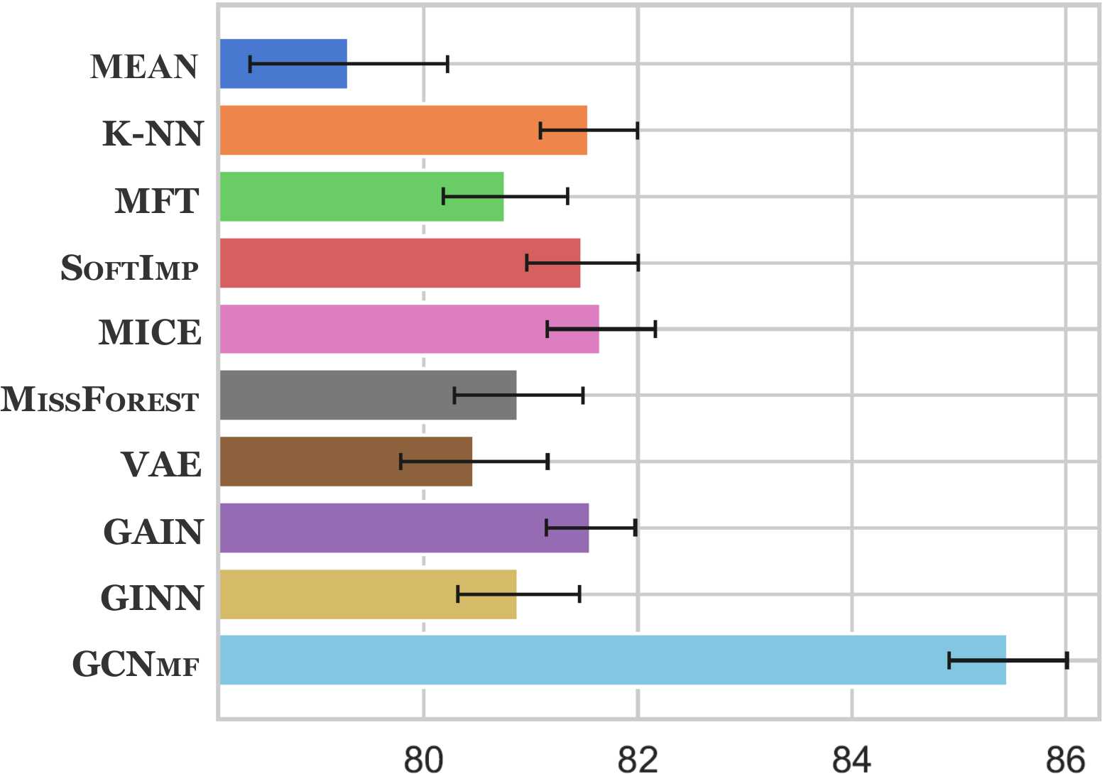
Figure 2 - Figure 3 show the variability of the performance for different methods. We can see that GCNmf is more robust than the baselines, especially in Cora and Citeseer, where there is a high level of variability. Moreover, GCNmf and GCN are on the same level of variability. This implies that representing incomplete features by GMM and calculating the expected activation of neurons do not undermine the robustness of GCN.
| Missing type | Missing rate | 10% | 20% | 30% | 40% | 50% | 60% | 70% | 80% | 90% |
| Uniform Randomly Missing | Mean | 90.72 | 90.41 | 90.10 | 89.79 | 89.11 | 88.40 | 87.13 | 84.47 | 74.97 |
| K-NN | 92.20 | 91.86 | 91.34 | 90.93 | 90.19 | 89.03 | 87.62 | 85.69 | 81.55 | |
| MFT | 92.16 | 91.86 | 91.37 | 90.91 | 90.14 | 88.37 | 86.11 | 84.10 | 79.94 | |
| SoftImp | 90.88 | 90.79 | 90.64 | 90.40 | 89.98 | 89.22 | 88.37 | 86.75 | 84.13 | |
| MICE | – | – | – | – | – | – | – | – | – | |
| MissForest | 92.32 | 92.04 | 91.61 | 90.95 | 90.33 | 89.34 | 88.33 | 86.41 | 82.78 | |
| VAE | 92.23 | 91.91 | 91.33 | 90.54 | 89.28 | 86.98 | 82.52 | 77.74 | 77.27 | |
| GAIN | 92.17 | 91.87 | 91.46 | 91.00 | 90.57 | 89.78 | 89.17 | 88.13 | 86.01 | |
| GINN | 92.15 | 91.96 | 91.62 | 91.00 | 90.28 | 88.94 | 87.66 | 84.73 | 74.90 | |
| GCNmf | 94.09 | 93.50 | 93.05 | 92.40 | 92.29 | 91.79 | 90.77 | 88.32 | 81.46 | |
| Performance gain (%) | 1.92 | 1.59 | 1.56 | 1.54 | 1.90 | 2.24 | 1.79 | 0.22 | -5.29 | |
| | | | | | | | | | | | | | | | | | | ||
| 3.71 | 3.42 | 3.27 | 2.91 | 3.57 | 5.53 | 10.00 | 13.61 | 8.76 | ||
| Biased Randomly Missing | Mean | 92.18 | 92.08 | 92.14 | 91.89 | 91.43 | 91.01 | 89.55 | 87.19 | 76.96 |
| K-NN | 92.17 | 92.06 | 92.02 | 91.83 | 91.47 | 90.92 | 89.84 | 87.85 | 81.65 | |
| MFT | 92.17 | 91.44 | 90.65 | 90.00 | 89.50 | 88.91 | 87.48 | 85.36 | 80.20 | |
| SoftImp | 92.35 | 92.34 | 92.35 | 92.08 | 91.74 | 91.36 | 90.03 | 88.44 | 86.17 | |
| MICE | – | – | – | – | – | – | – | – | – | |
| MissForest | 92.27 | 92.22 | 92.22 | 91.80 | 91.22 | 90.34 | 88.90 | 86.86 | 83.58 | |
| VAE | 92.19 | 92.05 | 91.83 | 91.37 | 90.75 | 89.71 | 87.37 | 84.95 | 76.71 | |
| GAIN | 92.18 | 92.01 | 91.88 | 91.70 | 91.28 | 90.75 | 89.87 | 88.75 | 86.69 | |
| GINN | 92.15 | 92.11 | 92.04 | 91.88 | 91.52 | 90.89 | 89.45 | 87.36 | 75.38 | |
| GCNmf | 94.35 | 94.20 | 93.90 | 93.15 | 92.43 | 91.46 | 90.03 | 86.10 | 81.72 | |
| Performance gain (%) | 2.17 | 2.01 | 1.68 | 1.16 | 0.75 | 0.11 | 0.18 | -2.99 | -5.73 | |
| | | | | | | | | | | | | | | | | | | ||
| 2.39 | 3.02 | 3.59 | 3.50 | 3.27 | 2.87 | 3.04 | 1.35 | 8.41 | ||
| Structurally Missing | Mean | 90.34 | 89.79 | 89.12 | 88.26 | 87.12 | 85.33 | 83.23 | 79.61 | 71.79 |
| K-NN | 91.60 | 91.08 | 90.38 | 89.36 | 88.34 | 87.16 | 85.40 | 82.09 | 76.12 | |
| MFT | 91.51 | 91.00 | 89.95 | 89.11 | 87.36 | 85.81 | 82.90 | 77.73 | 73.72 | |
| SoftImp | 90.29 | 89.67 | 88.86 | 87.86 | 86.77 | 85.36 | 83.07 | 81.53 | 77.38 | |
| MICE | 91.58 | 91.11 | 90.30 | 89.34 | 88.18 | 86.70 | 84.24 | 80.31 | 72.63 | |
| MissForest | 91.57 | 91.05 | 90.23 | 89.36 | 88.34 | 87.16 | 85.40 | 82.09 | 76.22 | |
| VAE | 91.49 | 90.76 | 89.49 | 87.27 | 83.81 | 80.07 | 73.46 | 67.55 | 65.80 | |
| GAIN | 91.60 | 91.08 | 90.38 | 89.36 | 88.34 | 87.16 | 85.40 | 82.09 | 76.12 | |
| GINN | 91.51 | 90.85 | 89.68 | 87.34 | 83.23 | 76.22 | 66.55 | 63.88 | 64.91 | |
| GCNmf | 93.55 | 92.65 | 91.68 | 90.55 | 88.54 | 86.19 | 81.96 | 76.35 | 67.86 | |
| Performance gain (%) | 2.13 | 1.69 | 1.44 | 1.33 | 0.23 | -1.11 | -4.03 | -6.99 | -12.30 | |
| | | | | | | | | | | | | | | | | | | ||
| 3.61 | 3.32 | 3.17 | 3.76 | 6.38 | 13.08 | 23.16 | 19.52 | 4.54 | ||
| GCN | 92.42 | |||||||||
| GCN w/o node features | 85.90 | |||||||||
| Missing type | Missing rate | 10% | 20% | 30% | 40% | 50% | 60% | 70% | 80% | 90% |
| Uniform Randomly Missing | Mean | 89.01 | 88.56 | 88.01 | 87.33 | 86.42 | 85.30 | 83.77 | 81.43 | 75.47 |
| K-NN | 90.00 | 89.60 | 89.10 | 88.34 | 87.32 | 85.68 | 83.39 | 81.16 | 78.60 | |
| MFT | 89.86 | 89.43 | 88.81 | 87.72 | 85.76 | 83.24 | 81.20 | 79.97 | 77.94 | |
| SoftImp | 90.19 | 90.15 | 89.81 | 89.55 | 88.97 | 88.17 | 86.80 | 84.99 | 81.66 | |
| MICE | – | – | – | – | – | – | – | – | – | |
| MissForest | – | – | – | – | – | – | – | – | – | |
| VAE | 89.85 | 89.09 | 88.13 | 87.22 | 85.36 | 83.55 | 80.64 | 74.89 | 64.69 | |
| GAIN | 89.96 | 89.53 | 89.07 | 88.36 | 87.51 | 86.52 | 85.35 | 83.93 | 81.70 | |
| GINN | 90.02 | 89.64 | 89.04 | 87.91 | 86.56 | 84.64 | 83.32 | 81.82 | 77.19 | |
| GCNmf | 93.20 | 92.96 | 92.30 | 92.19 | 90.45 | 90.08 | 88.91 | 87.28 | 83.68 | |
| Performance gain (%) | 3.34 | 3.12 | 2.77 | 2.95 | 1.66 | 2.17 | 2.43 | 2.69 | 2.42 | |
| | | | | | | | | | | | | | | | | | | ||
| 4.71 | 4.97 | 4.87 | 5.70 | 5.96 | 8.22 | 10.26 | 16.54 | 29.36 | ||
| Biased Randomly Missing | Mean | 89.94 | 89.88 | 89.63 | 89.33 | 89.25 | 88.55 | 87.57 | 85.28 | 78.23 |
| K-NN | 90.00 | 89.98 | 89.81 | 89.54 | 89.31 | 88.52 | 87.47 | 84.97 | 78.85 | |
| MFT | 89.98 | 87.50 | 85.88 | 85.07 | 84.32 | 83.76 | 82.85 | 81.54 | 78.23 | |
| SoftImp | 90.31 | 90.25 | 90.23 | 89.99 | 89.90 | 89.03 | 87.12 | 85.96 | 80.63 | |
| MICE | – | – | – | – | – | – | – | – | – | |
| MissForest | – | – | – | – | – | – | – | – | – | |
| VAE | 89.90 | 89.25 | 88.33 | 87.32 | 86.26 | 83.78 | 83.05 | 80.71 | 62.51 | |
| GAIN | 89.97 | 89.87 | 89.60 | 89.32 | 88.89 | 87.85 | 87.00 | 85.05 | 81.95 | |
| GINN | 90.27 | 89.99 | 89.85 | 89.47 | 89.10 | 88.15 | 87.21 | 84.47 | 76.83 | |
| GCNmf | 93.53 | 93.38 | 92.81 | 92.48 | 91.68 | 91.25 | 89.54 | 86.73 | 81.43 | |
| Performance gain (%) | 3.57 | 3.47 | 2.86 | 2.77 | 1.98 | 2.49 | 2.25 | 0.90 | -0.63 | |
| | | | | | | | | | | | | | | | | | | ||
| 4.04 | 6.72 | 8.07 | 8.71 | 8.73 | 8.94 | 8.07 | 7.46 | 30.27 | ||
| Structurally Missing | Mean | 88.16 | 86.95 | 85.76 | 84.20 | 82.43 | 80.83 | 78.92 | 75.79 | 69.76 |
| K-NN | 89.50 | 88.36 | 87.01 | 85.52 | 83.85 | 82.11 | 79.81 | 76.49 | 70.86 | |
| MFT | 89.24 | 87.96 | 86.53 | 84.76 | 83.19 | 80.67 | 78.35 | 75.97 | 72.64 | |
| SoftImp | 89.50 | 88.36 | 87.01 | 85.52 | 83.85 | 82.11 | 79.81 | 76.49 | 70.86 | |
| MICE | – | – | – | – | – | – | – | – | – | |
| MissForest | – | – | – | – | – | – | – | – | – | |
| VAE | 88.57 | 86.83 | 84.32 | 80.96 | 77.49 | 74.01 | 67.84 | 63.06 | 60.39 | |
| GAIN | 89.50 | 88.36 | 87.01 | 85.52 | 83.85 | 82.11 | 79.81 | 76.49 | 70.86 | |
| GINN | 87.48 | 83.35 | 77.50 | 70.06 | 64.31 | 59.45 | 57.95 | 54.88 | 50.81 | |
| GCNmf | 92.23 | 90.54 | 88.77 | 85.74 | 84.78 | 84.59 | 82.00 | 77.21 | 73.31 | |
| Performance gain (%) | 3.05 | 2.47 | 2.02 | 0.26 | 1.11 | 3.02 | 2.74 | 0.94 | 0.92 | |
| | | | | | | | | | | | | | | | | | | ||
| 5.43 | 8.63 | 14.54 | 22.38 | 31.83 | 42.29 | 41.50 | 40.69 | 44.28 | ||
| GCN | 90.25 | |||||||||
| GCN w/o node features | 79.94 | |||||||||
5.2. Link Prediction
The second experiment is for the link prediction task in the Cora and Citeseer citation graphs. We took VGAE (Kipf and Welling 2016) as the base model, which is a variational graph autoencoder and employs GCN as an encoder. We gradually increased the missing rate from 10% to 90% and compare GCNmf against baselines within the base model framework. Following the previous work (Kipf and Welling 2016), we randomly chose 10% edges for testing, 5% edges for validation, and the remaining edges for training; we used a 32-dim hidden layer and 16-dim latent variables in the base model.
Tables 6 and 7 show the average AUC scores obtained by different methods. Bold and underline indicate the best and the second best score for each setting. We also provide the performance results of 1) GCN in the setting of complete features (), and 2) GCN without node features (using the identity matrix instead of the node feature matrix ) as a reference.
We can reach a similar conclusion as the node classification task. GCNmf exhibits the best overall performance. In particular, GCNmf demonstrates excellent performance and is overwhelmingly superior to all baselines in Citeseer; GCNmf outperforms the baselines in most cases in Cora, with only several exceptions when the missing rate reaches high. Again, we can observe the robustness merit of GCNmf, as it even outperforms GCN when the missing rate is low.
We attribute the superiority of GCNmf to the joint learning of GMM and network parameters. Actually, our approach can be understood as calculating the expected activation of neurons over the imputations drawn from missing data density in the first layer. It is the end-to-end joint learning of the parameters that make our approach less likely to converge to sub-optimal solutions.
| Cora | Citeseer | AmaPhoto | AmaComp | |
|---|---|---|---|---|
| MEAN | 1.10 | 1.24 | 12.09 | 14.14 |
| K-NN | 125.04 | 480.19 | 482.73 | 1505.14 |
| MFT | 141.14 | 567.50 | 428.95 | 906.52 |
| SoftImp | 115.15 | 850.55 | 59.26 | 95.14 |
| MICE | – | – | 3879.59 | 6705.73 |
| MissForest | 4039.10 | – | 32528.25 | 48264.58 |
| VAE | 7.91 | 8.64 | 14.23 | 18.78 |
| GAIN | 79.35 | 426.10 | 36.06 | 35.19 |
| GINN | 300.64 | 839.96 | 998.03 | 3199.96 |
| GCNmf | 7.43 (0.59) | 13.52 (2.60) | 22.64 (4.11) | 42.38 (9.75) |
| GCN | 0.86 | 0.91 | 6.82 | 7.79 |
5.3. Running Time Comparison
We compare the running time of different approaches in Table 8. The numbers represent the sum of time for parameter initialization, missing value imputation, and model training. We also provide a reference time of GCN when . We can observe that GCNmf algorithm runs in reasonable time, with model training taking the majority of time (the time for initialization of GMM parameters only accounts for less than ). In comparison, GCNmf is slower than MEAN and VAE, but is much faster than the other seven methods. We note that some imputation techniques suffer due to the high dimension of features. For example, MissForest did not finish within 24 hours in Citeseer.
5.4. Analysis of GCNmf
In this section, we provide study of GCNmf in terms of hyper-parameter sensitivity, optimization analysis, and quality of the reconstructed features.
5.4.1. Hyper-parameter analysis
Figure 4 depicts the performance results with different assignments on the Gaussian components and the number of hidden units in Cora and AmaPhoto datasets. We can observe that the performance reaches a plateau when we have enough number of hidden units to transcribe the information, i.e., for Cora and for AmaPhoto. On the other hand, the performance is not sensitive to , with differences between the best and worst less than when in Cora and when in AmaPhoto, respectively.


5.4.2. Analysis of Optimization
GCNmf employs a joint optimization of GMM and GCN within the same network architecture. Alternatively, we can consider a two-step optimization strategy: in the first step we optimize GMM parameters with input node features using EM algorithm; in the second step we optimize GCN parameters by gradient descent algorithm while fixing the GMM parameters.
We compare the two optimization strategies in Table 9. We can observe that the joint optimization clearly beats the two-step optimization. The advantage becomes greater and greater as the missing rate increases. In particular, when the missing rate becomes high, the two-step optimization fails to learn the “right” model parameters and the performance deteriorates sharply.
| Uniform randomly missnig features | ||||||||||
|---|---|---|---|---|---|---|---|---|---|---|
| Dataset | Missing rate | 10% | 20% | 30% | 40% | 50% | 60% | 70% | 80% | 90% |
| Cora | Joint Opt. | 81.70 | 81.66 | 80.41 | 79.52 | 77.91 | 76.67 | 74.38 | 70.57 | 63.49 |
| Two-step Opt. | 81.50 | 81.43 | 79.81 | 79.35 | 76.75 | 76.04 | 73.97 | 69.16 | 61.46 | |
| Citeseer | Joint Opt. | 70.93 | 70.82 | 69.84 | 68.83 | 67.03 | 64.78 | 60.70 | 55.38 | 47.78 |
| Two-step Opt. | 70.54 | 70.73 | 69.66 | 69.20 | 66.59 | 64.52 | 60.07 | 53.68 | 46.53 | |
| Structurally missing features | ||||||||||
| Dataset | Missing rate | 10% | 20% | 30% | 40% | 50% | 60% | 70% | 80% | 90% |
| AmaPhoto | Joint Opt. | 92.45 | 92.32 | 92.08 | 91.88 | 91.52 | 90.89 | 90.39 | 89.64 | 86.09 |
| Two-step Opt. | 92.49 | 92.23 | 91.90 | 91.40 | 90.73 | 87.94 | 84.93 | 62.46 | 32.44 | |
| AmaComp | Joint Opt. | 86.37 | 86.22 | 85.80 | 85.43 | 85.24 | 84.73 | 84.06 | 80.63 | 73.42 |
| Two-step Opt. | 86.30 | 85.99 | 85.49 | 84.69 | 83.79 | 82.76 | 80.23 | 71.80 | 39.98 | |
5.4.3. Analysis of Reconstructed Node Features
Finally, we conducted a study on how well the reconstructed features by GCNmf. The reconstructed features are the mean of GMM, namely the weighted average of the mean vectors. Figure 5 depicts the Mean Absolute Error (MAE) of the reconstructed features and true features during the training process of the node classification task in AmaPhoto. We can observe that MAE decreases as the number of training epochs increases, and it converges to around 0.35 after 200 epochs. This suggests that the trained GMM captures the density of features more accurately than the initial state optimized by EM algorithm. Although the training aims at learning node labels, it helps to reconstruct the missing features.
6. Conclusion
We proposed GCNmf to supplement a severe deficiency of current GCN models—inability to handle graphs containing missing features. In contrast to the traditional strategy of imputing missing features before applying GCN, GCNmf integrates the processing of missing features and graph learning within the same neural network architecture. Specifically, we propose a novel way to unify the representation of missing features and calculation of the expected activation of the first layer neurons in GCN. We empirically demonstrate that 1) GCNmf is robust against low level of missing features, 2) GCNmf significantly outperforms the imputation based methods in the node classification and link prediction tasks.
Acknowledgements.
This work is partly supported by JSPS Grant-in-Aid for Early-Career Scientists (Grant Number 19K20352), JSPS Grant-in-Aid for Scientific Research(B) (Grant Number 17H01785), JST CREST (Grant Number JPMJCR1687), and the New Energy and Industrial Technology Development Organization (NEDO).References
- (1)
- Abu-El-Haija et al. (2019) Sami Abu-El-Haija, Bryan Perozzi, Amol Kapoor, Hrayr Harutyunyan, Nazanin Alipourfard, Kristina Lerman, Greg Ver Steeg, and Aram Galstyan. 2019. MixHop: Higher-Order Graph Convolution Architectures via Sparsified Neighborhood Mixing. In Proceedings of ICML.
- Akiba et al. (2019) Takuya Akiba, Shotaro Sano, Toshihiko Yanase, Takeru Ohta, and Masanori Koyama. 2019. Optuna: A Next-generation Hyperparameter Optimization Framework. In Proceedings of KDD.
- Bai et al. (2019) Yunsheng Bai, Hao Ding, Song Bian, Ting Chen, Yizhou Sun, and Wei Wang. 2019. Simgnn: A neural network approach to fast graph similarity computation. In Proceedings of WSDM. 384–392.
- Bastings et al. (2017) Joost Bastings, Ivan Titov, Wilker Aziz, Diego Marcheggiani, and Khalil Sima’an. 2017. Graph convolutional encoders for syntax-aware neural machine translation. In Proceedings of EMNLP. 1957–1967.
- Batista et al. (2002) Gustavo EAPA Batista, Maria Carolina Monard, et al. 2002. A Study of K-Nearest Neighbour as an Imputation Method. HIS 87, 251–260 (2002), 48.
- Buuren and Groothuis-Oudshoorn (2010) S van Buuren and Karin Groothuis-Oudshoorn. 2010. mice: Multivariate imputation by chained equations in R. Journal of statistical software (2010), 1–68.
- Che et al. (2018) Zhengping Che, Sanjay Purushotham, Kyunghyun Cho, David Sontag, and Yan Liu. 2018. Recurrent Neural Networks for Multivariate Time Series with Missing Values. Scientific Reports 8, 1 (2018), 6085.
- Chen et al. (2019) Hongxu Chen, Hongzhi Yin, Tong Chen, Quoc Viet Hung Nguyen, Wen-Chih Peng, and Xue Li. 2019. Exploiting centrality information with graph convolutions for network representation learning. In Proceedings of ICDE. 590–601.
- Chen et al. (2018) Jie Chen, Tengfei Ma, and Cao Xiao. 2018. FastGCN: Fast Learning with Graph Convolutional Networks via Importance Sampling. In Proceedings of ICLR.
- Chiang et al. (2019) Wei-Lin Chiang, Xuanqing Liu, Si Si, Yang Li, Samy Bengio, and Cho-Jui Hsieh. 2019. Cluster-GCN: An Efficient Algorithm for Training Deep and Large Graph Convolutional Networks. In Proceedings of KDD. 257–266.
- Choong et al. (2018) Jun Jin Choong, Xin Liu, and Tsuyoshi Murata. 2018. Learning community structure with variational autoencoder. In Proceedings of ICDM. 69–78.
- Cui et al. (2018) Peng Cui, Xiao Wang, Jian Pei, and Wenwu Zhu. 2018. A survey on network embedding. IEEE Transactions on Knowledge and Data Engineering 31, 5 (2018), 833–852.
- Dai et al. (2018) Hanjun Dai, Hui Li, Tian Tian, Xin Huang, Lin Wang, Jun Zhu, and Le Song. 2018. Adversarial Attack on Graph Structured Data (Proceedings of ICML). 1115–1124.
- Dempster et al. (1977) A. P. Dempster, N. M. Laird, and D. B. Rubin. 1977. Maximum Likelihood from Incomplete Data via the EM Algorithm. Journal of the Royal Statistical Society. Series B (Methodological) 39, 1 (1977), 1–38.
- Duvenaud et al. (2015) David K Duvenaud, Dougal Maclaurin, Jorge Iparraguirre, Rafael Bombarell, Timothy Hirzel, Alán Aspuru-Guzik, and Ryan P Adams. 2015. Convolutional networks on graphs for learning molecular fingerprints. In Proceedings of NeurIPS. 2224–2232.
- Fout et al. (2017) Alex Fout, Jonathon Byrd, Basir Shariat, and Asa Ben-Hur. 2017. Protein interface prediction using graph convolutional networks. In Proceedings of NeurIPS. 6530–6539.
- García-Laencina et al. (2010) Pedro J García-Laencina, José-Luis Sancho-Gómez, and Aníbal R Figueiras-Vidal. 2010. Pattern classification with missing data: a review. Neural Computing and Applications 19, 2 (2010), 263–282.
- Glorot and Bengio (2010) Xavier Glorot and Yoshua Bengio. 2010. Understanding the difficulty of training deep feedforward neural networks. In Proceedings of AISTATS. 249–256.
- Hu et al. (2020) Ruiqi Hu, Shirui Pan, Guodong Long, Qinghua Lu, Liming Zhu, and Jing Jiang. 2020. Going Deep: Graph Convolutional Ladder-Shape Networks. In Proceedings of AAAI.
- Ji et al. (2020) Shaoxiong Ji, Shirui Pan, Erik Cambria, Pekka Marttinen, and Philip S. Yu. 2020. A Survey on Knowledge Graphs: Representation, Acquisition and Applications. arXiv:2002.00388
- Jin et al. (2019) Di Jin, Ziyang Liu, Weihao Li, Dongxiao He, and Weixiong Zhang. 2019. Graph convolutional networks meet Markov random fields: Semi-supervised community detection in attribute networks. In Proceedings of AAAI. 152–159.
- Kai Jiang et al. (2005) Kai Jiang, Haixia Chen, and Senmiao Yuan. 2005. Classification for Incomplete Data Using Classifier Ensembles. In Proceedings of ICNNB. 559–563.
- Kingma and Ba (2015) Diederik P. Kingma and Jimmy Ba. 2015. Adam: A Method for Stochastic Optimization. In Proceedings of ICLR.
- Kingma and Welling (2014) Diederik P. Kingma and Max Welling. 2014. Auto-encoding variational bayes. Proceedings of ICLR (2014), 1–14.
- Kipf and Welling (2016) Thomas N Kipf and Max Welling. 2016. Variational Graph Auto-Encoders. NIPS Workshop on Bayesian Deep Learning (2016).
- Kipf and Welling (2017) Thomas N Kipf and Max Welling. 2017. Semi-supervised classification with graph convolutional networks. In Proceedings of ICLR.
- Koren et al. (2009) Y. Koren, R. Bell, and C. Volinsky. 2009. Matrix Factorization Techniques for Recommender Systems. Computer 42, 8 (2009), 30–37.
- Li et al. (2018) Ruoyu Li, Sheng Wang, Feiyun Zhu, and Junzhou Huang. 2018. Adaptive graph convolutional neural networks. In Proceedings of AAAI.
- Li et al. (2019) Steven Cheng-Xian Li, Bo Jiang, and Benjamin Marlin. 2019. Learning from Incomplete Data with Generative Adversarial Networks. In Proceedings of ICLR.
- Liu et al. (2019) Xin Liu, Tsuyoshi Murata, Kyoung-Sook Kim, Chatchawan Kotarasu, and Chenyi Zhuang. 2019. A general view for network embedding as matrix factorization. In Proceedings of WSDM. 375–383.
- Liu et al. (2020) Zhiwei Liu, Yingtong Dou, Philip S. Yu, Yutong Deng, and Hao Peng. 2020. Alleviating the Inconsistency Problem of Applying Graph Neural Network to Fraud Detection. In Proceedings of SIGIR.
- Luo et al. (2018) Yonghong Luo, Xiangrui Cai, Ying ZHANG, Jun Xu, and Yuan xiaojie. 2018. Multivariate Time Series Imputation with Generative Adversarial Networks. In Proceedings of NeurIPS. 1596–1607.
- Maurya et al. (2019) Sunil Kumar Maurya, Xin Liu, and Tsuyoshi Murata. 2019. Fast Approximations of Betweenness Centrality with Graph Neural Networks. In Proceedings of CIKM. 2149–2152.
- Mazumder et al. (2010) Rahul Mazumder, Trevor Hastie, and Robert Tibshirani. 2010. Spectral Regularization Algorithms for Learning Large Incomplete Matrices. J. Mach. Learn. Res. 11 (2010), 2287–2322.
- McAuley et al. (2015) Julian McAuley, Christopher Targett, Qinfeng Shi, and Anton van den Hengel. 2015. Image-Based Recommendations on Styles and Substitutes. In Proceedings of SIGIR. 43–52.
- Narasimhan et al. (2018) Medhini Narasimhan, Svetlana Lazebnik, and Alexander Schwing. 2018. Out of the box: Reasoning with graph convolution nets for factual visual question answering. In Proceedings of NeurIPS. 2654–2665.
- Pan et al. (2018) Shirui Pan, Ruiqi Hu, Guodong Long, Jing Jiang, Lina Yao, and Chengqi Zhang. 2018. Adversarially Regularized Graph Autoencoder for Graph Embedding. In Proceedings of IJCAI. 2609–2615.
- Pelckmans et al. (2005) K. Pelckmans, J. De Brabanter, J.A.K. Suykens, and B. De Moor. 2005. Handling missing values in support vector machine classifiers. Neural Networks 18, 5 (2005), 684–692.
- Perozzi et al. (2014) Bryan Perozzi, Rami Al-Rfou, and Steven Skiena. 2014. DeepWalk: Online Learning of Social Representations. In Proceedings of KDD. 701–710.
- Qiu et al. (2018) Jiezhong Qiu, Yuxiao Dong, Hao Ma, Jian Li, Kuansan Wang, and Jie Tang. 2018. Network embedding as matrix factorization: unifying DeepWalk, LINE, PTE, and node2vec. In Proceedings of WSDM. 459–467.
- Rubin (2004) Donald B Rubin. 2004. Multiple imputation for nonresponse in surveys. Vol. 81. John Wiley & Sons.
- Scarselli et al. (2008) Franco Scarselli, Marco Gori, Ah Chung Tsoi, Markus Hagenbuchner, and Gabriele Monfardini. 2008. The graph neural network model. IEEE Transactions on Neural Networks 20, 1 (2008), 61–80.
- Sen et al. (2008) Prithviraj Sen, Galileo Namata, Mustafa Bilgic, Lise Getoor, Brian Galligher, and Tina Eliassi-Rad. 2008. Collective Classification in Network Data. AI Magazine 29, 3 (2008), 93.
- Shi et al. (2019) Min Shi, Yufei Tang, Xingquan Zhu, and Jianxun Liu. 2019. Feature-Attention Graph Convolutional Networks for Noise Resilient Learning. arXiv:1912.11755
- Shuman et al. (2013) David I Shuman, Sunil K Narang, Pascal Frossard, Antonio Ortega, and Pierre Vandergheynst. 2013. The emerging field of signal processing on graphs: Extending high-dimensional data analysis to networks and other irregular domains. IEEE signal processing magazine 30, 3 (2013), 83–98.
- Simonovsky and Komodakis (2017) Martin Simonovsky and Nikos Komodakis. 2017. Dynamic edge-conditioned filters in convolutional neural networks on graphs. In Proceedings of CVPR. 3693–3702.
- Śmieja et al. (2019) Marek Śmieja, Łukas Struski, Jacek Tabor, and Mateusz Marzec. 2019. Generalized RBF kernel for incomplete data. Knowledge-Based Systems 173 (2019), 150–162.
- Śmieja et al. (2018) Marek Śmieja, Łukasz Struski, Jacek Tabor, Bartosz Zieliński, and Przemysław Spurek. 2018. Processing of missing data by neural networks. In Proceedings of NeurIPS. 2719–2729.
- Smola et al. (2005) Alexander J. Smola, S. V. N. Vishwanathan, and Thomas Hofmann. 2005. Kernel Methods for Missing Variables. In Proceedings of AISTATS.
- Spinelli et al. (2020) Indro Spinelli, Simone Scardapane, and Uncini Aurelio. 2020. Missing Data Imputation with Adversarially-trained Graph Convolutional Networks. Neural Networks 129 (2020), 249–260.
- Stekhoven and Bühlmann (2011) Daniel J. Stekhoven and Peter Bühlmann. 2011. MissForest—non-parametric missing value imputation for mixed-type data. Bioinformatics 28, 1 (2011), 112–118.
- Tang et al. (2015) Jian Tang, Meng Qu, Mingzhe Wang, Ming Zhang, Jun Yan, and Qiaozhu Mei. 2015. Line: Large-scale information network embedding. In Proceedings of WWW. 1067–1077.
- Veličković et al. (2018) Petar Veličković, Guillem Cucurull, Arantxa Casanova, Adriana Romero, Pietro Lio, and Yoshua Bengio. 2018. Graph attention networks. In Proceedings of ICLR.
- Wang et al. (2016) Daixin Wang, Peng Cui, and Wenwu Zhu. 2016. Structural deep network embedding. In Proceedings of KDD. 1225–1234.
- Wang et al. (2017) Q. Wang, Z. Mao, B. Wang, and L. Guo. 2017. Knowledge Graph Embedding: A Survey of Approaches and Applications. IEEE Transactions on Knowledge and Data Engineering 29, 12 (2017), 2724–2743.
- Williams et al. (2005) David Williams, Xuejun Liao, Ya Xue, and Lawrence Carin. 2005. Incomplete-Data Classification Using Logistic Regression. In Proceedings of ICML. 972–979.
- Wu et al. (2020) Z. Wu, S. Pan, F. Chen, G. Long, C. Zhang, and P. S. Yu. 2020. A Comprehensive Survey on Graph Neural Networks. IEEE Transactions on Neural Networks and Learning Systems (2020), 1–21.
- Yang et al. (2019) Liang Yang, Zesheng Kang, Xiaochun Cao, Di Jin, Bo Yang, and Yuanfang Guo. 2019. Topology Optimization based Graph Convolutional Network. In Proceedings of IJCAI. 4054–4061.
- Yang et al. (2020) Liang Yang, Fan Wu, Junhua Gu, Chuan Wang, Xiaochun Cao, Di Jin, and Yuanfang Guo. 2020. Graph Attention Topic Modeling Network. In Proceedings of The Web Conference. 144–154.
- Yang et al. (2016) Zhilin Yang, William W. Cohen, and Ruslan Salakhutdinov. 2016. Revisiting Semi-Supervised Learning with Graph Embeddings. In Proceedings of ICML. 40–48.
- Yi et al. (2020) Joonyoung Yi, Juhyuk Lee, Sungju Hwang, and Eunho Yang. 2020. Why Not to Use Zero Imputation? Correcting Sparsity Bias in Training Neural Networks. In Proceedings of ICLR.
- Ying et al. (2018) Rex Ying, Ruining He, Kaifeng Chen, Pong Eksombatchai, William L Hamilton, and Jure Leskovec. 2018. Graph convolutional neural networks for web-scale recommender systems. In Proceedings of KDD. 974–983.
- Yoon et al. (2018) Jinsung Yoon, James Jordon, and Mihaela van der Schaar. 2018. GAIN: Missing Data Imputation using Generative Adversarial Nets. In Proceedings of ICML, Vol. 80. 5689–5698.
- Zhang et al. (2018) Muhan Zhang, Zhicheng Cui, Marion Neumann, and Yixin Chen. 2018. An end-to-end deep learning architecture for graph classification. In Proceedings of AAAI.
- Zhou et al. (2018) Jie Zhou, Ganqu Cui, Zhengyan Zhang, Cheng Yang, Zhiyuan Liu, Lifeng Wang, Changcheng Li, and Maosong Sun. 2018. Graph neural networks: A review of methods and applications. arXiv:1812.08434 (2018).
- Zhu et al. (2019) Dingyuan Zhu, Ziwei Zhang, Peng Cui, and Wenwu Zhu. 2019. Robust Graph Convolutional Networks Against Adversarial Attacks. In Proceedings of KDD. 1399–1407.
- Zügner et al. (2018) Daniel Zügner, Amir Akbarnejad, and Stephan Günnemann. 2018. Adversarial Attacks on Neural Networks for Graph Data. In SIGKDD. 2847–2856.
- Zügner and Günnemann (2019) Daniel Zügner and Stephan Günnemann. 2019. Certifiable robustness and robust training for graph convolutional networks. In Proceedings of KDD. 246–256.