Plasmonic Tuning of the Near Field Heat Transfer in Double Layer GraphenePreprint: APS/123-QED????????????

Heat transfer between two bodies may greatly exceed the black-body radiation limit in the near field regime. The effect is due to the non-radiative, evanescent modes of the electromagnetic field Pendry 1999, which can transfer energy between closely spaced dielectric Polder and Van Hove 1971; Loomis and Maris 1994; Pendry 1999; Volokitin and Persson 2007, or metallic Mahan 2017; Levin et al. 1980; Kamenev 2018; Wise et al. 2020 surfaces. Specifically in metals, the near field heat transfer (NFHT) is associated with the Coulomb interactions between thermally excited electron-hole pairs Zhang et al. 2018; Jiang and Wang 2017; Mahan 2017. The resonant modes of the Coulomb coupled electron-hole plasmas – the surface plasmons – may be expected to play an important role in this process, offering a higher efficiency and tunability of the heat transfer Mulet et al. 2001; Volokitin and Persson 2003; Volokitin and Persson 2004. Yet in conventional metals, plasmons play a modest role, dominating the heat transport only in a narrow range of temperatures and scattering rates Wise et al. 2020.

Graphene is a promising material Novoselov et al. 2004; Novoselov et al. 2005, which allows for a high degree of control over its plasmon spectra, through electrostatic doping, temperature and choice of the spacer Grigorenko et al. 2012; Koppens et al. 2011; Low and Avouris 2014. Due to the Dirac point in its electronic spectrum, graphene supports unusual plasmon modes Hwang and Das Sarma 2007; Hwang and Das Sarma 2009; Vafek 2006; Schütt et al. 2011, which could serve as mediators of the inter-layer heat transfer. The role of plasmons in NFHT between two graphene layers was highlighted in Refs. [Svetovoy et al. 2012] and [Ilic et al. 2012], who presented numerical evidence for the effect. It was shown that NFHT between the two graphene layers can be greatly enhanced by a factor of $10^{2}\sim 10^{3}$ compared to the black body radiation at room temperature.

In this article, we take a kinetic approach Kamenev 2011; Jiang and Wang 2017; Zhang et al. 2018; Wise et al. 2020. The energy transfer is captured by the energy exchange during the electron-electron scattering and the processes of the creation and annihilation of the electron-hole pairs in the two layers. This approach allows us to analyze the problem analytically and extract the parametric dependence (such as temperature, $T$, and interlayer distance, $d$) for various heat transfer channels. Here we focus on the plasmon channel, which dominates NFHT in graphene through a broad range of the relevant parameters.

We consider two graphene layers kept at different temperatures as shown in Fig. 1. The electrons in the two layers interact through the screened Coulomb potential. As a result, the electron density fluctuations of the two graphene layers are strongly coupled. This leads to the two plasmon branches - the optical and acoustic plasmons, corresponding to the in-phase and the out-of-phase oscillations of the electron densities respectively. Their dispersion relations are shown in Fig. 3. The plasmon mediated NFHT conductance as a function of temperature is summarized in Fig. 4. At small temperature it exhibits $T^{3}$ dependence, which is similar to the radiative Stefan–Boltzmann law. The coefficient however is greatly exceeding the Stefan–Boltzmann one, as the the speed of light (in the negative two power) is substituted with the graphene Fermi velocity, $v_{F}$. The thermal conductance riches a broad maximum at $T\approx v_{F}/d$ and slowly decrease as $T^{-1/2}$ at higher temperatures.

Such non-monotonic thermal conductance is a signature of an undoped graphene. In a doped case the maximum is sharply suppressed once the chemical potential, $\mu$, exceeds the characteristic temperature $v_{F}/d$. This opens a way to manipulate the heat transport by purely electrostatic means. Indeed, applying a small voltage between the two graphene layers, or between a graphene layer and a gate, one can induce a charge density and thus non-zero chemical potential. We show that a minute voltage is sufficient to decrease the heat transfer exponentially.

In the second order in the dynamically screened interlayer Coulomb interactions (RPA approximation), the net heat flux between the two layers with temperatures $T_{1}$ and $T_{2}$ is given by Pendry 1999; Mahan 2017; Bimonte et al. 2017; Jiang and Wang 2017; Zhang et al. 2018; Kamenev 2018; Caroli et al. 1971:

where the integration runs over the 2D momentum, $\boldsymbol{q}$, and energy, $\omega$. Here $N_{j}(\omega)=\omega/\left[\exp(\omega/T_{j})-1\right]$ and $\Pi_{j}(q,\omega)$ are the Planck function and the polarization operator, Fig. 2(a), with $j=1,2$ labeling the layers. Finally, $U_{12}(q,\omega)$ is the screened interlayer Coulomb interaction, which may be written as:

where $v_{F}$ and $\alpha_{g}=e^{2}/(\hbar v_{F}\tilde{\epsilon})$ are the Fermi velocity of the Dirac spectrum and the fine structure constant in graphene, respectively; $\tilde{\epsilon}$ is the dielectric constant of a spacer between the two layers and $d$ is the interlayer separation. Within the RPA approximation the interlayer dielectric function, $\epsilon_{12}(q,\omega)$, is given by the solution of the $2\times 2$ matrix Dyson’s equation Altland and Simons 2010; Das Sarma and Madhukar 1981:

As explained below, the main contribution to NFHT in graphene is coming from the resonances (poles) of the dynamically screened interactions, $U_{12}(q,\omega)$ Mulet et al. 2001; Volokitin and Persson 2003; Volokitin and Persson 2004; Wise et al. 2020. These plasmon resonances at, in general, complex frequency, $\omega=\omega_{\text{P}}(q)-i\Gamma_{\text{P}}(q)$, are determined by zeros of the dielectric function, $\epsilon_{12}(q,\omega)=0$. In a vicinity of the plasmon pole the screened interaction takes the form

where $\omega_{\text{P}}(q)$ and $\Gamma_{\text{P}}(q)$ are the plasmon frequency and the decay rate, and $Z(q)$ is the residue of the plasmon propagator. For the underdamped plasmons, with $\Gamma_{\text{P}}(q)\ll\omega_{\text{P}}(q)$, one can evaluate the frequency integral in Eq. (1) in the pole approximation Flensberg and Hu 1995; Narozhny and Levchenko 2016 to single out the plasmon contribution to the heat flux:

It is clear from here that the plasmon part of the heat flux is weighted by $\Im\Pi_{j}(q,\omega_{\text{P}}(q))$. This is the reason why plasmons do not play a role in conventional metals at low temperatures Kamenev 2018; Wise et al. 2020; Mahan 2017; Stern 1967. Indeed, the 2D plasmon frequency, $\omega_{\text{P}}(q)\propto\sqrt{q}$ Giuliani and Vignale 2005 satisfies $\omega_{\text{P}}(q)\gg v_{F}q$. On the other hand, at $T=0$ all particle-hole excitations have $\omega\leq v_{F}q$, resulting in $\Im\Pi_{j}(q,\omega_{\text{P}}(q))=0$. At a finite temperature $\Im\Pi_{j}(q,\omega_{\text{P}}(q))\propto\exp\{-\epsilon_{F}/T\}$ Stern 1967 and thus the plasmon contribution is still small. It may become significant, however at $T>v_{F}/l$ and $d\sim l$, in disordered metals with $l$ being the mean free path Wise et al. 2020.

Undoped graphene is qualitatively different. Due to the inter-band transitions, Fig. 2(b), there are particle-hole excitations with $\omega\geq v_{F}q$, i.e. $\Im\Pi_{j}(q,\omega_{\text{P}}(q))\neq 0$, even at $T=0$. This is the reason why the plasmon contribution, Eq. (5), dominates the heat transfer in the undoped graphene bilayers. To make the quantitative predictions let us review the plasmon dispersion and damping in graphene bilayers.

We are interested in the frequency range $v_{F}q<\omega\lesssim T_{j}$. The first inequality specifies the range where underdamped plasmons may exist. The second one follows from the fact that the Planck functions in Eq. (5) limit the frequency integration by the temperature. In this range, the graphene polarization operator, Fig. 2(a), is given by Schütt et al. 2011:

where $N$ is the Dirac cone degeneracy ($N=4$ for graphene due to two spins and two valleys). As mentioned above, the high frequency, $\omega>v_{F}q$, polarization operator has a finite imaginary part. This is a direct result of having the inter-band electron-hole excitations near the Dirac point, shown in Fig. 2(b). Hence, graphene is a good emitter/absorber of high frequency modes, such as plasmons.

The double layer system supports two modes called Hwang and Das Sarma 2009 optical (OP) and acoustic plasmon (AP). Their complex frequencies follow from $\epsilon_{12}(q,\omega)=0$, with the dielectric function given by Eq. (3) and the polarization operators given by Eq. (6). As detailed in the Supplemental Material Sup, their dispersions are, Fig. 3:

These expressions hold for $q<d^{-1}$, while in the opposite limit Eqs. (7) smoothly connect to the plasmon frequencies of each individual graphene layer Vafek 2006; Schütt et al. 2011.

The OP corresponds to in-phase oscillations of the electron densities. Its dispersion relation, Eq. (7a), is similar to the plasmon frequency of a single graphene layer Vafek 2006; Schütt et al. 2011. For $v_{F}q<N\alpha_{g}(T_{1}+T_{2})$, the OP exhibits a square root dispersion, $\omega_{\text{OP}}(q)\approx\sqrt{\ln 2N\alpha_{g}(T_{1}+T_{2})v_{F}q}$; while at larger momenta, $v_{F}q>N\alpha_{g}(T_{1}+T_{2})$, it has a linear spectrum $\omega_{\text{OP}}(q)\approx v_{F}q$, Fig. 3. The AP mode corresponds to out-of-phase, charge neutral oscillations, thus the linear dispersion, Eq. (7b), Fig. 3. Notice that the AP is only under-damped at a high enough temperature, so that its velocity is larger than $v_{F}$ Hwang and Das Sarma 2009, $T_{1,2}>v_{F}(N\alpha_{g}d)^{-1}$. In the opposite limit the AP mode merges with the intra-band single particle excitations and is over-damped.

The plasmon decay rate, $\Gamma_{\text{P}}(q)$, and the residue of the plasmon propagator, $Z(q)$, can be written as:

where $s_{\text{P}}=s_{\text{OP}/AP}=\pm 1$ is a sign related to the plasmon species. The ratio between the plasmon decay rate and its frequency is much less than one, Fig. (3), through the entire range, $\omega_{\text{P}}(q)\lesssim T$, contributing to the heat current. Therefore, the plasmon modes are indeed underdamped, justifying Eq. (5).

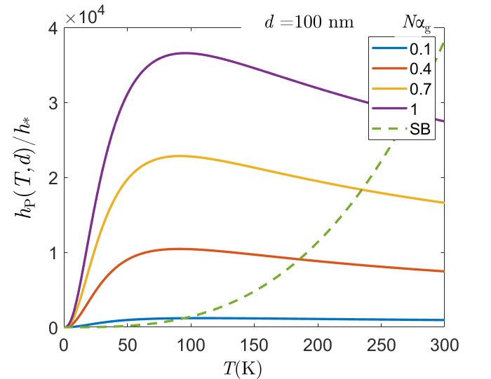
Employing Eq. (5) along with Eqs. (7)-(8), one finds the plasmon contribution to NFHT. We present results, Fig. 4, for the heat transfer conductance Ilic et al. 2018:

which can be measured through the temperature relaxation time: $\tau(T,d)=C(T)/2h_{\text{P}}(T,d)$, where $C(T)$ is the specific heat of the undoped graphene Pop et al. 2012. In the limit $N\alpha_{g}\ll 1$, one can identify the three temperature regimes, where the asymptotic analytic expressions are available in Supplemental Material Sup, cf. Fig. 4,

At low temperatures, $T<v_{F}/(N\alpha_{g}d)$, only OP mode is underdamped, while in the opposite limit both OP and AP modes are underdamped and yield comparable contributions to NFHT conductance. For $T<v_{F}/d$ the integral in Eq. (5) is cut by the Planck function, limiting the relevant momenta by $v_{F}q<T$. As a result, the heat transfer conductance follows $h\sim(N\alpha_{g})^{2}T^{3}/v^{2}_{F}$ – the Stefan-Boltzmann like relation (the latter describes the far-field radiation and is given by $h_{\mathrm{SB}}\sim T^{3}/c^{2}$). There is no dependence on the separation, $d$, between the layers in this regime. In the intermediate temperature range, the inverse layer separation, $d^{-1}$, effectively limits the momentum integral, $v_{F}q<v_{F}d^{-1}<T$ making the heat conductance temperature independent, but $\propto(v_{F}/d)^{3}$ instead. Notice that to observe the high temperature regime of Eq. (10), it’s necessary to have $N\alpha_{g}>(v_{F}/c)^{2/5}\approx 0.1$, otherwise the Stefan-Boltzmann far-field radiation mechanism is more important than NFHT, Fig. 4.

We have found that NFHT conductance in the undoped graphene double layers follows a characteristic non-monotonic temperature dependence, Fig. 4. It reaches a broad maximum at $T_{m}\approx v_{F}/d$ and slowly decreases at higher temperature, before the radiative transfer kicks in at $\approx 4T_{m}(N\alpha_{g})^{3/7}$. Throughout the low temperature range, $T\leq T_{m}$, the NFHT in graphene greatly exceeds that in conventional metals Kamenev 2018; Wise et al. 2020; Mahan 2017. The corresponding enhancement factor is $(N\alpha_{g}\kappa d)^{2}\gg 1$, where $\kappa\gtrsim 1nm^{-1}$ is the inverse screening radius in metals. In fact, at the maximum, $T\approx T_{m}$, the graphene NFHT is only a factor of $(N\alpha_{g})^{2}$ off the Pendry’s boundary Pendry 1999 for the maximal possible heat flux.

The plasmon contribution to the heat flux can be switched off by electrostatic gating. Notice that a voltage, $V$, applied between the two graphene layers induces the charge densities $n=\pm\tilde{\epsilon}\,V/(ed)$ in the two layers, measured from the charge neutrality point. The chemical potential of each graphene layer changes to $\pm\mu$, accordingly. There is a characteristic gate voltage, $V_{\text{T}}=0.23\times\frac{N\alpha_{g}}{e}\frac{dT^{2}}{v_{F}}$, when the chemical potential is equal to the temperature, $\mu=T$. For a smaller gate voltage, $V\lesssim V_{\text{T}}$, the chemical potential is smaller than temperature, $\mu\approx T\times V/V_{\text{T}}<T$. In this case, the plasmon contribution to the NFHT, Eq. (10) is basically intact. At a larger gate voltage, $V\gtrsim V_{\text{T}}$, the chemical potential is greater than the temperature, $\mu\approx 1.7\times T\sqrt{V/V_{\text{T}}}>T$. In this case, the imaginary part of the polarization operator, $\Im\Pi(q,\omega_{P}(q))\sim\exp\left[-\mu/T\right]$, is exponentially small Hwang and Das Sarma 2007. As discussed before, the heat transfer conductance is proportional to the imaginary part of the polarization operator, $h\sim\left(\Im\Pi\right)^{2}/\Gamma_{\text{P}}$, (where $\Gamma_{\text{P}}\sim\Im\Pi$). Hence, the plasmon contribution to the NFHT is exponentially small, $h\sim\exp\left[-1.7\sqrt{V/V_{\text{T}}}\right]$ for $V>V_{\text{T}}$. Therefore the plasmon contribution to NFHT is effectively switched off by the gate voltage $V_{\text{T}}$. For a typical inter-layer separation $d=100\text{ nm}$, it is given by $V_{\text{T}}=0.026\times\left(\frac{T}{10\text{K}}\right)^{2}\text{ meV}$. Thus the small electrostatic potential may be used to tune on and off the heat flux in the graphene double layers.

We are grateful to D. Basko, I. Gorny, A. Levchenko, O. Ilic, M. Sammon, J. Schmalian, and H. Yeh for useful discussions. This research was supported by NSF Grant No. DMR-1608238 and partly by the Heising-Simons Foundation, the Simons Foundation, and NSF Grant No. NSF PHY-1748958.

References

- Pendry (1999) J. Pendry, J. Phys.: Condens. Matter 11, 6621 (1999).
- Polder and Van Hove (1971) D. Polder and M. Van Hove, Phys. Rev. B 4, 3303 (1971).
- Loomis and Maris (1994) J. J. Loomis and H. J. Maris, Phys. Rev. B 50, 18517 (1994).
- Volokitin and Persson (2007) A. I. Volokitin and B. N. J. Persson, Rev. Mod. Phys. 79, 1291 (2007).
- Mahan (2017) G. D. Mahan, Phys. Rev. B 95, 115427 (2017).
- Levin et al. (1980) M. Levin, V. Polevoy, and S. Rytov, Zh. eksp. i teoret. fiz 79 (1980).
- Kamenev (2018) A. Kamenev, arXiv:1811.10187 (2018).
- Wise et al. (2020) J. L. Wise, D. M. Basko, and F. W. Hekking, arXiv:2002.00627 (2020).
- Zhang et al. (2018) Z.-Q. Zhang, J.-T. Lü, and J.-S. Wang, Phys. Rev. B 97, 195450 (2018).
- Jiang and Wang (2017) J.-H. Jiang and J.-S. Wang, Phys. Rev. B 96, 155437 (2017).
- Mulet et al. (2001) J.-P. Mulet, K. Joulain, R. Carminati, and J.-J. Greffet, Appl. Phys. Lett. 78, 2931 (2001).
- Volokitin and Persson (2003) A. I. Volokitin and B. Persson, JETP Lett. 78, 457 (2003).
- Volokitin and Persson (2004) A. I. Volokitin and B. N. J. Persson, Phys. Rev. B 69, 045417 (2004).
- Novoselov et al. (2004) K. S. Novoselov, A. K. Geim, S. V. Morozov, D. Jiang, Y. Zhang, S. V. Dubonos, I. V. Grigorieva, and A. A. Firsov, Science 306, 666 (2004).
- Novoselov et al. (2005) K. S. Novoselov, A. K. Geim, S. Morozov, D. Jiang, M. Katsnelson, I. Grigorieva, S. Dubonos, Firsov, and AA, Nature (London) 438, 197 (2005).
- Grigorenko et al. (2012) A. N. Grigorenko, M. Polini, and K. S. Novoselov, Nat. Photon. 6, 749 (2012).
- Koppens et al. (2011) F. H. Koppens, D. E. Chang, and F. J. Garcia de Abajo, Nano Lett. 11, 3370 (2011).
- Low and Avouris (2014) T. Low and P. Avouris, ACS Nano 8, 1086 (2014).
- Hwang and Das Sarma (2007) E. H. Hwang and S. Das Sarma, Phys. Rev. B 75, 205418 (2007).
- Hwang and Das Sarma (2009) E. H. Hwang and S. Das Sarma, Phys. Rev. B 80, 205405 (2009).
- Vafek (2006) O. Vafek, Phys. Rev. Lett. 97, 266406 (2006).
- Schütt et al. (2011) M. Schütt, P. M. Ostrovsky, I. V. Gornyi, and A. D. Mirlin, Phys. Rev. B 83, 155441 (2011).
- Svetovoy et al. (2012) V. B. Svetovoy, P. J. van Zwol, and J. Chevrier, Phys. Rev. B 85, 155418 (2012).
- Ilic et al. (2012) O. Ilic, M. Jablan, J. D. Joannopoulos, I. Celanovic, H. Buljan, and M. Soljačić, Phys. Rev. B 85, 155422 (2012).
- Kamenev (2011) A. Kamenev, Field theory of Non-equilibrium Systems (Cambridge University Press, Cambridge, 2011).
- Bimonte et al. (2017) G. Bimonte, T. Emig, M. Kardar, and M. Krüger, Ann. Rev. Condens. Matter Phys. 8, 119 (2017).
- Caroli et al. (1971) C. Caroli, R. Combescot, P. Nozieres, and D. Saint-James, J. Phys. C 4, 916 (1971).
- Altland and Simons (2010) A. Altland and B. D. Simons, Condensed matter field theory (Cambridge university press, 2010).
- Das Sarma and Madhukar (1981) S. Das Sarma and A. Madhukar, Phys. Rev. B 23, 805 (1981).
- Flensberg and Hu (1995) K. Flensberg and B. Y.-K. Hu, Phys. Rev. B 52, 14796 (1995).
- Narozhny and Levchenko (2016) B. N. Narozhny and A. Levchenko, Rev. Mod. Phys. 88, 025003 (2016).
- Stern (1967) F. Stern, Phys. Rev. Lett. 18, 546 (1967).
- Giuliani and Vignale (2005) G. Giuliani and G. Vignale, Quantum theory of the electron liquid (Cambridge university press, 2005).
- (34) Supplemental Material .
- Ilic et al. (2018) O. Ilic, N. H. Thomas, T. Christensen, M. C. Sherrott, M. Soljaěić, A. J. Minnich, O. D. Miller, and H. A. Atwater, ACS Nano 12, 2474 (2018).
- Pop et al. (2012) E. Pop, V. Varshney, and A. K. Roy, MRS Bulletin 37, 1273 (2012).