Dynamics of SIR model with vaccination and heterogeneous behavioral response of individuals modeled by the Preisach operator Thanks: The work of Jana Kopfová and Petra Petra Nábělková was supported by the institutional support for the development of research organizations IČ 47813059.

In Chladná et al. 2020, the relationship between the density of the infected population, $I=I(t)$, and the vaccination rate was modeled by the simplest hysteretic operator called the non-ideal relay, which is also known as a rectangular hysteresis loop or a lazy switch (Visintin 1994). The relay operator is characterized by two scalar parameters $\alpha_{1}$ and $\alpha_{2}$, the threshold values, with $\alpha_{1}<\alpha_{2}$. We will use the notation $\alpha=(\alpha_{1},\alpha_{2})$. The input of the relay is an arbitrary continuous function of time, $I:\mathbb{R}_{+}\to\mathbb{R}$. The state $\nu_{\alpha}(\cdot)$ equals either $0$ or $1$ at any moment $t\in\mathbb{R}_{+}$. If the input value at some instant is below the lower threshold value $\alpha_{1}$, then the state at this instant is $0$ and it remains equal to $0$ as long as the input is below the upper threshold value $\alpha_{2}$. When the input reaches the value $\alpha_{2}$, the state switches instantaneously to the value $1$. Then, the state remains equal to $1$ as long as the input stays above the lower threshold value $\alpha_{1}$. When the input reaches the value $\alpha_{1}$, the state switches back to $0$. This dynamics is captured by the input-state diagram shown in Figure 1. In particular, the input-state pair $(I(t),\nu_{\alpha}(t))$ belongs to the union of the two horizontal rays shown in bold in Figure 1 at all times.

The above description results in the following definition. Given any continuous input $I:\mathbb{R}_{+}\to\mathbb{R}$ and an initial value of the state, $\nu_{\alpha}(0)=\nu_{\alpha}^{0}$, satisfying the constraints

the state of the relay at the future moments $t>0$ is defined by

This time series of the state, which depends both on the input $I(t)$ $(t\geq 0)$ and the initial state $\nu_{\alpha}(0)=\nu_{\alpha}^{0}$ of the relay, will be denoted by

By definition, the state satisfies the constraints

at all times. Further, the function (7) has at most a finite number of jumps between the values $0$ and $1$ on any finite time interval $t_{0}\leq t\leq t_{1}$. If the input oscillates between two values $I_{1},I_{2}$, such that $I_{1}<\alpha_{1}<\alpha_{2}<I_{2}$, then the point $(I(t),\nu_{\alpha}(t))$ moves counterclockwise along the rectangular hysteresis loop shown in Figure 1.

In Chladná et al. (2020), it was assumed that interventions of the health authority change the vaccination rate according to the following rules. The vaccination rate is switched from a lower rate $v_{nat}$ to a higher rate ${v_{int}:=v_{nat}+q_{0}}$, ${q_{0}>0}$, when the density of the infected population reaches a threshold value $\alpha_{2}$. The intervention stops when the number of infected individuals drops below a lower threshold value $\alpha_{1}$, at which point the vaccination rate returns to its lower value $v_{nat}$. Using the definition (7) of the non-ideal relay operator (8), this leads to the formula

Coupling of this operator equation with dynamic equations (3) results in a switched system.

As shown in Chladná et al. (2020), switched system (3), (10) exhibits different dynamic scenarios depending on its parameters. In particular, it can have a globally stable endemic equilibrium. Alternatively, a locally stable endemic equilibrium coexists with a stable periodic orbit. Along this orbit, the vaccination rate (10) switches between the values $v_{nat}$ and $v_{nat}+q_{0}$ twice per period.

Now, we consider a model, in which several vaccination laws of the form (10), with different thresholds $\alpha$, are combined either because the health authority employs multiple intervention strategies or because different individuals respond differently to the advent of an epidemic.

Assume that the health authority has multiple intervention policies (numbered $n=1,\ldots,N$) in place, each increasing the vaccination rate by a certain amount $q_{n}$ while the intervention is implemented, in order to provide a response, which is adequate to the severity of the epidemic. Further, assume that each intervention policy is guided by the two-threshold start/stop rule, such as in (10), associated with a particular pair of thresholds $\alpha^{n}=(\alpha_{1}^{n},\alpha_{2}^{n})$. Under these assumptions, the vaccination rate in system (3) is given by

This formula defines a mapping from the space of continuous inputs $I:\mathbb{R}_{+}\to\mathbb{R}$ to the space of piecewise constant outputs $v:\mathbb{R}_{+}\to\mathbb{R}$, which is known as the discrete Preisach operator ( Krasnosel’skii et al. 1983), see Figure 2. In particular, the vaccination rate (11) is set to change at multiple thresholds $\alpha_{1}^{n},\alpha_{2}^{n}$.

On the other hand, individuals can respond differently to dynamics of the epidemic and interventions of the health authority. In particular, the willingness to receive vaccination can vary significantly from individual to individual for the same level of threat of contracting the disease. In order to account for the heterogeneity of the individual response, let us divide the susceptible population into non-intersecting subpopulations parametrized by points $\alpha$ of a subset $\Pi\subset\{\alpha=(\alpha_{1},\alpha_{2}):\alpha_{1}<\alpha_{2}\}$ of the $\alpha$-plane. Assuming that the vaccination rate for a subpopulation labeled $\alpha$ is given by (10) with $q=q(\alpha)$, the total vaccination rate equals

where the probability measure $F$ describes the distribution of the susceptible population over the index set $\Pi$ (the set of threshold pairs). As a simplification, let us assume that this measure is independent of time (in particular, the distribution does not change with variations of $I$). Then, the mapping of the space of continuous inputs $I:\mathbb{R}_{+}\to\mathbb{R}$ to the space of outputs $v:\mathbb{R}_{+}\to\mathbb{R}$ defined by (12) is known as the general Preisach operator, which includes the discrete Preisach operator (11) and a continuous Preisach model (corresponding to an absolutely continuous measure $F$) as particular cases. In either case, the Preisach operator is referred to as a superposition (or parallel connection) of weighted non-ideal relays.

Let us consider a rigorous definition of the Preisach operator (12) with an absolutely continuous measure $F$ (Krasnosel’skii et al., 1989). It involves a collection of non-ideal relays ${\mathcal{R}}_{\alpha}$, which respond to the same continuous input $I=I(t)$ independently. The relays contributing to the system have different pairs of thresholds $\alpha=(\alpha_{1},\alpha_{2})\in\Pi$, where we assume that $\Pi$ is measurable and bounded; the $\alpha$-plane is called the Preisach plane. The output of the continuous Preisach model is the scalar-valued function

where $q:\Pi\to\mathbb{R}$ is a positive bounded measurable function (measure density) representing the weights of the relays; and, $\nu_{\alpha}^{0}$ is the initial state of the relay ${\mathcal{R}}_{\alpha}$ for any given $\alpha\in\Pi$. The function $\nu^{0}=\nu_{\alpha}^{0}:\Pi\to\{0,1\}$ of the variable $\alpha=(\alpha_{1},\alpha_{2})$ is referred to as the initial state of the Preisach operator. It is assumed to be measurable and satisfy the constraints (5), (6), in which case the initial state-input pair is called compatible. These requirements ensure that the integral in (13) is well-defined for each $t\geq 0$ and, furthermore, the output $v(\cdot)$ of the Preisach model is continuous. The input-output operator of the Preisach model defined by (13) will be denoted by

where both the input $I:\mathbb{R}_{+}\to\mathbb{R}$ and the initial state $\nu^{0}=\nu^{0}_{\alpha}$ (which is compatible with the input) are the arguments; the value of this operator is the output $v:\mathbb{R}_{+}\to\mathbb{R}$.

In what follows we consider system (3) with the vaccination rate defined by equation (13).

The Preisach operator (14) is globally Lipschitz continuous (Krasnosel’skii et al. 1983). More precisely, the relations

imply

for any $\tau\geq 0$ with

Let us denote by $\mathfrak{U}$ the set of all triplets $(I_{0},S_{0},\nu^{0})$, where $(I_{0},S_{0})\in\mathfrak{D}$ (see (4)) and the initial state $\nu^{0}$ of the Preisach operator is compatible with $I_{0}$. The global Lipschitz estimate (15) ensures (for example, using the Picard-Lindelöf type of argument) that for given $(I_{0},S_{0},\nu^{0})\in\mathfrak{U}$, system (3) with the Preisach operator (14) has a unique local solution with the initial data $I(0)=I_{0},S(0)=S_{0}$ and the initial state $\nu^{0}$ (see, for example, the survey in Leonov et al. 2017). Further, the invariance of $\mathfrak{D}$ implies that each solution is extendable to the whole semi-axis $t\geq 0$. These solutions induce a semi-flow in the set $\mathfrak{U}$, which is considered to be the phase space of system (3) and is endowed with a metric by the natural embedding into the space $\mathbb{R}^{2}\times L_{1}(\Pi;\mathbb{R})$. This leads to the standard definition of local and global stability including stability of equilibrium states and periodic solutions. In particular, an equilibrium is a triplet $(I_{0},S_{0},\nu^{0})\in\mathfrak{U}$ and a periodic solution is a periodic function $(I(\cdot),S(\cdot),\nu(\cdot)):\mathbb{R}_{+}\to\mathfrak{U}$ where the last component viewed as a function $\nu:\mathbb{R}_{+}\times\Pi\to\{0,1\}$ of two variables $t\in\mathbb{R}_{+}$ and $\alpha\in\Pi$ is given by (8).

The vaccination rate (13) at an equilibrium is constant, while for a periodic solution the vaccination rate is also periodic with the period of $I$ and $S$.

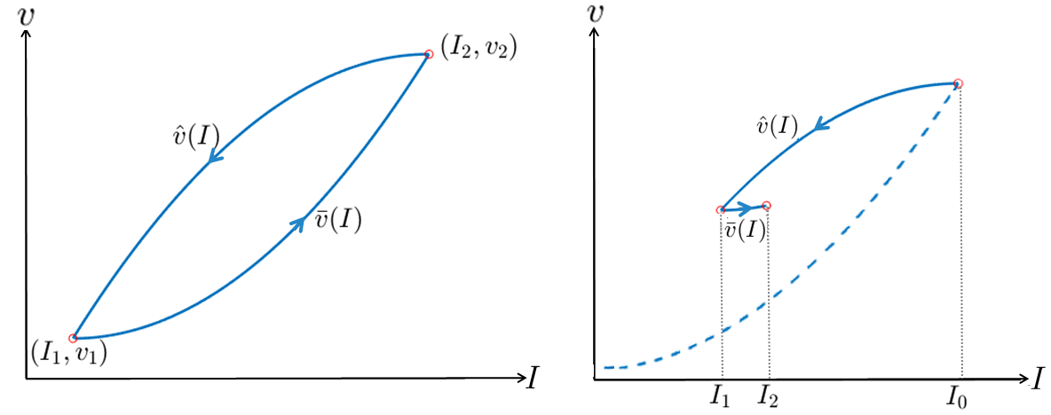
We call a periodic input $I=I(t)$ simple if each local minimum of this input is its global minimum and each local maximum is its global maximum. That is, the input increases from its global minimum value to its global maximum value and then decreases back to its global minimum value over one period. Let us consider inputs $I:\mathbb{R}_{+}\to[0,1]$.

The following property of the Preisach operator is called monocyclicity: for any $T$-periodic input $I(t)$, $t\geq 0$, and any admissible initial state of the Preisach operator, the corresponding output $v(t)=(\mathcal{P}[\nu^{0}]I)(t)$ satisfies $v(t+T)=v(t)$ for all $t\geq T$. Further, for a simple periodic input, the output is defined by

for $t\geq T$, where the Lipschitz continuous functions $\bar{v}(\cdot),\hat{v}(\cdot)$ increase and satisfy

with

In other words, a simple periodic input produces a closed (hysteresis) loop formed by the graphs of the functions $\bar{v}(\cdot),\hat{v}(\cdot)$ on the input-output diagram (after the moment $T$), see Figure 3(a).

Importantly, these functions depend on the initial state of the Preisach operator. However, by the definition of this operator,

Therefore, for a simple periodic input, the difference $\Delta v=\hat{v}-\bar{v}$ is a nonnegative function of three scalar variables, $\Delta v=\Delta v(I,I_{1},I_{2})$, defined on the domain $0\leq I_{1}\leq I\leq I_{2}\leq 1$. Since $q=q(\alpha_{1},\alpha_{2})$ is bounded, the following quantity is well-defined and finite:

In particular, $L\leq K$ (cf. (16)). The quantity (22) measures the maximal width of the hysteresis loops of the Preisach operator relative to their length. It plays an important role in the following. We will assume that

More generally, let $0\leq t_{0}<t^{\prime}<t^{\prime\prime}$ and let us consider an input $I=I(t)$, which increases on the interval $[t_{0},t^{\prime}]$ and then decreases on the interval $[t^{\prime},t^{\prime\prime}]$. Such inputs will be also called simple on the interval $[t_{0},t^{\prime\prime}]$. Suppose that the input values $I_{0}=I(t_{0})$, $I_{2}=I(t^{\prime})$ and $I_{1}=I(t^{\prime\prime})$ satisfy $I_{0}\leq I_{1}<I_{2}$. Then it follows from the definition of the Preisach operator that formula (17) is valid, where the increasing functions $\bar{v}(\cdot),\hat{v}(\cdot)$ satisfy (18), but relations (19) and (21) do not necessarily hold. Formulas (17) and (18) are also true if the input $I=I(t)$ first decreases on the interval $[t_{0},t^{\prime}]$ and then increases on the interval $[t^{\prime},t^{\prime\prime}]$, and the input values $I_{0}=I(t_{0})$, $I_{1}=I(t^{\prime})$ and $I_{2}=I(t^{\prime\prime})$ satisfy $I_{1}<I_{2}\leq I_{0}$, see see Figure 3(b). Functions $\bar{v}=\bar{v}(I)$, $\hat{v}=\hat{v}(I)$ in (17) will be referred to as an ascending branch and a descending branch of the Preisach operator. It is important to notice that these functions depend on the states $\nu_{\alpha}(t_{0})$, $\alpha\in\Pi$, of the relays at the moment $t_{0}>0$, which in turn depend on the initial states $\nu_{\alpha}^{0}$ of the relays at the moment $t=0$ and the value of the input $I$ on the interval $[0,t_{0}]$ (cf. (8)). As such, on any interval of monotonicity of the input, the input-output pair $(I,v)$ follows one of infinitely many possible branches of the Preisach operator, and a particular branch followed by the input-output pair is uniquely defined by the prior history of the input variations and the initial states of the relays.

We will assume that

Due to this assumption and the compatibility constraint (9), the inclusion $\alpha\in\Pi$ implies that all the relays are in state $\nu_{\alpha}=0$ when $I=0$. Therefore, system (3), (13) has a unique infection-free equilibrium

in which the state $\nu^{0}=\nu_{\alpha}^{0}:\Pi\to\{0,1\}$ of the Preisach operator is the identical zero. According to (13), the vaccination rate at this equilibrium is minimal and equals $v_{nat}$.

In addition, if

then system (3), (13) also has a family of endemic equilibrium states

with $(I^{*},S^{*})\in\mathfrak{D}$, where the vaccination rate $v^{0}$ is related to the state $\nu^{0}=\nu_{\alpha}^{0}:\Pi\to\{0,1\}$ of the Preisach operator by

These equilibria form a connected set in $\mathfrak{U}$. Further, the set (27) includes equilibrium states with different vaccination rates $v^{0}$ and different proportions of the infected and recovered populations,

while the fraction of the susceptible individuals is the same at all these states.

Trajectories of system (3), (13) lie in the infinite-dimensional phase space $\mathfrak{U}$ of triplets $(I,S,\nu^{0})$. Slightly abusing the notation, we will sometimes also refer to the two-dimensional curve $(I(t),S(t))$ as to a trajectory, omitting the component (8) in the state space of the Preisach operator.

Proposition 1 does not cover those trajectories that have infinitely many intersections with the nullcline $S=S^{*}$ in the case when relation (26) holds.

In the rest of the paper, we derive sufficient conditions which ensure the global convergence to endemic equilibrium states. We make the following assumption:

(A) Each input-output loop of the Preisach operator corresponding to a simple periodic input is convex. In other words, the function ${\bar{v}(\cdot)}$ in (17) is convex and the function $\hat{v}(\cdot)$ in (17) is concave.

To explore how the heterogeneity of the response of the susceptible population to the advent of an epidemic can affect dynamics of system (3), we consider the aggregate vaccination rate (13) with the Gaussian density

where the normalizing parameter $A=A(\alpha_{m_{1}},\alpha_{m_{2}},\sigma)$ ensures that the integral of $q$ over the domain (24) equals $1$. The limit $\sigma\to 0$ corresponds to the perfectly homogeneous response (10), i.e. the vaccination rate switches from the value $v_{nat}=0$ to the value $v_{int}=1$ at the switching threshold $I=\alpha_{m_{2}}$ and switches backwards at the threshold $I=\alpha_{m_{1}}$. Increasing the variance $\sigma^{2}$ of the (truncated) Gaussian distribution corresponds to increasing the heterogeneity of the response within the susceptible population.

References

- (1) Agur Z, Cojocaru L, Mazor G, Anderson RM, Danon YL (1993) Pulse mass measles vaccination across age cohorts. Proceedings of the National Academy of Sciences, 90(24): 11698-11702.
- (2) Bernardo M, Budd CJ, Champneys AR, Kowalczyk P, Nordmark AB, Tost GO, Piiroinen PT (2008) Bifurcations in nonsmooth dynamical systems. SIAM review, 50(4): 629-701.
- (3) Chladná Z, Kopfová J, Rachinskii D, Rouf S (2020) Global dynamics of SIR model with switched transmission rate. J. Math. Biology, 80: 1209–1233.
- (4) Davies NG, Kucharski AJ, Eggo RM, Gimma A, Edmunds WJ and CMMID COVID-19 Working Group (2020) The effect of non-pharmaceutical interventions on COVID-19 cases, deaths and demand for hospital services in the UK: a modelling study. medRxiv.
- (5) Dubey B, Dubey P, Dubey US (2015) Dynamics of an SIR Model with Nonlinear Incidence and Treatment Rate. Applications & Applied Mathematics, 10(2).
- (6) Grassly NC, Fraser C (2006) Seasonal infectious disease epidemiology. Proceedings of the Royal Society of London B: Biological Sciences, 273(1600): 2541-2550.
- (7) Hou C, Chen J, Zhou Y, Hua L, Yuan J, He S, Guo Y, Zhang S, Jia Q, Zhao C, Zhang J (2020). The effectiveness of the quarantine of Wuhan city against the Corona Virus Disease 2019 (COVID19): well mixed SEIR model analysis. Journal of Medical Virology, 92(7): 841-848.
- (8) Kaddar A (2010) Stability analysis in a delayed SIR epidemic model with a saturated incidence rate. Nonlinear Analysis: Modeling and Control, 15(3): 299-306.
- (9) Korobeinikov A, Wake GC (2002) Lyapunov functions and global stability for SIR, SIRS, and SIS epidemiological models. Applied Mathematics Letters, 15(8): 955-960.
- (10) Korobeinikov A, Maini PK (2004) A Lyapunov function and global properties for SIR and SEIR epidemiological models with nonlinear incidence. Mathematical Biosciences and Engineering, 1(1): 57-60.
- (11) Krasnosel’skii MA, Pokrovskii AV (1989) Static Hysteron. In Systems with Hysteresis. Springer, Berlin, Heidelberg. 1-58.
- (12) Leonov G, Shumafov M, Teshev V, Aleksandrov K (2017) Differential equations with hysteresis operators. Existence of solutions, stability, and oscillations. Differ. Equ. 53(13): 1764-1816.
- (13) Liu X, Stechlinski P (2012) Infectious disease models with time-varying parameters and general nonlinear incidence rate. Applied Mathematical Modelling, 36(5): 1974-1994.
- (14) Lu Z, Chi X, Chen L (2002) The effect of constant and pulse vaccination on SIR epidemic model with horizontal and vertical transmission. Mathematical and Computer Modelling, 36(9-10):1039-1057.
- (15) Meza MEM, Bhaya A (2009) Realistic threshold policy with hysteresis to control predator–prey continuous dynamics. Theory in Biosciences volume, 128:139–149.
- (16) Pimenov A, Kelly TC, Korobeinikov A, O’Callaghan MJ, Pokrovskii AV (2010) Systems with hysteresis in mathematical biology via a canonical example. Clustering Algorithms and Mathematical Modeling. New York: Nova Science Publishers, Inc. 34.
- (17) Pimenov A, Kelly TC, Korobeinikov A, O’Callaghan MJA, Pokrovskii A, Rachinskii D (2012) Memory effects in population dynamics: Spread of infectious disease as a case study. Mathematical Modelling of Natural Phenomena, 7: 1-30.
- (18) Sims C, Finnoff D, O’Regan SM (2016) Public control of rational and unpredictable epidemics. Journal of Economic Behavior and Organization, 132 B: 161-176.
- (19) Ullah R, Zaman G, Islam S (2013) Stability analysis of a general SIR epidemic model. VFAST Transactions on Mathematics, 1(1).
- (20) Visintin A (1994) Hysteresis and semigroups. In Differential Models of Hysteresis. Springer, Berlin, Heidelberg. 211-256.
- (21) Volpert V, Banerjee M, Petrovskii S (2020) On a quarantine model of coronavirus infection and data analysis. Mathematical Modelling of Natural Phenomena, 15:24.
- (22) Wang A, Xiao Y, Cheke RA (2014) Global dynamics of a piece-wise epidemic model with switching vaccination strategy. Discrete and Continuous Dynamical Systems-Series B (DCDS-B), 19(9): 2915-2940.
- (23) Wearing HJ, Rohani P, Keeling MJ (2005) Appropriate models for the management of infectious diseases. PLoS medicine, 2(7): e174.