anomalies under the lens of electroweak precisionPreprint: DESY 20-091 HU-EP-20/12-RTG SISSA 16/2020/FISI UCI-TR 2020-10
Abstract
The measurements carried out at LEP and SLC projected us into the precision era of electroweak physics. This has also been relevant in the theoretical interpretation of LHCb and Belle measurements of rare semileptonic decays, paving the road for new physics with the inference of lepton universality violation in ratios. The simplest explanation of these flavour anomalies – sizeable one-loop contributions respecting Minimal Flavour Violation – is currently disfavoured by electroweak precision data. In this work, we discuss how to completely relieve the present tension between electroweak constraints and one-loop minimal flavour violating solutions to . We determine the correlations in the Standard Model Effective Field Theory that highlight the existence of such a possibility. Then, we consider minimal extensions of the Standard Model where our effective-field-theory picture can be realized. We discuss how these solutions to anomalies, respecting electroweak precision and without any new source of flavour violation, may point to the existence of a boson at around the TeV scale, within the discovery potential of LHC, or to leptoquark scenarios.
1 Introduction
In the era of the Large Hadron Collider (LHC) an intense program aimed at probing the Standard Model (SM) at the TeV scale has been established. At the same time, one of the most valuable sources for the study of new physics (NP) above the electroweak (EW) scale is provided by indirect tests of the SM via the so-called the EW precision observables (EWPO). These include, in particular, the very precise measurements at the pole performed at the Large Electron-Positron (LEP) collider and the Stanford Linear Collider (SLC). In corroboration with the Higgs-boson discovery and the experimental information collected at LHC and Tevatron, they provide strong constraints on theories beyond the SM (BSM) that lead to important deformations of the standard EW sector Falkowski:2013dza; Ciuchini:2013pca; Falkowski:2014tna; deBlas:2015aea; deBlas:2016ojx; deBlas:2017wmn; Haller:2018nnx; Ellis:2018gqa; Erler:2019hds; Dawson:2020oco. Intriguingly, the interplay between the TeV region under scrutiny at the LHC and the NP probes represented by EW precision tests may be of fundamental importance for the study of the -physics anomalies Bhattacharya:2014wla; Feruglio:2016gvd; Celis:2017doq; Buttazzo:2017ixm; Kumar:2018kmr; Ciuchini:2019usw; Aebischer:2019mlg; Cornella:2019hct.
The outcome of LHCb and Belle analyses in the study of semileptonic decays points to the possible presence of NP in the measured ratios at low dilepton mass Aaij:2014ora; Aaij:2017vbb; Aaij:2019wad; Abdesselam:2019wac. The averaged experimental values deviate from unity at the level, hinting at lepton universality violation (LUV). A statistically significant inference of LUV in () transitions can be translated into a strong case for the evidence of BSM physics Hiller:2014yaa; Hiller:2014ula; Bordone:2016gaq.
The interpretation of these experimental results as an imprint of heavy new dynamics has primarily been assessed in a model-independent fashion via the language of effective field theories (EFT) in DAmico:2017mtc; Geng:2017svp; Capdevila:2017bsm; Ciuchini:2017mik; Hiller:2017bzc and more recently revisited in refs. Ciuchini:2019usw; Aebischer:2019mlg; Alok:2019ufo; Alguero:2019ptt; Kowalska:2019ley; Arbey:2019duh; Datta:2019zca. Furthermore, the NP picture depicted by these global analyses could also accommodate a set of tensions related to the well-measured muonic channel of these decays, in particular, to the angular analysis of Descotes-Genon:2013wba; Descotes-Genon:2015uva. These measurements have very recently been updated by the LHCb collaboration Aaij:2020nrf.
The set of tensions not related to LUV tests would specifically connect NP effects to muon-flavoured couplings. However, long-distant effects present in the amplitude of these processes Khodjamirian:2010vf; Lyon:2014hpa; Chobanova:2017ghn; Blake:2017fyh; Bobeth:2017vxj – involving hadronic contributions that are theoretically difficult to handle Jager:2014rwa; Ciuchini:2015qxb; Arbey:2018ics; Chrzaszcz:2018yza – make such a conclusion debatable, see, e.g. Ciuchini:2018anp; Hurth:2020rzx. From this point of view, the LUV information extracted from ratios of branching ratios and from observables like the ones considered in Capdevila:2016ivx; Serra:2016ivr; Wehle:2016yoi; Alguero:2019pjc remain the most promising avenue in the future for a more precise assessment of the overall tension seen in measurements Kou:2018nap. Eventually, while a tighter upper limit has been recently obtained by LHCb on the branching ratio of Aaij:2020nol, the combined experimental average for the Chatrchyan:2013bka; Aaij:2017vad; Aaboud:2018mst also shows some tension with the SM prediction Bobeth:2013uxa as can be seen from the findings in Ciuchini:2019usw; Aebischer:2019mlg.
A broader discussion on -physics anomalies should also include the LUV information stemming from another class of rare decays, namely semileptonic transitions Azatov:2018knx; Alok:2019uqc; Murgui:2019czp; Shi:2019gxi. Indeed, a combined resolution of anomalies with the long-standing deviations observed in originally found at Babar Lees:2013uzd and subsequently measured at Belle Huschle:2015rga and LHCb Aaij:2017uff, has triggered a lot of interest in the theory community. In particular, in order for NP effects to simultaneously account for a deviation in tree-level charged-weak decays and in loop-level flavour-changing neutral currents (FCNC), models with a highly non-trivial flavour structure are required DiLuzio:2017vat; Calibbi:2017qbu; Bordone:2017bld; Barbieri:2017tuq; Assad:2017iib; Heeck:2018ntp; Fornal:2018dqn; Crivellin:2018yvo; Crivellin:2019dwb; Bordone:2019uzc, often being at the edge of flavour physics constraints Bona:2007vi; Silvestrini:2018dos and collider bounds Greljo:2017vvb; Baker:2019sli. So far, model building has been mainly put forward in the direction of UV-completing low-energy leptoquark benchmarks identified, for instance, in refs. Calibbi:2015kma; Dorsner:2016wpm; Buttazzo:2017ixm; Kumar:2018kmr; Cornella:2019hct.
It is important to acknowledge that the most up-to-date measurements of from the Belle collaboration – obtained by fully reconstructing the particle via the hadronic Hirose:2016wfn and, more notably, leptonic Abdesselam:2019dgh decay modes – turns out to be in good agreement with the SM Bigi:2016mdz; Bernlochner:2017jka; Bigi:2017jbd; Jaiswal:2017rve. This fact may cast some doubt on the effective role one should really attribute to transitions in the interpretation of the depicted -physics crisis.
Therefore, in light of the recent results from Belle and LHCb, it is timely for us to focus again on the conundrum and reassess the solutions to -physics anomalies that can be realized at one loop without any new source of flavour violation. The simplest resolution of these anomalies has been proposed in ref. Kamenik:2017tnu, extending the SM with a single new Abelian gauge group, together with the presence of top- and muon-partners, resulting in a top-philic boson capable of evading present collider constraints Fox:2018ldq and responsible for the required LUV signatures.
Such a minimal model actually falls into a larger category pointed out in ref. Celis:2017doq through the language of the Standard Model Effective Field Theory (SMEFT), and subsequently elaborated upon in greater detail in the phenomenological study of ref. Camargo-Molina:2018cwu.
At the basis of this class of proposals, the notable attempt is twofold:
- i)
Addressing the deviations in these FCNC processes with NP effects entering at one-loop level, as for SM amplitudes. This reduces the original multi-TeV domain of NP for anomalies DiLuzio:2017chi to energies closer to present and future collider reach.
- ii)
Avoiding the introduction of new sources of flavour violation beyond the SM Yukawa couplings, relaxing in this way, any restrictive flavour probe of NP in a fashion similar to what is predicted in Minimal Flavour Violation (MFV) Buras:2000dm; DAmbrosio:2002vsn; Kagan:2009bn.
The aforementioned proposal shows a strong tension with -pole precision observables Camargo-Molina:2018cwu; Efrati:2015eaa. In ref. Ciuchini:2019usw it has been shown that even in the presence of large hadronic effects in the amplitude of , a tension of at the 3 level at least would persist between data and EWPO for muonic LUV effects, and an even stronger tension would be found in the case of LUV scenarios involving electron couplings.
This fact has been brought to light recently Coy:2019rfr to abandon ii), and reformulate the original proposal addressing anomalies at one loop adding specific BSM sources of flavour violation in order to reconcile data with EW precision tests in this context. However, as briefly advertised in ref. Ciuchini:2019usw, an important caveat of this EW tension versus anomalies concerns the assumption of no tree-level NP contributions to EWPO.
In this work, we attempt, for the first time, to provide a broad exploration of the possible cross-talk of NP in the EW sector and in the flavour playground for transitions. Firstly, we revisit the standard EW analysis in the presence of leading-log one-loop contributions from the renormalization group equations (RGE) evolution of the operators in the SMEFT Jenkins:2013zja; Jenkins:2013wua. Then, we perform a joint fit to the comprehensive experimental set that includes EWPO in conjugation with the state-of-the-art measurements of semileptonic decays. Our EFT analysis targets heavy new dynamics that contributes to at the loop level only through SMEFT RGE, involving the SM Yukawa couplings as the only sources of flavour violation in the resolution of anomalies.
Within our study, we systematically review novel correlations among gauge-invariant dimension-six operators that help us shed new light on the one-loop solutions to anomalies. Continuing in the spirit of the previous work done by some of us Ciuchini:2015qxb; Ciuchini:2016weo; Ciuchini:2017mik; Ciuchini:2017gva; Ciuchini:2018xll; Ciuchini:2018anp; Ciuchini:2019usw, we shall furnish our results in both a conservative and optimistic approach to the non-perturbative hadronic contributions which can significantly affect the conclusions on the NP effects at hand.
On the basis of the SMEFT picture obtained from our combined inspection of EW and flavour data, we proceed to refine simple UV models already considered in the literature Kamenik:2017tnu; Fox:2018ldq; Celis:2017doq. We corner the interesting parameter space of this refined class of models where EWPO are respected while anomalies can be addressed at one loop without introducing new sources of flavour violation. Eventually, we go on to discuss the complementary probes offered by collider searches.
The paper is organized as follows: in section 2 we review the ingredients of our EFT analysis; in section 3 we detail the strategy adopted for our combined EW+flavour fit in the SMEFT, the results from which are collected in section 4; in section 5 we discuss the most economic viable model in relation to our EFT results and also mention possible alternative leptoquark scenarios. Our conclusions are summarized in section 6.
2 Theoretical preamble
Previous global analyses of anomalies have highlighted the appearance of new dynamics at a scale of TeV for effective couplings encoding NP effects at the tree level DAmico:2017mtc; Geng:2017svp; Capdevila:2017bsm; Ciuchini:2017mik; Hiller:2017bzc. The mass gap with the weak scale, characterized by the Higgs vacuum expectation value (VEV) GeV, justifies the BSM translation of these results in the gauge-invariant formalism of the SMEFT Buchmuller:1985jz; Grzadkowski:2010es. At dimension six, in an operator product expansion in inverse powers of the NP scale , and working in the Warsaw basis Grzadkowski:2010es, the operators of interest for the explanation of these anomalies are Celis:2017doq; Ciuchini:2019usw; Aebischer:2019mlg:
| (1) | |||||
where weak doublets are represented in upper case, singlets in lower case, and Pauli matrices characterize triplet currents. Within available light-cone sum-rule results on long-distance effects in Khodjamirian:2010vf; Bobeth:2017vxj, data point to the presence of both the operators with left-handed and right-handed currents with muonic flavour () in eq. (2) Ciuchini:2019usw; Alok:2019ufo; Alguero:2019ptt; Kowalska:2019ley. However, it is important to observe that:
- •
The current statistical significance for the need of right-handed couplings remain small, hinted only by the ratio at the level Hiller:2017bzc; Ciuchini:2019usw. Hence, the present anomalies can be essentially addressed by and .
- •
Within a conservative approach to hadronic uncertainties Jager:2014rwa; Ciuchini:2015qxb; Arbey:2018ics, the preference for muonic NP effects in global analyses gets mitigated to a large extent and electro-phillic scenarios become viable too Ciuchini:2017mik; moreover, the fully left-handed operator(s)11 1 The most promising observables that will allow to genuinely disentangle NP effects in the future in the fully left-handed operator from the ones of , are decays Altmannshofer:2009ma; Buras:2014fpa; Descotes-Genon:2020buf. offers the minimal model-independent resolution to anomalies Ciuchini:2019usw.
Interestingly, with a leading expansion in the top-quark Yukawa coupling of the RGE computed in Jenkins:2013zja; Jenkins:2013wua, the Wilson coefficients associated to and can be generated at one loop by two distinct sets of dimension-six operators Celis:2017doq that can lead to LUV effects in amplitudes without flavour violation in the quark current. A first set involves operators built of Higgs and leptonic currents:
| (2) |
A second one corresponds to semileptonic four-fermion (SL-4F) operators with right-handed top-quark currents:
| (3) |
Solving the RGE in a leading-logarithmic approximation, the matching conditions for the left-handed quark-current operators in eq. (2) at the scale are:22 2 In this work, for one-loop effects, we assume the NP scale to be TeV. We also set to minimize the matching-scale dependence with the inclusion of next-to-leading corrections Aebischer:2015fzz; Bobeth:2017xry.
| (4) |
In terms of vectorial and axial currents typically discussed in the context of the weak effective theory at low energies Buchalla:1995vs; Buras:1998raa; Silvestrini:2019sey, the operators in eq. (2) are matched to
| (5) |
so that the matching conditions at the scale for the set of operators in eq. (2) - (2) follow:
| (6) |
where , being the electric charge, and the overall normalization in the weak Hamiltonian follows the standard conventions adopted in refs. Ciuchini:2015qxb; Ciuchini:2017mik; Ciuchini:2019usw.
As anticipated in the Introduction, the set of operators of interest for the study of in eq. (2) is also probed by EW precision data. Indeed, operators involving the Higgs field and lepton bilinears in the SMEFT induce modifications to EW-boson couplings that have been precisely measured at LEP/SLC, providing also an important test bed for lepton universality Efrati:2015eaa; deBlas:2016ojx. Modifications of the couplings to the leptons can be induced also at loop level through the top-loop contribution deBlas:2015aea. In the leading-log approximation and at the leading order in the top Yukawa coupling, LUV effects can be generated by:
| (7) | |||||
where is the deviation with respect to the left-handed (right-handed) leptonic couplings to the boson in the SM theory.
Motivated by the previous observations, we would like to perform an EFT analysis of new physics models that can explain the flavour anomalies in the above-mentioned fashion, but exploring more generally the interplay of such SM extensions with EWPO. For that purpose, we consider an EFT analysis of new physics with the following assumptions:
- •
The solution to the flavour anomalies is obtained via radiative effects, such as those described in eq. (2).
- •
Such NP can also contribute to EWPO at tree-level, in a flavour non-universal way.
- •
Other effects that could enter in the previous observables via renormalization group (RG) mixing are either small or can be constrained better via other processes.
As we will see in section 5, and can also be deduced using the results in deBlas:2017xtg, it is not difficult to construct minimal BSM models where the previous conditions are satisfied. From an EFT point of view, fulfilling these considerations requires the enlarging of the set of operators considered in eq. (2) and also including the corresponding dimension-six interactions modifying the neutral and charged quark currents:
| (8) |
where identifies quark generations.33 3 In our SMEFT analysis we require these quark operators to be diagonal in a basis that is aligned, as much as possible, with the down-quark physical basis. This will be convenient to avoid possible dangerous tree-level FCNC effects Silvestrini:2018dos. Similarly, we also assume lepton-flavour alignment with the charged-lepton mass basis. In this regard, we note that EWPO cannot separate in a clean way contributions from the first family quarks, in particular in the sector. Therefore, and analogously to what was done in ref. deBlas:2019wgy, we identify deviations in the couplings of the EW bosons to the first and second family of the quarks via , , and . This implicit symmetry in the quark sector would in general also help to mitigate large contributions to FCNC. Note that, even in this situation, not all the Wilson coefficients related to eq. (2) can be well constrained with the EWPO. This is the case for the Wilson coefficient of , which modifies the right-handed top quark coupling to the . This cannot be probed at tree level by -pole measurements.
Introducing eq. (2) also modifies the EW couplings of the to all fermions at the one-loop level, and in particular the leptonic couplings, . These are, however, flavour-universal effects. In our study, we propagate the leading effects of this kind, coming from the RG mixing with . As we will see, given the comparatively weaker bound on the Wilson coefficient of that operator compared to the leptonic ones, these effects can be sizeable in the fit. It must be noted that, at the same order in the perturbative expansions we are considering, similar effects from could also have a non-negligible phenomenological impact. However, as explained before, cannot be directly bound in the EWPO fit. Hence, to avoid flat directions in our EFT analysis, we assume the RGE boundary condition to hold true. Excluding and taking into account the aforementioned assumptions in the quark sector, eq. (2) adds a total of 7 new degrees of freedom into our EFT analysis.
Finally, for completeness, we also consider the effects of the four-lepton operator:
| (9) |
which contributes to the muon decay amplitude, and therefore alters the extraction of the value of the Fermi constant, , which is one of the inputs of the SM EW sector.
The operators in eqs. (2), (2) and (9), with the assumptions mentioned before, saturate all the 17 degrees of freedom, i.e. combinations of operators, that can be constrained in a fit to EWPO in the dimension-six SMEFT framework 44 4 In this regard, we should mention that at dimension six, in the Warsaw basis, EW observables are also affected by two more operators not discussed so far: and . Contrary to the set in eqs. (2) and (2), these operators only induce oblique, and therefore flavour-universal, corrections in EW observables. Given our focus on LUV effects, we assume for and that the corresponding Wilson coefficients are not generated by the NP at the scale ., while keeping flavour changing neutral currents in the light quark sector under control. Together with the 4 four-fermion operators from eq. (2), this completes a total of 21 operators, which we include in the fit setup described in the next section.
3 Analysis strategy
We now proceed to discuss in more detail our EFT analysis. Our aim is to pin down the picture that should address the present anomalies via one-loop SM RGE effects of flavour-conserving dimension-six operators, and respect at the same time the constraints from EW precision. We can achieve this goal with a comprehensive global analysis that aims at combining EWPO and data.55 5 See ref. Capdevila:2020rrl for another recent analysis where data and EW measurements have been combined, with the different scope of resolving tensions in the determination of the Cabibbo angle Belfatto:2019swo; Grossman:2019bzp.
We perform a Bayesian analysis on the most recent set of measurements together with the state-of-the-art theoretical information already implemented and described in ref. Ciuchini:2019usw. We include in our study EW physics following what originally done in ref. Ciuchini:2013pca and, more recently, in ref. deBlas:2016ojx. In particular, we adopt the list of observables reported in Table 1 of this reference, and allow for lepton non-universal contributions from heavy BSM physics in EWPO Efrati:2015eaa; deBlas:2019wgy within the framework described in section 2.
For this purpose we adopt the publicly available HEPfit deBlas:2019okz package, a Markov Chain Monte Carlo (MCMC) framework built using the Bayesian Analysis Toolkit 2009CoPhC.180.2197C.66 6 All code and configuration files can be made available upon request. In our analyses we vary parameters including nuisance parameters. The data that we use for the fits can be categorized as follows:
- •
The set of EWPO including the -pole measurements from LEP/SLD, the measurements of the properties at LEP-II, as well as several related inputs from the Tevatron and LHC measurements of the properties of the EW bosons ALEPH:2005ab; Abe:2000uc; Group:2012gb; Schael:2013ita; Aaboud:2017svj; Khachatryan:2014iya; Abazov:2011ws. The following lists the bulk of the EWPO included in the fits:
- •
The angular distribution of decays for both and final states in the large-recoil region.77 7 We do not consider in this work low-recoil data, plagued by broad charmonium resonances, implying very large hadronic uncertainties. For analogous reasoning, we do not attempt to study here the baryon rare decay as well. These include data from ATLAS Aaboud:2018krd, Belle Wehle:2016yoi, CMS Khachatryan:2015isa; Sirunyan:2017dhj and LHCb Aaij:2015dea; Aaij:2020nrf; we also include the branching fractions from LHCb Aaij:2016flj, and of 88 8 NP effects from dipole operators are strongly constrained as extensively investigated in ref. Paul:2016urs. However, radiative exclusive decays still provide relevant information about hadronic effects Ciuchini:2018anp. for which we use the HFLAV average Amhis:2019ckw;
- •
Branching ratios for decays in the large-recoil region measured by LHCb Aaij:2014pli;
- •
The angular distribution of Aaij:2015esa and the branching ratio of the decay Aaij:2012ita, measured by LHCb;
- •
The lepton universality violating ratios Aaij:2019wad and Aaij:2017vbb from LHCb and Belle Abdesselam:2019wac;
- •
Branching ratio of measured by LHCb Aaij:2017vad, CMS Chatrchyan:2013bka, and ATLAS Aaboud:2018mst; we also use the upper limit on decay reported recently by LHCb Aaij:2020nol.
For the channel, as in previous works Ciuchini:2016weo; Ciuchini:2017mik; Ciuchini:2017gva; Ciuchini:2018xll; Ciuchini:2018anp; Ciuchini:2019usw, we consider two different scenarios for hadronic contributions stemming from long-distance effects Khodjamirian:2010vf; Jager:2014rwa; Lyon:2014hpa. We take into account a conservative approach (Phenomenological Data Driven or PDD) as originally proposed in Ciuchini:2015qxb, and refined in ref. Ciuchini:2018anp, and a more optimistic approach based on the results in Khodjamirian:2010vf (Phenomenological Model Driven or PMD). For the PDD model, a quite generic model of hadronic contributions is simultaneously fitted to data together with the effects coming from NP. Within this approach, a net assessment of the presence of BSM physics is only possible via observables sensitive to LUV effects. See the discussion in ref. Ciuchini:2019usw for more details. For the PMD approach we use the dispersion relations specified in Khodjamirian:2010vf to constrain the hadronic contributions in the entire large-recoil region considered in the analysis. This leads to much smaller hadronic effects in the amplitudes Ciuchini:2016weo, which significantly affects NP results of global analysis Ciuchini:2019usw.
We have characterized our study by considering several different scenarios for the SMEFT fit. In particular, we would like to clarify the sets of data and operators used in each of these fit scenarios, which are organized as follows:
- •
- •
EW (SL-4F Only): This refers to a fit done with the Wilson coefficients of the SL-4F operators involving the right-handed top current, reported in eq. (2). This scenario incorporates the assumption that BSM enters the modifications of the couplings to muons and electrons through top-quark loops only.
- •
EW & Flavour: In these fits we vary the Wilson coefficients of all the 21 operators given in eq. (2), (2), and eq. (9), together with eq. (2). We use all the EW data and include all the flavour observables listed at the beginning of this section. This scenario comes in two varieties, PDD and PMD, as explained above.
- •
Flavour: These fits exclusively include the Wilson coefficients of the 4 operators (both electrons and muons) appearing in eq. (2), and are done including only flavour data, i.e. excluding EW measurements. Results are again distinguished for the PDD and PMD cases.
4 Results from the SMEFT
4.1 Analysis of EW and data
As a first step in our analysis, we reproduced the outcome of the EW fit originally obtained in ref. Efrati:2015eaa using HEPfit. Then, we expanded upon the standard EW results through the study of the EW scenario introduced in the previous section, yielding constraints on the Wilson coefficients of the SMEFT operators involving, in particular, dimension-six operators with a Higgs-doublet current, and including also leading-loop effects under the working hypotheses stated in section 2. The subset of these operators containing leptonic currents can give rise to non-universal modifications of EW gauge-boson couplings. Assuming NP integrated out at the heavy scale , these operators also contribute via RGE flow to observables at one loop, see eq. (2).
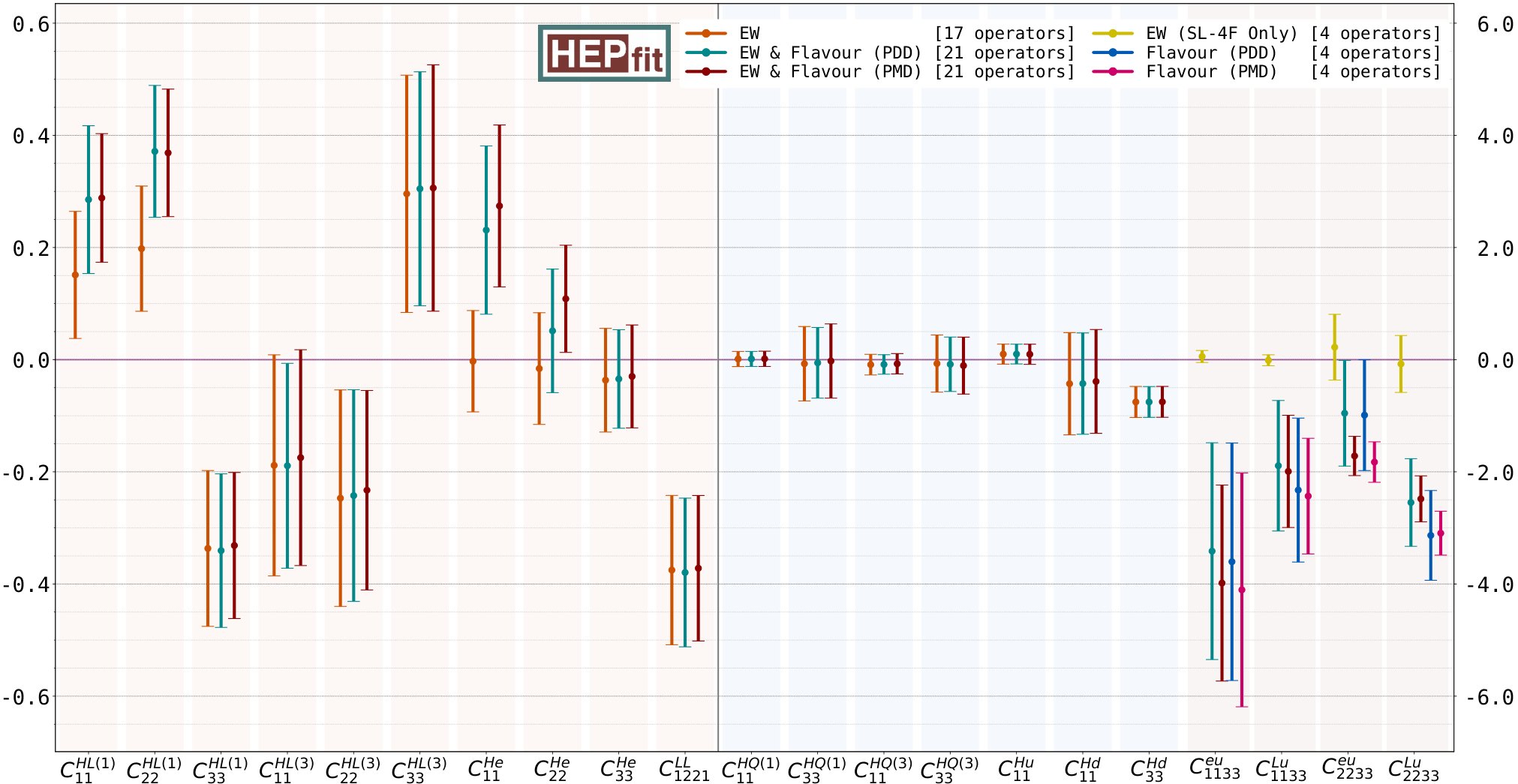
On the left side of figure 1, we show in orange the bounds from the EW fit on the Wilson coefficients of the operators with leptonic currents in terms of mean and standard deviation of the marginalized posterior probability density function. We observe compatibility with the SM within the 2 level. Note that EW data strongly correlate the operators under consideration among themselves, as can be seen in the correlation matrix presented in figure 2.

where away from the photon pole, are predicted to be unity at percent level Bordone:2016gaq.

In particular, the strong correlation between the operators with quarks and leptons is introduced by the non-negligible one-loop universal contribution of the operator to all the EW couplings, as anticipated at the end of section 4. With the direct bound on being relatively weak compared to the limits on the leptonic operators, such effects in the leptonic couplings can be sizable.
This leads to a relaxation of the naive bounds on , and that one would obtain in a tree-level analysis. To illustrate this, we present in appendix A a comparison with the results from such a tree level analysis of the EW fit. The results in figure 2 can then be compared to those in figure 8 where, as it is apparent, there is a substantial decoupling between the dimension-six operators made of Higgs doublets and quark bilinears from the leptonic ones.
The impact of these operators on the key observables for the present discussion is reported in figure 3. There, we collect mean and standard deviation on the shift in the coupling to light leptons (normalized to the corresponding SM value),and on the effect on in the dilepton-mass range GeV2:
| (10) |
Note that EW measurements tightly constrain NP effects modifying the EW gauge boson couplings to electrons, and also forbid deviations beyond the per-mille level in the case of couplings to muons. This translates into strong bounds on the Wilson coefficients . Hence, the one-loop contribution to from comes out to be tiny. We can then move our attention to the EW (SL-4F Only) scenario, reported in yellow in figure 1 and figure 3, and find a similar conclusion. Indeed, EW data once again strongly constrain the NP Wilson coefficients related to – the SL-4F operators – implying all the four NP Wilson coefficients to be compatible with 0. However, note that unlike the previous case, only contribute at one loop to and in eq. (10). Consequently, the resulting impact on flavour observables can be larger than the one in the EW scenario. As depicted in figure 3, however, there is still an overall tension between EWPO bounds (in yellow) and the experimental measurements of and (indicated by the shaded red boxes in the right side of the figure) at the 3 level.
To frame this tension from a different perspective, let us now focus on the set of flavour measurements as previously done in ref. Ciuchini:2019usw. In figure 1 we also show the constraints on the four Wilson coefficients of eq. (2) coming from data, in what we dubbed as the Flavour scenario. We present the PMD case, corresponding to an optimistic approach to QCD power corrections, in pink, while the more conservative PDD case is shown in blue. We observe that in both cases a muonic solution to anomalies stands out, with different from 0 at more than 3 in the PDD case, and at roughly 6 in the PMD one.
We stress that the difference between the results obtained in the PMD and in the PDD case is substantially driven by the angular analysis of . In particular, only within the PDD approach the fully left-handed solution to anomalies, , is favoured by data (signalled here by the Wilson coefficient of being compatible with 0 at 1, see the results in blue in figure 1). In addition, an electron resolution of anomalies is, once again, viable only within PDD Ciuchini:2017mik; Ciuchini:2019usw.
In the Flavour scenario one can also predict the induced shift in the -boson couplings according to eq. (7), and these are shown in figure 3. As can be seen, would receive large contributions at one loop from in correspondence to the one-loop MFV-like resolution of anomalies. Such contribution would be, however, now in tension with the results from EW precision tests. In particular, as a reflection of the main role played by in the Flavour fit to the four NP Wilson coefficients considered, shows the most important deviation from the SM value. Also, the prediction of becomes indirectly sensitive to the underlying treatment of hadronic uncertainties adopted for the study of data. Therefore, we observe that within the PMD approach, the inconsistency between what is needed to address anomalies and what is required by EW measurements is even more severe than the 3 established in the EW (SL-4F Only) scenario, and imprinted also in the Flavour fit with the PDD approach. In fact, we stress once again that adopting light-cone sum-rule results Khodjamirian:2010vf for the long-distant effects in decay, the tension between anomalies and EW data reaches the 6 level.
So, how do we reach a consensus between measurements and EWPO?
Succinctly, an obvious solution which satisfies these constraints is a class of models where anomalies are addressed at tree level and where modifications to -lepton-lepton vertices are at the same time suppressed. However, these models would not offer a solution to anomalies of the MFV type envisaged so far, namely they would rely on the existence of sizeable new sources of flavour violation. At this point, we would like to emphasize that a combined fit of EW and flavour observables offers a new insight into this matter: it highlights strong correlations between the dimension-six operators and as is evident from figure 4. This figure presents a pictorial representation of the correlations between the leptonic operators included in the different fits.
Apart from the fits introduced in the previous section, for illustration purposes we also show in figure 4 the correlations obtained in a variant of the fit including also the four-fermion operators , labelled as EW (including SL-4F operators). This is shown in the upper-right corner of the figure. As can be seen in that panel, and one could deduce from the relations in eq. (7), in a pure EW fit adding the four-fermion operators would simply introduce 4 flat directions. These are illustrated by the links connecting the () and () operators, corresponding to 100% anti-correlation. Such flat directions are lifted upon the introduction of the flavour measurements of and , as can be seen in the lower panels of figure 4 for the EW & Flavour fits. Even then, due again to relations in eq. (2) and (7) and the comparatively different precision of the EW and flavour measurements, sizable correlations remain.
In figure 1 the imprint of these correlations is a shift of central values and an increase on the bounds on the corresponding Wilson coefficients, with red and green bars representing the outcome of the fit in the EW & Flavour scenario within the PMD and PDD approaches, respectively. The interplay between and is evident when comparing the reported red and green bounds versus the orange EW constraints on , and the yellow ones for . Consequently, as clearly depicted in figure 3, looking at the red and green ranges reported for the EW & Flavour scenario, puzzles are solved with EW precision being respected. It is important to emphasize that, despite the significant correlation between quark and lepton operators introduced by the one-loop effects of , quark operators play no significant role in reconciling the EWPO constraints with the solution to anomalies. This will become clearer in the next section, but can be easily understood from the fact that, as mentioned before, quark and lepton constraints are somewhat uncorrelated in the tree-level EW fit, and the fact that the one-loop corrections effect induced by are flavour universal.
4.2 A minimal EFT picture
Finally, let us draw what would be the minimal picture for NP out of the general analysis obtained with the 21 operators considered in the EW & Flavour scenario. Indeed, a simpler picture will serve as a guideline for the UV models discussed in section 5. As mentioned before, given the hadronic uncertainties at hand, the most economic explanation addressing in particular anomalies resides in the NP contribution from the fully left-handed operator, . In the present context this operator is generated at one loop by , according to eq. (2).

Then, in figure 5 we show in orange the overall constraint from data on within the most conservative approach to long-distance effects, i.e. the PDD one. In particular, in the left (right) panel we report the constraint on the muonic (electronic) scenario. In the same figure, we highlight with the vertical gray band the bound derived from the full correlated set of EWPO on the same operator. From the comparison of the orange and gray single-operator bounds, the tension between flavour and EW measurements is manifest at the 3 level in the left panel of figure 5. It gets even more pronounced in the right panel due to the precise probe of NP that EW gauge-boson couplings to electrons provide. In the same figure 5, we also show with the horizontal gray band the result of the EWPO constraints applied this time on the NP contribution coming exclusively from the operator . Note that this operator would also contribute to at one loop, but the size needed would be and it is out of scale in the vertical axis of the plot.
Most importantly, in the same figure we display in (dashed) magenta the 1(2) contour where EW data are reconciled with the one-loop MFV explanation of anomalies when a combined fit of the NP contributions from these two operators is performed. Therefore, heavy BSM degrees of freedom that, once integrated out, generate sizeable contributions both to the Wilson coefficient of and of are the key aspect of this scenario that addresses anomalies without requiring sources of flavour violation beyond SM ones.
Finally, note that the role played here by could be shared, in part, with , depending on how much departure is actually required from the fully left-handed solution to anomalies. As already noted, this fact critically depends on the information stemming from Ciuchini:2019usw. On general grounds, to relieve the bounds from EWPO, the presence of would also necessitate sizeable NP effects from .
As a last comment of this section we would also like to highlight that in the class of models considered the prediction for the LUV observable is always close to the one for : any hint of NP coming from Hiller:2014ula; Hurth:2014vma; Hiller:2014yaa; Hiller:2017bzc would not be addressed within the NP models considered here, mainly involving the operators in eq. (2) and (2). In the following sections we will put our focus on the economic EFT scenario captured in figure 5 to build up simple UV scenarios realizing the EFT picture here delineated.
5 Directions for UV models
In this section we discuss how the lesson derived from the SMEFT picture illustrated, in particular, in figure 5, can be realized in a minimal extension of the SM. Here, we explicitly show how models involving a new gauge boson around the TeV scale provide the most economic example of the correlations advertised in the previous section. This can be achieved if we have a coupled both to top and lepton SM fields. These couplings can be obtained introducing vector-like top and muon/electron partners reasonably close to the EW scale Kamenik:2017tnu; Fox:2018ldq, making this class of models potentially interesting also from the point of view of naturalness in the Higgs sector. Finally, we will also briefly comment on possible alternative scenarios that can be obtained with leptoquarks.
5.1 Z′ with vector-like partners
Let us start with the baseline presented originally in ref. Kamenik:2017tnu. A simple extension of the SM, able to address anomalies, and that does not introduce any explicit new source of flavour violation, can be conceived as follows:
- •
The SM gauge group, , is extended by a new Abelian gauge group, , under which SM fields are neutral;
- •
There is a new complex scalar field that spontaneously breaks , giving a mass to the gauge boson equal to ;
- •
A coloured vector-like top partner, , properly charged under and can mix with the right-handed top-quark field via a Yukawa interaction with ;
- •
A vector-like muonic partner, , doublet of and charged under , can mix with the muonic doublet via another Yukawa coupling of ;
- •
The couplings controlling the kinetic-mixing term, , and the quadratic scalar mixing, , are set to be phenomenologically negligible.99 9 Using naive dimensional analysis, both kinetic and scalar quadratic mixing should appear beyond the tree level suppressed at least by a loop factor and the corresponding SM-partner rotation angles.
Then, the UV model is completely characterized by eight new parameters: the gauge coupling , the mass and quartic of the renormalizable potential of , the new Yukawa couplings , here taken to be real, and the vector-like mass-term parameters . In particular, the Lagrangian of the model contains the following terms:
| (11) |
that characterize the mixing pattern of SM fields and vector-like partners.1010 10 Note that upon an opposite charge assignment for the vector-like fermionic partners than the one implicitly assumed, one should replace in eq. (11) with . Symmetry breaking of is triggered by , that implies the following fermionic mixing patterns:
| top sector: | ||||
| muon sector: |
where () indicates the -component (-component) with weak isospin (-1/2). Using the determinant and trace of the squared mass matrices, one can easily show that the eigenvalues and must satisfy Kamenik:2017tnu:
| (20) | |||||
that in the decoupling limit clearly yield: , .
Defining for the top sector the rotation matrix from the interaction to the mass basis following the convention:
| (21) |
and doing similarly for the muonic sector, the mixing angles between SM fields, and , and their partner mass eigenstates, and , can be conveniently expressed in terms of the dimensionless ratios and :
| (22) | |||
In a perturbative expansion in , eq. (22) clearly shows that the mixing in the top sector proceeds mainly through , while in the muonic sector one has and very tiny .
Hence, for , the leading couplings of the boson to the SM fields correspond to right-handed tops and to left-handed muons as well as neutrinos according to:1111 11 In what follows, for we will have ; consequently, .
| (23) | |||||
| (24) |
with being non-negligible only at order . Consequently, integrating out the relevantly generates the operator with Wilson coefficient:
| (25) |
together with four-fermion operators built of or fields that can be potentially probed at collider and by experimental signatures like -trident production.
From eq. (25) it is clear that in order to have TeV-2 as highlighted in figure 5, one needs to rely on a relatively low symmetry-breaking scale TeV;1212 12 Note that even for masses as low as , for and , the interactions of do not alter the phenomenology discussed here since the largest -generated effects are still suppressed as . for TeV this implies 1. In figure 6 we show the region corresponding to the explanation of anomalies via eq. (25) in the parameter space , fixing the gauge coupling for a tentative gauge boson at the TeV scale and the VEV of the new scalar field set to GeV and GeV in the left and right panel, respectively. In the same plot, we re-interpret in our scenario the most relevant collider constraints originally identified in ref. Camargo-Molina:2018cwu.

For small values of , the measurement of neutrino-trident production performed in Mishra:1991bv is effective, and its constraint is reported at the 2 level with the orange vertical band. Under the reasonable assumption that the boson is mainly produced at tree level in association with the pair, in the blue region we show the 95% high- constraint stemming from the recasting of the search at ATLAS Aaboud:2017buh, while in cyan we report the expected constraint on the model from the 4-tops analysis of CMS Sirunyan:2017roi, see ref. Camargo-Molina:2018cwu for further details. From the same work, we also adopt the expected collider constraints for future projected luminosity corresponding to 300 fb-1, shown with dashed lines. Note that these projections become of fundamental importance when it comes to probe the interesting 1 region connected to anomalies. In particular, the right panel in figure 6 captures the benchmark for a promising discovery at the High-Luminosity LHC.
Finally, in the same figure, fixing the partner Yukawa coupling to values as reported in the two panels, we mark in gray the region corresponding to the bound on the mass of the vector-like partner expected from collider, taken to be TeV from the search at ATLAS in ref. Aaboud:2018uek, and TeV from the CMS analysis of ref. Sirunyan:2019ofn.
As already discussed, the scenario depicted in figure 6 remains viable under the lens of EW precision as long as we also have some heavy new dynamics yielding at the EW scale an imprint of consistently with the correlation obtained in the left panel of figure 5.
A simple way to obtain such NP contribution would be to consider the joint effect that the leptonic mixing of the vector-like partner would have together with the kinetic mixing of the , so far neglected. The - mixing could also originate from charging the new scalar field under both Abelian gauge groups, introducing a small misalignment with the standard hypercharge in the UV. However, the required mixing of the would end up mediating light-quark pair annihilation into muons: the typical size of the Wilson coefficient of this four-fermion operator would be , in net tension with the di-muon bound from ATLAS Aaboud:2017buh, probing NP scales as high as - TeV for (dimensionless) couplings. Hence, we rule out here this possibility.
Interestingly, it is still possible to generate without relying on the - mixing, but rather invoking the presence in the UV theory of additional new vector-like leptonic states Thomas:1998wy; delAguila:2008pw. These ones may be phenomenologically interesting in relation to the problem of the origin of neutrino masses as well as for the prediction of the anomalous magnetic moment Kannike:2011ng, and may give peculiar multi-lepton signatures at colliders Kumar:2015tna; Bhattiprolu:2019vdu.
In the most economic scenario, we may consider the presence in the UV theory of a pair of new vector-like muonic partners: a singlet of , , and a triplet of , , where in both cases the subscript denotes the hypercharge of the fermion. These fields would have their own mass terms controlled by the parameters , and interact with the SM doublet via the Yukawa couplings according to:
| (26) |
where we have reported the case of vector-like muonic partners with hypercharge . We assume the new Yukawa couplings to be real. Another possibility of interest may be the one of replacing in eq. (26) with the Higgs doublet, , and involve then the pair of vector-like partners with hypercharge .
Integrating out these vector-like states from the theory would generate contributions related to delAguila:2008pw; Kannike:2011ng of the form:
| (27) | |||||
Clearly, in order to have and negligible 1313 13 We have indeed verified that a scenario involving at the same time and would not alter what already highlighted in figure 5, with the best-fit value for turning out to be of ., one would need to rely on a tuning of the triplet Wilson coefficient with one of the contributions coming from the singlet vector-like muonic partner. However, once generated at the NP scale , we observe that the relation established between the triplet and singlet contributions to would be stable under the RG flow of the SMEFT.
A final comment is needed for the electron scenario reported in the right panel of figure 5, that involves opposite signs for the Wilson coefficients of and discussed so far. For the former, we note that the sign highlighted in the matching in eq. (25) follows from having assumed the same sign for the charge of the vector-like top and muon partners under . Hence, assuming the vector-like electron partner to have the opposite charge of the top-partner one would be sufficient to accomplish . (Of course, this would also imply a distinct use in eq. (11) of and couplings in the Yukawa terms of the vector-like partners involved to keep the theory invariant under .) For what concerns the generation of , according to eq. (27) one needs to correlate once again the contribution stemming from , or from , with the effect coming from a triplet, that now needs to be identified with , namely the triplet of hypercharge .
Eventually, we wish also to comment on the possible role of the operator, so far neglected in this discussion, but of potential relevance more in general. In fact, as mentioned earlier, the presence of would be particularly needed in the case where hadronic corrections entering in the amplitude of would be of the size originally estimated in Khodjamirian:2010vf. In that case, a solution to flavour anomalies would be preferred in the muonic channel with NP Wilson coefficient also substantially deviating from 0, as already discussed in section 4.1. Then, one would need to involve also the operator to relieve possible tensions with EW precision. In a general picture, the required NP effects from can be obtained integrating out heavy vector-like leptonic doublets.
5.2 Leptoquark scenarios
An alternative way to reproduce the minimal EFT scenario of figure 5 would be via leptoquarks (LQ), particles generically predicted in grand unified theories (GUTs) Pati:1974yy; PhysRevLett.32.438. Notoriously, LQ-induced dimension-six operators could be potentially dangerous as they would lead to proton decay at tree level, forcing to push their scale up to the GUT scale. However, the outcome may drastically change in models where the couplings of the LQs would be non-universal with respect to lepton and/or quark flavours. In such a case their mass could be much lower than what typically expected in GUTs and their signatures may actually be probed at present colliders. Interestingly, such LQs are candidates that could explain the lepton flavour universality violation – even at the loop level here considered Camargo-Molina:2018cwu; Coy:2019rfr – hinted in the recent LHCb and Belle data. However, this would imply generically a rather non-trivial flavour structure in the theory Becirevic:2017jtw. For a comprehensive survey of LQ models, see for instance Buchmuller:1986zs; delAguila:2010mx; Alonso:2015sja; Dorsner:2016wpm; deBlas:2017xtg.
Here, we limit ourselves to the case of toy models that specifically generate the operators of interest, namely and , for (electron) or (muon). In these peculiar LQ models we then assume that couplings between right-handed top quarks and light leptons are the only ones that actually matter for TeV phenomenology.
In table 1 we list the vector and scalar LQs that constitute the potential LQ candidates able to generate the solutions for anomalies at one loop under scrutiny.
| Vector LQ: | Comments | |
|---|---|---|
| not of interest | ||
| not of interest | ||
| generates | ||
| generates | ||
| Scalar LQ: | ||
| not of interest | ||
| not of interest | ||
| generates | ||
| generates |
Looking back at figure 5, from the table above we recognize as the most economic LQ scenario for the resolution of anomalies at one loop, the case of the vector LQ for LUV effects originating from electron couplings, and the scalar for the ones associated to muons. The interaction terms of interest are:
| (28) |
leading to the corresponding matching condition:
| (29) |
In figure 7 we report in (lighter) magenta the underlying 1(2) region where anomalies are addressed in concordance with the minimal EFT picture of figure 5. In the same plot, we also show a conservative estimate of the present LHC constraint on the mass of the LQ states considered, based on the dedicated collider study of ref. Angelescu:2018tyl.
We conclude noting that from the point of view of realizing the economic EFT result in figure 5, these leptoquark models should again be supplied by the combination of a singlet and a triplet muon/electron partners. Otherwise, in these models the leading contribution to would appear only at the loop level, in net distinction with the scenario, where the - mixing could be a priori exploited.
6 Summary
In this work we have revisited the analysis of anomalies looking for NP solutions that generate these FCNC processes at one loop and do not involve any new source of flavour violation beyond the SM ones. To this end, we have performed a broad analysis with dimension-six operators in the SMEFT, combining the experimental data on -physics with measurements of EWPO. The general outcome of our study is summarized in figure 1 and, supported with figure 3, shows that a resolution of anomalies of the MFV nature can be made fully compatible with EW precision.
From the SMEFT results derived we have then proceeded to identifying a minimal EFT scenario as captured in figure 5, that served as a simple guidance for SM UV completions. In this regard, we have explored in some detail the top-phillic and muon/electron-phillic , interesting for direct searches at collider as highlighted in figure 6. We have also commented on the viable leptoquark scenarios, collected in table 1. For both and leptoquark solutions we have found that additional contributions were necessary in order to maintain coupling measurements under control: in particular, we have shown that a correlated pair of vector-like leptons, a singlet and a triplet, can realize the minimal EFT scenario depicted on figure 5. We observe that the existence of these particles may be independently motivated by the heavy new dynamics underlying the origin of neutrino masses and/or by a tentative explanation of the anomaly Kannike:2011ng.
We conclude by noting that the measurement of decays at the scale of a few GeV is expected to reach a precision regime with the completion of the future runs at LHC and SuperKEKB. Hence, better measurements of the LUV observables and angular distributions of will be available in the next few years from Belle II Kou:2018nap and LHCb Bediaga:2018lhg. These will add a fundamental verification of the current interpretation of anomalies and of the direction in our search for NP signatures. Along these lines, should these signals of LUV persist, their interplay with EW precision measurements could be further tested at future colliders. In particular, circular colliders running at the pole, such as the FCC-ee Abada:2019lih; Abada:2019zxq or CEPC CEPCStudyGroup:2018ghi, could test deviations in the lepton universality of neutral weak currents with more than one order of magnitude improvement in precision compared to current data. At linear colliders, like the ILC Bambade:2019fyw or CLIC deBlas:2018mhx, where there is no proposed run at the pole, it would still be possible to obtain a significant improvement in the measurements of EWPO via radiative return to the Fujii:2019zll. Furthermore, the high-energy regime achievable at linear colliders would allow, after crossing the threshold, to directly test the effects of the interactions via . For the muon case, on the other hand, to test one would still need to rely on more complicated signals, such as , which would be in any case cleaner than at the LHC. (However, ideal optimal tests of these 4-fermion operators in 2-to-2 scattering processes would require a high-energy muon collider.) All of these could represent valuable additions from a “flavour” perspective in the interpretation of EW (and Higgs) measurements at these future machines within the EFT framework deBlas:2019rxi; deBlas:2019wgy.
Acknowledgements.
We warmly thank Ramona Gröber, Laura Reina and Luca Silvestrini for valuable feedback. The work of A.A. was in part supported by the MIUR contract 2017L5W2PT. J.B. acknowledges support by the UK Science and Technology Facilities Council (STFC) under grant ST/P001246/1. The work of M.V. is supported by the NSF Grant No. PHY-1915005. This research was supported in part through the Maxwell computational resources operated at DESY, Hamburg, Germany.Appendix A Discussions on EW fits

Here we revisit the constraints set by EWPO on the parameter space of the SMEFT. We make minimal flavour assumptions and include all quark and lepton operators described in the EW fit presented in section 3. Measurements of EWPO have been extensively studied in the literature Han:2004az; delAguila:2011zs; Ciuchini:2013pca; deBlas:2013gla; Falkowski:2014tna; Berthier:2015oma; Efrati:2015eaa; deBlas:2016nqo; deBlas:2017wmn; Ellis:2018gqa; Dawson:2019clf within the SMEFT framework. The purpose here is to provide further details on the correlation between quark and lepton sectors constrained by EWPO, illustrating some of the effects when going beyond the tree-level analysis.
The experimental inputs are the same considered for the EW fit in section 3, and include, in particular, the full set measurements taken at LEP/SLD at the pole, as well as the measurements of the boson obtained at LEP II, the Tevatron and the LHC (e.g. mass, width, branching ratios as well as the determination of at the LHC 1414 14 The extraction of could be, a priori, affected by other SMEFT effects entering in single-top production, e.g. 4-fermion operators. Such effects are neglected in our analysis. The only effect of this input in the EW fits in this paper is to lift a flat direction that would otherwise appear between and , had we excluded this measurement. Even with this input, these two coefficients are nearly correlated, as can be seen in figure 8.). For these fits we use the HEPfit package deBlas:2019okz as for the rest of the work.

We first consider the case of the EW fit at the tree level. In this case, the results of the fit reveal that while there is sizable correlation between the left-handed leptonic operators, as well as between the different quark operators, both sector are however decoupled to a good extent in the fit as can be seen from figure 8.
For the main fits presented in section 4, however, we also consider the leading logarithmically enhanced contributions at one-loop level via RG running. For our purposes, and considering the size of the bounds on the different operators from the EW fit, the most important contribution comes from . This induces an universal contribution that propagates into all EWPO. As a result of this, and similar to what was seen between the leptonic operators and the 4-fermion operators due to their interplay in eqs. (7), a non-trivial pattern of correlations between the lepton and quark operator sectors in the EW fit arises, as shown in figure 2. Similar to the change in the bounds on the leptonic operators in the EW+Flavour fit once we included the RG effects of the four-fermion operators, the bounds on the leptonic operators also relax in the EW fit once we include the RG effects from . This is shown in figure 9. However, unlike in the EW+Flavour fit, such effects do not induce a significant shift in the central values of the Wilson coefficients, which is simply due to the fact that the data selects to be centered around zero.
As can be seen in figure 9, the relaxation of the bounds can be in some cases rather dramatic, which brings about the question of what could be the impact of further effects not included in our analysis. We estimated that including the main RG effects for all the other operators in the EW fit amounts to changes of at most . One should also note that finite terms involving the Wilson coefficients of the quark coupling may become relevant at this point. As can be deduced from the full NLO results presented in Dawson:2019clf, these are not expected to significantly change the picture. In any case, the overall conclusions on this paper regarding the reconciliation between EW data and anomalies hold true.
References
- (1) A. Falkowski, F. Riva and A. Urbano, Higgs at last, JHEP 11 (2013) 111 [arXiv:1303.1812].
- (2) M. Ciuchini, E. Franco, S. Mishima and L. Silvestrini, Electroweak Precision Observables, New Physics and the Nature of a 126 GeV Higgs Boson, JHEP 08 (2013) 106 [arXiv:1306.4644].
- (3) A. Falkowski and F. Riva, Model-independent precision constraints on dimension-6 operators, JHEP 02 (2015) 039 [arXiv:1411.0669].
- (4) J. de Blas, M. Chala and J. Santiago, Renormalization Group Constraints on New Top Interactions from Electroweak Precision Data, JHEP 09 (2015) 189 [arXiv:1507.00757].
- (5) J. de Blas, M. Ciuchini, E. Franco, S. Mishima, M. Pierini, L. Reina and L. Silvestrini, Electroweak precision observables and Higgs-boson signal strengths in the Standard Model and beyond: present and future, JHEP 12 (2016) 135 [arXiv:1608.01509].
- (6) J. de Blas, M. Ciuchini, E. Franco, S. Mishima, M. Pierini, L. Reina and L. Silvestrini, The Global Electroweak and Higgs Fits in the LHC era, PoS EPS-HEP2017 (2017) 467 [arXiv:1710.05402].
- (7) J. Haller, A. Hoecker, R. Kogler, K. Mönig, T. Peiffer and J. Stelzer, Update of the global electroweak fit and constraints on two-Higgs-doublet models, Eur. Phys. J. C 78 (2018) 675 [arXiv:1803.01853].
- (8) J. Ellis, C. W. Murphy, V. Sanz and T. You, Updated Global SMEFT Fit to Higgs, Diboson and Electroweak Data, JHEP 06 (2018) 146 [arXiv:1803.03252].
- (9) J. Erler and M. Schott, Electroweak Precision Tests of the Standard Model after the Discovery of the Higgs Boson, Prog. Part. Nucl. Phys. 106 (2019) 68 [arXiv:1902.05142].
- (10) S. Dawson, S. Homiller and S. D. Lane, Putting SMEFT Fits to Work, arXiv:2007.01296.
- (11) B. Bhattacharya, A. Datta, D. London and S. Shivashankara, Simultaneous Explanation of the and Puzzles, Phys. Lett. B 742 (2015) 370 [arXiv:1412.7164].
- (12) F. Feruglio, P. Paradisi and A. Pattori, Revisiting Lepton Flavor Universality in B Decays, Phys. Rev. Lett. 118 (2017) 011801 [arXiv:1606.00524].
- (13) A. Celis, J. Fuentes-Martin, A. Vicente and J. Virto, Gauge-invariant implications of the LHCb measurements on lepton-flavor nonuniversality, Phys. Rev. D 96 (2017) 035026 [arXiv:1704.05672].
- (14) D. Buttazzo, A. Greljo, G. Isidori and D. Marzocca, B-physics anomalies: a guide to combined explanations, JHEP 11 (2017) 044 [arXiv:1706.07808].
- (15) J. Kumar, D. London and R. Watanabe, Combined Explanations of the and Anomalies: a General Model Analysis, Phys. Rev. D99 (2019) 015007 [arXiv:1806.07403].
- (16) M. Ciuchini, A. M. Coutinho, M. Fedele, E. Franco, A. Paul, L. Silvestrini and M. Valli, New Physics in confronts new data on Lepton Universality, Eur. Phys. J. C79 (2019) 719 [arXiv:1903.09632].
- (17) J. Aebischer, W. Altmannshofer, D. Guadagnoli, M. Reboud, P. Stangl and D. M. Straub, B-decay discrepancies after Moriond 2019, Eur. Phys. J. C80 (2020) 252 [arXiv:1903.10434].
- (18) C. Cornella, J. Fuentes-Martin and G. Isidori, Revisiting the vector leptoquark explanation of the B-physics anomalies, JHEP 07 (2019) 168 [arXiv:1903.11517].
- (19) LHCb collaboration, Test of lepton universality using decays, Phys. Rev. Lett. 113 (2014) 151601 [arXiv:1406.6482].
- (20) LHCb collaboration, Test of lepton universality with decays, JHEP 08 (2017) 055 [arXiv:1705.05802].
- (21) LHCb collaboration, Search for lepton-universality violation in decays, Phys. Rev. Lett. 122 (2019) 191801 [arXiv:1903.09252].
- (22) Belle collaboration, Test of lepton flavor universality in decays at Belle, arXiv:1904.02440.
- (23) G. Hiller and M. Schmaltz, and future physics beyond the standard model opportunities, Phys. Rev. D90 (2014) 054014 [arXiv:1408.1627].
- (24) G. Hiller and M. Schmaltz, Diagnosing lepton-nonuniversality in , JHEP 02 (2015) 055 [arXiv:1411.4773].
- (25) M. Bordone, G. Isidori and A. Pattori, On the Standard Model predictions for and , Eur. Phys. J. C 76 (2016) 440 [arXiv:1605.07633].
- (26) G. D’Amico, M. Nardecchia, P. Panci, F. Sannino, A. Strumia, R. Torre and A. Urbano, Flavour anomalies after the measurement, JHEP 09 (2017) 010 [arXiv:1704.05438].
- (27) L.-S. Geng, B. Grinstein, S. Jäger, J. Martin Camalich, X.-L. Ren and R.-X. Shi, Towards the discovery of new physics with lepton-universality ratios of decays, Phys. Rev. D 96 (2017) 093006 [arXiv:1704.05446].
- (28) B. Capdevila, A. Crivellin, S. Descotes-Genon, J. Matias and J. Virto, Patterns of New Physics in transitions in the light of recent data, JHEP 01 (2018) 093 [arXiv:1704.05340].
- (29) M. Ciuchini, A. M. Coutinho, M. Fedele, E. Franco, A. Paul, L. Silvestrini and M. Valli, On Flavourful Easter eggs for New Physics hunger and Lepton Flavour Universality violation, Eur. Phys. J. C77 (2017) 688 [arXiv:1704.05447].
- (30) G. Hiller and I. Nisandzic, and beyond the standard model, Phys. Rev. D 96 (2017) 035003 [arXiv:1704.05444].
- (31) A. K. Alok, A. Dighe, S. Gangal and D. Kumar, Continuing search for new physics in decays: two operators at a time, JHEP 06 (2019) 089 [arXiv:1903.09617].
- (32) M. Algueró, B. Capdevila, A. Crivellin, S. Descotes-Genon, P. Masjuan, J. Matias, M. Novoa et al., Emerging patterns of New Physics with and without Lepton Flavour Universal contributions, Eur. Phys. J. C 79 (2019) 714 [arXiv:1903.09578].
- (33) K. Kowalska, D. Kumar and E. M. Sessolo, Implications for new physics in transitions after recent measurements by Belle and LHCb, Eur. Phys. J. C 79 (2019) 840 [arXiv:1903.10932].
- (34) A. Arbey, T. Hurth, F. Mahmoudi, D. M. Santos and S. Neshatpour, Update on the bs anomalies, Phys. Rev. D 100 (2019) 015045 [arXiv:1904.08399].
- (35) A. Datta, J. Kumar and D. London, The anomalies and new physics in , Phys. Lett. B 797 (2019) 134858 [arXiv:1903.10086].
- (36) S. Descotes-Genon, J. Matias and J. Virto, Understanding the Anomaly, Phys. Rev. D88 (2013) 074002 [arXiv:1307.5683].
- (37) S. Descotes-Genon, L. Hofer, J. Matias and J. Virto, Global analysis of anomalies, JHEP 06 (2016) 092 [arXiv:1510.04239].
- (38) LHCb collaboration, Measurement of -averaged observables in the decay, arXiv:2003.04831.
- (39) A. Khodjamirian, T. Mannel, A. A. Pivovarov and Y. M. Wang, Charm-loop effect in and , JHEP 09 (2010) 089 [arXiv:1006.4945].
- (40) J. Lyon and R. Zwicky, Resonances gone topsy turvy - the charm of QCD or new physics in ?, arXiv:1406.0566.
- (41) V. Chobanova, T. Hurth, F. Mahmoudi, D. Martinez Santos and S. Neshatpour, Large hadronic power corrections or new physics in the rare decay ?, JHEP 07 (2017) 025 [arXiv:1702.02234].
- (42) T. Blake, U. Egede, P. Owen, K. A. Petridis and G. Pomery, An empirical model to determine the hadronic resonance contributions to transitions, Eur. Phys. J. C 78 (2018) 453 [arXiv:1709.03921].
- (43) C. Bobeth, M. Chrzaszcz, D. van Dyk and J. Virto, Long-distance effects in from analyticity, Eur. Phys. J. C 78 (2018) 451 [arXiv:1707.07305].
- (44) S. Jäger and J. Martin Camalich, Reassessing the discovery potential of the decays in the large-recoil region: SM challenges and BSM opportunities, Phys. Rev. D 93 (2016) 014028 [arXiv:1412.3183].
- (45) M. Ciuchini, M. Fedele, E. Franco, S. Mishima, A. Paul, L. Silvestrini and M. Valli, decays at large recoil in the Standard Model: a theoretical reappraisal, JHEP 06 (2016) 116 [arXiv:1512.07157].
- (46) A. Arbey, T. Hurth, F. Mahmoudi and S. Neshatpour, Hadronic and New Physics Contributions to Transitions, Phys. Rev. D 98 (2018) 095027 [arXiv:1806.02791].
- (47) M. Chrzaszcz, A. Mauri, N. Serra, R. Silva Coutinho and D. van Dyk, Prospects for disentangling long- and short-distance effects in the decays , JHEP 10 (2019) 236 [arXiv:1805.06378].
- (48) M. Ciuchini, A. M. Coutinho, M. Fedele, E. Franco, A. Paul, L. Silvestrini and M. Valli, Hadronic uncertainties in semileptonic decays, PoS BEAUTY2018 (2018) 044 [arXiv:1809.03789].
- (49) T. Hurth, F. Mahmoudi and S. Neshatpour, On the new LHCb angular analysis of : Hadronic effects or New Physics?, arXiv:2006.04213.
- (50) B. Capdevila, S. Descotes-Genon, J. Matias and J. Virto, Assessing lepton-flavour non-universality from angular analyses, JHEP 10 (2016) 075 [arXiv:1605.03156].
- (51) N. Serra, R. Silva Coutinho and D. van Dyk, Measuring the breaking of lepton flavor universality in , Phys. Rev. D 95 (2017) 035029 [arXiv:1610.08761].
- (52) Belle collaboration, Lepton-Flavor-Dependent Angular Analysis of , Phys. Rev. Lett. 118 (2017) 111801 [arXiv:1612.05014].
- (53) M. Algueró, B. Capdevila, S. Descotes-Genon, P. Masjuan and J. Matias, What and can tell us about New Physics in transitions?, JHEP 07 (2019) 096 [arXiv:1902.04900].
- (54) Belle-II collaboration, The Belle II Physics Book, PTEP 2019 (2019) 123C01 [arXiv:1808.10567].
- (55) LHCb collaboration, Search for the rare decays and , Phys. Rev. Lett. 124 (2020) 211802 [arXiv:2003.03999].
- (56) CMS collaboration, Measurement of the Branching Fraction and Search for with the CMS Experiment, Phys. Rev. Lett. 111 (2013) 101804 [arXiv:1307.5025].
- (57) LHCb collaboration, Measurement of the branching fraction and effective lifetime and search for decays, Phys. Rev. Lett. 118 (2017) 191801 [arXiv:1703.05747].
- (58) ATLAS collaboration, Study of the rare decays of and mesons into muon pairs using data collected during 2015 and 2016 with the ATLAS detector, JHEP 04 (2019) 098 [arXiv:1812.03017].
- (59) C. Bobeth, M. Gorbahn, T. Hermann, M. Misiak, E. Stamou and M. Steinhauser, in the Standard Model with Reduced Theoretical Uncertainty, Phys. Rev. Lett. 112 (2014) 101801 [arXiv:1311.0903].
- (60) A. Azatov, D. Bardhan, D. Ghosh, F. Sgarlata and E. Venturini, Anatomy of anomalies, JHEP 11 (2018) 187 [arXiv:1805.03209].
- (61) A. K. Alok, D. Kumar, S. Kumbhakar and S. Uma Sankar, Solutions to - in light of Belle 2019 data, Nucl. Phys. B 953 (2020) 114957 [arXiv:1903.10486].
- (62) C. Murgui, A. Peñuelas, M. Jung and A. Pich, Global fit to transitions, JHEP 09 (2019) 103 [arXiv:1904.09311].
- (63) R.-X. Shi, L.-S. Geng, B. Grinstein, S. Jäger and J. Martin Camalich, Revisiting the new-physics interpretation of the data, JHEP 12 (2019) 065 [arXiv:1905.08498].
- (64) BaBar collaboration, Measurement of an Excess of Decays and Implications for Charged Higgs Bosons, Phys. Rev. D 88 (2013) 072012 [arXiv:1303.0571].
- (65) Belle collaboration, Measurement of the branching ratio of relative to decays with hadronic tagging at Belle, Phys. Rev. D 92 (2015) 072014 [arXiv:1507.03233].
- (66) LHCb collaboration, Measurement of the ratio of the and branching fractions using three-prong -lepton decays, Phys. Rev. Lett. 120 (2018) 171802 [arXiv:1708.08856].
- (67) L. Di Luzio, A. Greljo and M. Nardecchia, Gauge leptoquark as the origin of B-physics anomalies, Phys. Rev. D 96 (2017) 115011 [arXiv:1708.08450].
- (68) L. Calibbi, A. Crivellin and T. Li, Model of vector leptoquarks in view of the -physics anomalies, Phys. Rev. D 98 (2018) 115002 [arXiv:1709.00692].
- (69) M. Bordone, C. Cornella, J. Fuentes-Martin and G. Isidori, A three-site gauge model for flavor hierarchies and flavor anomalies, Phys. Lett. B 779 (2018) 317 [arXiv:1712.01368].
- (70) R. Barbieri and A. Tesi, -decay anomalies in Pati-Salam SU(4), Eur. Phys. J. C 78 (2018) 193 [arXiv:1712.06844].
- (71) N. Assad, B. Fornal and B. Grinstein, Baryon Number and Lepton Universality Violation in Leptoquark and Diquark Models, Phys. Lett. B 777 (2018) 324 [arXiv:1708.06350].
- (72) J. Heeck and D. Teresi, Pati-Salam explanations of the B-meson anomalies, JHEP 12 (2018) 103 [arXiv:1808.07492].
- (73) B. Fornal, S. A. Gadam and B. Grinstein, Left-Right SU(4) Vector Leptoquark Model for Flavor Anomalies, Phys. Rev. D 99 (2019) 055025 [arXiv:1812.01603].
- (74) A. Crivellin, C. Greub, D. Müller and F. Saturnino, Importance of Loop Effects in Explaining the Accumulated Evidence for New Physics in B Decays with a Vector Leptoquark, Phys. Rev. Lett. 122 (2019) 011805 [arXiv:1807.02068].
- (75) A. Crivellin, D. Müller and F. Saturnino, Flavor Phenomenology of the Leptoquark Singlet-Triplet Model, JHEP 06 (2020) 020 [arXiv:1912.04224].
- (76) M. Bordone, O. Catà and T. Feldmann, Effective Theory Approach to New Physics with Flavour: General Framework and a Leptoquark Example, JHEP 01 (2020) 067 [arXiv:1910.02641].
- (77) UTfit collaboration, Model-independent constraints on operators and the scale of new physics, JHEP 03 (2008) 049 [arXiv:0707.0636].
- (78) L. Silvestrini and M. Valli, Model-independent Bounds on the Standard Model Effective Theory from Flavour Physics, Phys. Lett. B 799 (2019) 135062 [arXiv:1812.10913].
- (79) A. Greljo and D. Marzocca, High- dilepton tails and flavor physics, Eur. Phys. J. C77 (2017) 548 [arXiv:1704.09015].
- (80) M. J. Baker, J. Fuentes-Martín, G. Isidori and M. König, High- signatures in vector–leptoquark models, Eur. Phys. J. C79 (2019) 334 [arXiv:1901.10480].
- (81) L. Calibbi, A. Crivellin and T. Ota, Effective Field Theory Approach to , and with Third Generation Couplings, Phys. Rev. Lett. 115 (2015) 181801 [arXiv:1506.02661].
- (82) I. Doršner, S. Fajfer, A. Greljo, J. Kamenik and N. Košnik, Physics of leptoquarks in precision experiments and at particle colliders, Phys. Rept. 641 (2016) 1 [arXiv:1603.04993].
- (83) Belle collaboration, Measurement of the lepton polarization and in the decay , Phys. Rev. Lett. 118 (2017) 211801 [arXiv:1612.00529].
- (84) Belle collaboration, Measurement of and with a semileptonic tagging method, arXiv:1904.08794.
- (85) D. Bigi and P. Gambino, Revisiting , Phys. Rev. D 94 (2016) 094008 [arXiv:1606.08030].
- (86) F. U. Bernlochner, Z. Ligeti, M. Papucci and D. J. Robinson, Combined analysis of semileptonic decays to and : , , and new physics, Phys. Rev. D 95 (2017) 115008 [arXiv:1703.05330].
- (87) D. Bigi, P. Gambino and S. Schacht, , , and the Heavy Quark Symmetry relations between form factors, JHEP 11 (2017) 061 [arXiv:1707.09509].
- (88) S. Jaiswal, S. Nandi and S. K. Patra, Extraction of from and the Standard Model predictions of , JHEP 12 (2017) 060 [arXiv:1707.09977].
- (89) J. F. Kamenik, Y. Soreq and J. Zupan, Lepton flavor universality violation without new sources of quark flavor violation, Phys. Rev. D97 (2018) 035002 [arXiv:1704.06005].
- (90) P. J. Fox, I. Low and Y. Zhang, Top-philic forces at the LHC, JHEP 03 (2018) 074 [arXiv:1801.03505].
- (91) J. E. Camargo-Molina, A. Celis and D. A. Faroughy, Anomalies in Bottom from new physics in Top, Phys. Lett. B784 (2018) 284 [arXiv:1805.04917].
- (92) L. Di Luzio and M. Nardecchia, What is the scale of new physics behind the -flavour anomalies?, Eur. Phys. J. C 77 (2017) 536 [arXiv:1706.01868].
- (93) A. Buras, P. Gambino, M. Gorbahn, S. Jager and L. Silvestrini, Universal unitarity triangle and physics beyond the standard model, Phys. Lett. B 500 (2001) 161 [hep-ph/0007085].
- (94) G. D’Ambrosio, G. Giudice, G. Isidori and A. Strumia, Minimal flavor violation: An Effective field theory approach, Nucl. Phys. B 645 (2002) 155 [hep-ph/0207036].
- (95) A. L. Kagan, G. Perez, T. Volansky and J. Zupan, General Minimal Flavor Violation, Phys. Rev. D 80 (2009) 076002 [arXiv:0903.1794].
- (96) A. Efrati, A. Falkowski and Y. Soreq, Electroweak constraints on flavorful effective theories, JHEP 07 (2015) 018 [arXiv:1503.07872].
- (97) R. Coy, M. Frigerio, F. Mescia and O. Sumensari, New physics in transitions at one loop, Eur. Phys. J. C 80 (2020) 52 [arXiv:1909.08567].
- (98) E. E. Jenkins, A. V. Manohar and M. Trott, Renormalization Group Evolution of the Standard Model Dimension Six Operators I: Formalism and lambda Dependence, JHEP 10 (2013) 087 [arXiv:1308.2627].
- (99) E. E. Jenkins, A. V. Manohar and M. Trott, Renormalization Group Evolution of the Standard Model Dimension Six Operators II: Yukawa Dependence, JHEP 01 (2014) 035 [arXiv:1310.4838].
- (100) M. Ciuchini, M. Fedele, E. Franco, S. Mishima, A. Paul, L. Silvestrini and M. Valli, in the Standard Model: Elaborations and Interpretations, PoS ICHEP2016 (2016) 584 [arXiv:1611.04338].
- (101) M. Ciuchini, M. Fedele, E. Franco, S. Mishima, A. Paul, L. Silvestrini and M. Valli, Knowns and Unknowns in the Predictions for , Nucl. Part. Phys. Proc. 285-286 (2017) 45.
- (102) M. Ciuchini, A. M. Coutinho, M. Fedele, E. Franco, A. Paul, L. Silvestrini and M. Valli, On hadronic uncertainties polluting the New Physics hunt in transitions, Nucl. Part. Phys. Proc. 303-305 (2018) 8.
- (103) W. Buchmuller and D. Wyler, Effective Lagrangian Analysis of New Interactions and Flavor Conservation, Nucl. Phys. B 268 (1986) 621.
- (104) B. Grzadkowski, M. Iskrzynski, M. Misiak and J. Rosiek, Dimension-Six Terms in the Standard Model Lagrangian, JHEP 10 (2010) 085 [arXiv:1008.4884].
- (105) W. Altmannshofer, A. J. Buras, D. M. Straub and M. Wick, New strategies for New Physics search in , and decays, JHEP 04 (2009) 022 [arXiv:0902.0160].
- (106) A. J. Buras, J. Girrbach-Noe, C. Niehoff and D. M. Straub, decays in the Standard Model and beyond, JHEP 02 (2015) 184 [arXiv:1409.4557].
- (107) S. Descotes-Genon, S. Fajfer, J. F. Kamenik and M. Novoa-Brunet, Implications of Anomalies for Future Measurements of and , arXiv:2005.03734.
- (108) J. Aebischer, A. Crivellin, M. Fael and C. Greub, Matching of gauge invariant dimension-six operators for and transitions, JHEP 05 (2016) 037 [arXiv:1512.02830].
- (109) C. Bobeth, A. J. Buras, A. Celis and M. Jung, Yukawa enhancement of -mediated new physics in and processes, JHEP 07 (2017) 124 [arXiv:1703.04753].
- (110) G. Buchalla, A. J. Buras and M. E. Lautenbacher, Weak decays beyond leading logarithms, Rev. Mod. Phys. 68 (1996) 1125 [hep-ph/9512380].
- (111) A. J. Buras, Weak Hamiltonian, CP violation and rare decays, in Les Houches Summer School in Theoretical Physics, Session 68: Probing the Standard Model of Particle Interactions, pp. 281–539, 6, 1998, hep-ph/9806471.
- (112) L. Silvestrini, Effective Theories for Quark Flavour Physics, in Les Houches summer school: EFT in Particle Physics and Cosmology, 5, 2019, arXiv:1905.00798.
- (113) J. de Blas, J. Criado, M. Perez-Victoria and J. Santiago, Effective description of general extensions of the Standard Model: the complete tree-level dictionary, JHEP 03 (2018) 109 [arXiv:1711.10391].
- (114) J. de Blas, G. Durieux, C. Grojean, J. Gu and A. Paul, On the future of Higgs, electroweak and diboson measurements at lepton colliders, JHEP 12 (2019) 117 [arXiv:1907.04311].
- (115) B. Capdevila, A. Crivellin, C. A. Manzari and M. Montull, Explaining and the Cabbibo Angle Anomaly with a Vector Triplet, arXiv:2005.13542.
- (116) B. Belfatto, R. Beradze and Z. Berezhiani, The CKM unitarity problem: A trace of new physics at the TeV scale?, Eur. Phys. J. C 80 (2020) 149 [arXiv:1906.02714].
- (117) Y. Grossman, E. Passemar and S. Schacht, On the Statistical Treatment of the Cabibbo Angle Anomaly, arXiv:1911.07821.
- (118) J. de Blas et al., HEPfit: a Code for the Combination of Indirect and Direct Constraints on High Energy Physics Models, Eur. Phys. J. C 80 (2020) 456 [arXiv:1910.14012].
- (119) A. Caldwell, D. Kollár and K. Kröninger, BAT - The Bayesian analysis toolkit, Computer Physics Communications 180 (2009) 2197 [arXiv:0808.2552].
- (120) ALEPH, DELPHI, L3, OPAL, SLD, LEP Electroweak Working Group, SLD Electroweak Group, SLD Heavy Flavour Group collaboration, Precision electroweak measurements on the resonance, Phys. Rept. 427 (2006) 257 [hep-ex/0509008].
- (121) SLD collaboration, First direct measurement of the parity violating coupling of the Z0 to the s quark, Phys. Rev. Lett. 85 (2000) 5059 [hep-ex/0006019].
- (122) CDF, D0 collaboration, 2012 Update of the Combination of CDF and D0 Results for the Mass of the W Boson, arXiv:1204.0042.
- (123) ALEPH, DELPHI, L3, OPAL, LEP Electroweak collaboration, Electroweak Measurements in Electron-Positron Collisions at W-Boson-Pair Energies at LEP, Phys. Rept. 532 (2013) 119 [arXiv:1302.3415].
- (124) ATLAS collaboration, Measurement of the -boson mass in pp collisions at =7 TeV with the ATLAS detector, Eur. Phys. J. C 78 (2018) 110 [arXiv:1701.07240].
- (125) CMS collaboration, Measurement of the t-channel single-top-quark production cross section and of the CKM matrix element in pp collisions at = 8 TeV, JHEP 06 (2014) 090 [arXiv:1403.7366].
- (126) D0 collaboration, Measurement of and -light quark couplings using the forward-backward charge asymmetry in events with fb-1 at TeV, Phys. Rev. D 84 (2011) 012007 [arXiv:1104.4590].
- (127) ATLAS collaboration, Angular analysis of decays in collisions at TeV with the ATLAS detector, JHEP 10 (2018) 047 [arXiv:1805.04000].
- (128) CMS collaboration, Angular analysis of the decay from pp collisions at TeV, Phys. Lett. B753 (2016) 424 [arXiv:1507.08126].
- (129) CMS collaboration, Measurement of angular parameters from the decay in proton-proton collisions at 8 TeV, Phys. Lett. B781 (2018) 517 [arXiv:1710.02846].
- (130) LHCb collaboration, Angular analysis of the decay in the low-q2 region, JHEP 04 (2015) 064 [arXiv:1501.03038].
- (131) LHCb collaboration, Measurements of the S-wave fraction in decays and the differential branching fraction, JHEP 11 (2016) 047 [arXiv:1606.04731].
- (132) A. Paul and D. M. Straub, Constraints on new physics from radiative decays, JHEP 04 (2017) 027 [arXiv:1608.02556].
- (133) HFLAV collaboration, Averages of -hadron, -hadron, and -lepton properties as of 2018, arXiv:1909.12524.
- (134) LHCb collaboration, Differential branching fractions and isospin asymmetries of decays, JHEP 06 (2014) 133 [arXiv:1403.8044].
- (135) LHCb collaboration, Angular analysis and differential branching fraction of the decay , JHEP 09 (2015) 179 [arXiv:1506.08777].
- (136) LHCb collaboration, Measurement of the ratio of branching fractions and the direct CP asymmetry in , Nucl. Phys. B867 (2013) 1 [arXiv:1209.0313].
- (137) T. Hurth, F. Mahmoudi and S. Neshatpour, Global fits to data and signs for lepton non-universality, JHEP 12 (2014) 053 [arXiv:1410.4545].
- (138) CCFR collaboration, Neutrino tridents and W Z interference, Phys. Rev. Lett. 66 (1991) 3117.
- (139) ATLAS collaboration, Search for new high-mass phenomena in the dilepton final state using 36 fb-1 of proton-proton collision data at with the ATLAS detector, JHEP 10 (2017) 182 [arXiv:1707.02424].
- (140) CMS collaboration, Search for standard model production of four top quarks with same-sign and multilepton final states in proton–proton collisions at , Eur. Phys. J. C 78 (2018) 140 [arXiv:1710.10614].
- (141) ATLAS collaboration, Search for pair production of heavy vector-like quarks decaying into high- bosons and top quarks in the lepton-plus-jets final state in collisions at =13 TeV with the ATLAS detector, JHEP 08 (2018) 048 [arXiv:1806.01762].
- (142) CMS collaboration, Search for vector-like leptons in multilepton final states in proton-proton collisions at = 13 TeV, Phys. Rev. D 100 (2019) 052003 [arXiv:1905.10853].
- (143) S. D. Thomas and J. D. Wells, Phenomenology of Massive Vectorlike Doublet Leptons, Phys. Rev. Lett. 81 (1998) 34 [hep-ph/9804359].
- (144) F. del Aguila, J. de Blas and M. Perez-Victoria, Effects of new leptons in Electroweak Precision Data, Phys. Rev. D 78 (2008) 013010 [arXiv:0803.4008].
- (145) K. Kannike, M. Raidal, D. M. Straub and A. Strumia, Anthropic solution to the magnetic muon anomaly: the charged see-saw, JHEP 02 (2012) 106 [arXiv:1111.2551].
- (146) N. Kumar and S. P. Martin, Vectorlike Leptons at the Large Hadron Collider, Phys. Rev. D 92 (2015) 115018 [arXiv:1510.03456].
- (147) P. N. Bhattiprolu and S. P. Martin, Prospects for vectorlike leptons at future proton-proton colliders, Phys. Rev. D 100 (2019) 015033 [arXiv:1905.00498].
- (148) J. C. Pati and A. Salam, Lepton Number as the Fourth Color, Phys. Rev. D 10 (1974) 275.
- (149) H. Georgi and S. L. Glashow, Unity of all elementary-particle forces, Phys. Rev. Lett. 32 (1974) 438.
- (150) D. Bečirević and O. Sumensari, A leptoquark model to accommodate and , JHEP 08 (2017) 104 [arXiv:1704.05835].
- (151) W. Buchmuller, R. Ruckl and D. Wyler, Leptoquarks in Lepton - Quark Collisions, Phys. Lett. B 191 (1987) 442.
- (152) F. del Aguila, J. de Blas and M. Perez-Victoria, Electroweak Limits on General New Vector Bosons, JHEP 09 (2010) 033 [arXiv:1005.3998].
- (153) R. Alonso, B. Grinstein and J. Martin Camalich, Lepton universality violation and lepton flavor conservation in -meson decays, JHEP 10 (2015) 184 [arXiv:1505.05164].
- (154) A. Angelescu, D. Beˇcirević, D. Faroughy and O. Sumensari, Closing the window on single leptoquark solutions to the -physics anomalies, JHEP 10 (2018) 183 [arXiv:1808.08179].
- (155) LHCb collaboration, Physics case for an LHCb Upgrade II - Opportunities in flavour physics, and beyond, in the HL-LHC era, arXiv:1808.08865.
- (156) FCC collaboration, FCC Physics Opportunities: Future Circular Collider Conceptual Design Report Volume 1, Eur. Phys. J. C 79 (2019) 474.
- (157) FCC collaboration, FCC-ee: The Lepton Collider: Future Circular Collider Conceptual Design Report Volume 2, Eur. Phys. J. ST 228 (2019) 261.
- (158) CEPC Study Group collaboration, CEPC Conceptual Design Report: Volume 2 - Physics & Detector, arXiv:1811.10545.
- (159) P. Bambade et al., The International Linear Collider: A Global Project, arXiv:1903.01629.
- (160) R. Franceschini et al., The CLIC Potential for New Physics, arXiv:1812.02093.
- (161) LCC Physics Working Group collaboration, Tests of the Standard Model at the International Linear Collider, arXiv:1908.11299.
- (162) J. de Blas et al., Higgs Boson Studies at Future Particle Colliders, JHEP 01 (2020) 139 [arXiv:1905.03764].
- (163) Z. Han and W. Skiba, Effective theory analysis of precision electroweak data, Phys. Rev. D 71 (2005) 075009 [hep-ph/0412166].
- (164) F. del Aguila and J. de Blas, Electroweak constraints on new physics, Fortsch. Phys. 59 (2011) 1036 [arXiv:1105.6103].
- (165) J. de Blas, Electroweak limits on physics beyond the Standard Model, EPJ Web Conf. 60 (2013) 19008 [arXiv:1307.6173].
- (166) L. Berthier and M. Trott, Towards consistent Electroweak Precision Data constraints in the SMEFT, JHEP 05 (2015) 024 [arXiv:1502.02570].
- (167) J. de Blas, M. Ciuchini, E. Franco, S. Mishima, M. Pierini, L. Reina and L. Silvestrini, Electroweak precision constraints at present and future colliders, PoS ICHEP2016 (2017) 690 [arXiv:1611.05354].
- (168) S. Dawson and P. P. Giardino, Electroweak and QCD corrections to and pole observables in the standard model EFT, Phys. Rev. D 101 (2020) 013001 [arXiv:1909.02000].