跳到论文正文
W Papers独立论文阅读器 arXiv:2007.04204 论文正文 计算阅读时间 · 0%
引用这篇论文根据当前论文元数据生成,正式投稿前建议核对。


License: arXiv.org perpetual non-exclusive license
arXiv:2007.04204v1 [math.ST] 08 Jul 2020

pMAX Random Fields

Marta Ferreira Affiliation: Centro de Matemática da Universidade do Minho; Centro de Matemática Computacional e Estocástica da Universidade de Lisboa; Centro de Estatística e Aplicações da Universidade de Lisboa, Portugal, msferreira@math.uminho.pt    Ana Paula Martins Affiliation: Universidade da Beira Interior, Centro de Matemática e Aplicações (CMA-UBI), Avenida Marquês d’Avila e Bolama, 6200-001 Covilhã, Portugal, amartins@ubi.pt    Helena Ferreira Affiliation: Universidade da Beira Interior, Centro de Matemática e Aplicações (CMA-UBI), Avenida Marquês d’Avila e Bolama, 6200-001 Covilhã, Portugal, helenaf@ubi.pt
Abstract

The risk of occurrence of atypical phenomena is a cross-cutting concern in several areas, such as engineering, climatology, finance, actuarial, among others. Extreme value theory is the natural tool to approach this theme. Many of these random phenomena carry variables defined in time and space, usually modeled through random fields. Thus, the study of random fields in the context of extreme values becomes imperative and has been developed especially in the last decade. In this work, we propose a new random field, called pMAX, designed for modeling extremes. We analyze its dependence and pre-asymptotic dependence structure through the corresponding bivariate tail dependence coefficients. Estimators for the model parameters are obtained and their finite sample properties analyzed. Examples with simulations illustrate the results.

Keywords: extreme values, tail dependence coefficients, asymptotic independence, pMax

AMS 2000 Subject Classification: 60G70

1 Introduction

Modeling non-deterministic phenomena in a space-time context, such as precipitation values in a territory over a given period of time, can be done through random fields

{Y(x,t):x∈ℝ2,t∈ℝ+},\{Y(x,t):\,x\in\mathbb{R}^{2},\,t\in\mathbb{R}_{+}\},

where xx can be interpreted as the location and tt the instant at which the the random amount YY was recorded (see e.g. Buishand et al. [1] 2008, Hristopulos [5] 2020 and references therein).

Considering time discretization t∈ℕt\in\mathbb{N}, we can write the previous stochastic process as

{Y(x,n):x∈ℝ2,n∈ℕ}≡{Yn(x):x∈ℝ2,n∈ℕ}=⋃n≥1{Yn(x):x∈ℝ2}.\{Y(x,n):\,x\in\mathbb{R}^{2},\,n\in\mathbb{N}\}\equiv\{Y_{n}(x):\,x\in\mathbb{R}^{2},\,n\in\mathbb{N}\}=\bigcup_{n\geq 1}\{Y_{n}(x):\,x\in\mathbb{R}^{2}\}\,.

Thus, modeling through a sequence of random fields

{Yn​(x):x∈ℝ2}n≥1\{Y_{n}(x):\,x\in\mathbb{R}^{2}\}_{n\geq 1}

and studying their dependence and their finite marginal distributions is an approach for the space-time analysis of random phenomena.

In this work, we intend to analyze the simultaneous occurrence of extreme values for the random variables (r.v.’s) Yn​(x)Y_{n}(x) and Ym​(x′)Y_{m}(x^{\prime}), corresponding to any two locations xx and x′x^{\prime} and instants nn and mm, for a sequence of random fields {Yn​(x):x∈ℝ2}n≥1\{Y_{n}(x):\,x\in\mathbb{R}^{2}\}_{n\geq 1}, designated by pMAX fields. We say that a variable Yn​(x)Y_{n}(x) is pMAX, where pp is a reference to power, when it is of the form

Yn​(x)=Xn​(x)∨Zn​(x)1/α⁡(x),x∈ℝ2,\displaystyle Y_{n}(x)=X_{n}(x)\vee Z_{n}(x)^{1/\alpha(x)},\,x\in\mathbb{R}^{2}, (1)

where Xn​(x)X_{n}(x) and Zn​(x)Z_{n}(x) are r.v.’s and α⁡(x)>0\alpha(x)>0. In the literature there are models involving pMAX variables, as can be seen, for example, in Ferreira and Ferreira ([3] 2014), Heffernan et al. ([4] 2017) and references therein.

In the following section, we present the assumptions on the sequences of random fields {Xn​(x):x∈ℝ2}n≥1\{X_{n}(x):\,x\in\mathbb{R}^{2}\}_{n\geq 1}, {Zn​(x):x∈ℝ2}n≥1\{Z_{n}(x):\,x\in\mathbb{R}^{2}\}_{n\geq 1} and on the parameter function α:ℝ2→ℝ+\alpha:\mathbb{R}^{2}\to\mathbb{R}_{+}, considered along the paper. In Sections 3 and 4 we study the temporal, spatial and spatio-temporal dependence, as well as the tendency for oscillations in the high values. Events related to extremes of Yn​(x)Y_{n}(x), x∈ℝ2x\in\mathbb{R}^{2}, n≥1n\geq 1, will concern “exceedances of a real level yy” defined by {Yn(x)>y}\{Y_{n}(x)>y\}. The joint occurrence of high values for Yn​(x)Y_{n}(x) and Ym​(x′)Y_{m}(x^{\prime}) will be studied using bivariate tail dependence coefficients (Joe [6] 1997). The tendency for high values oscillations will be evaluated through functions of these coefficients. Section 4 addresses asymptotic independence in the sense of Ledford and Tawn ([7] 1996). This is a kind of weak or residual tail dependence vanishing at increasingly extreme quantiles and important for inferential purposes in order to avoid biased results. In section 5 we exemplify the results, strengthening the hypotheses for concrete models that we will simulate. Section 6 is devoted to the estimation of the model parameters α⁡(x)>0,\alpha(x)>0, x∈ℝ2.x\in\mathbb{R}^{2}.

2 Presenting the model

The pMAX random field that we propose is defined by (1), and satisfies conditions (i), (ii) and (iii) described below:

  • (i)

    {Xn​(x):x∈ℝ2}n≥1={𝐗n}n≥1\{X_{n}(x):\,x\in\mathbb{R}^{2}\}_{n\geq 1}=\{\mathbf{X}_{n}\}_{n\geq 1} is a stationary sequence of random fields with standard Fréchet marginals (i.e., P(Xn(x)≤z)=exp(−1/z)P(X_{n}(x)\leq z)=\exp(-1/z), z>0z>0);

  • (ii)

    {Zn​(x):x∈ℝ2}n≥1={𝐙n}n≥1\{Z_{n}(x):\,x\in\mathbb{R}^{2}\}_{n\geq 1}=\{\mathbf{Z}_{n}\}_{n\geq 1} is a sequence of independent and identically distributed (i.i.d.) random fields, with standard Fréchet marginals and independent of the previous sequence;

  • (iii)

    α⁡(x)\alpha(x), x∈ℝ2x\in\mathbb{R}^{2}, is a positive real valued function.

For any locations x,x′∈ℝ2x,x^{\prime}\in\mathbb{R}^{2}, z,z′>0z,z^{\prime}>0 and n,m≥1n,m\geq 1, we have:

  • P⁡(Yn​(x)≤z)=e−z−1​e−z−α⁡(x)P(Y_{n}(x)\leq z)=e^{-z^{-1}}e^{-z^{-\alpha(x)}},

  • P⁡(Yn​(x)≤z,Yn+m​(x′)≤z′)=P⁡(Xn​(x)≤z,Xn+m​(x′)≤z′)​e−z−α⁡(x)​e−z−α⁡(x′),P(Y_{n}(x)\leq z,Y_{n+m}(x^{\prime})\leq z^{\prime})=P(X_{n}(x)\leq z,X_{n+m}(x^{\prime})\leq z^{\prime})e^{-z^{-\alpha(x)}}e^{-z^{-\alpha(x^{\prime})}},

  • P⁡(Yn​(x)≤z,Yn​(x′)≤z′)=P⁡(Xn​(x)≤z,Xn​(x′)≤z′)​P​(Zn​(x)≤z,Zn​(x′)≤z′).P(Y_{n}(x)\leq z,Y_{n}(x^{\prime})\leq z^{\prime})=P(X_{n}(x)\leq z,X_{n}(x^{\prime})\leq z^{\prime})P(Z_{n}(x)\leq z,Z_{n}(x^{\prime})\leq z^{\prime}).

A sequence of pMAX random fields, {Yn​(x):x∈ℝ2}n≥1={𝐘n}n≥1\{Y_{n}(x):\,x\in\mathbb{R}^{2}\}_{n\geq 1}=\{\mathbf{Y}_{n}\}_{n\geq 1}, presents temporal and spatial dependence regulated by the function α\alpha and by the spatial and temporal dependence structure of {𝐗n}n≥1\{\mathbf{X}_{n}\}_{n\geq 1} and {𝐙n}n≥1\{\mathbf{Z}_{n}\}_{n\geq 1}, as we shall see.

3 Tail dependence

We describe the spatial and temporal dependence of the pMAX model through the tail dependence coefficient (Sibuya [9] 1960, Joe [6] 1997):

λ⁡(Yn+r​(x′)|Yn​(x))=limy→∞P⁡(Yn+r​(x′)>y|Yn​(x)>y),\displaystyle\lambda(Y_{n+r}(x^{\prime})|Y_{n}(x))=\displaystyle\lim_{y\to\infty}P(Y_{n+r}(x^{\prime})>y\ |\ Y_{n}(x)>y), (2)

with r≥0,r\geq 0, n≥1,n\geq 1, x,x′∈ℝ2.x,x^{\prime}\in\mathbb{R}^{2}.

It will be said that (Yn​(x),Yn+r​(x′))(Y_{n}(x),Y_{n+r}(x^{\prime})) is upper tail dependent when λ⁡(Yn+r​(x′)|Yn​(x))>0\lambda(Y_{n+r}(x^{\prime})|Y_{n}(x))>0 and upper tail independent if λ⁡(Yn+r​(x′)|Yn​(x))=0\lambda(Y_{n+r}(x^{\prime})|Y_{n}(x))=0.

When r>0r>0 and x=x′,x=x^{\prime}, λ⁡(Yn+r​(x)|Yn​(x))\lambda(Y_{n+r}(x)|Y_{n}(x)) summarizes the tail temporal dependence in location xx. If r=0r=0 and x≠x′x\not=x^{\prime}, then λ⁡(Yn​(x′)|Yn​(x))\lambda(Y_{n}(x^{\prime})|Y_{n}(x)) measures the tail spatial dependence between locations xx and x′x^{\prime}. When r>0r>0 and x≠x′,x\not=x^{\prime}, λ⁡(Yn+r​(x′)|Yn​(x))\lambda(Y_{n+r}(x^{\prime})|Y_{n}(x)) evaluates tail dependence in time and in space.

Proposition 3.1.

In a pMAX random field {𝐘n}n≥1\{\mathbf{Y}_{n}\}_{n\geq 1}, for r>0r>0, we have

λ⁡(Yn+r​(x′)|Yn​(x))={0,α(x)<112​λ​(Xn+r​(x′)|Xn​(x)),α(x)=1λ⁡(Xn+r​(x′)|Xn​(x)),α(x)>1,\displaystyle\lambda(Y_{n+r}(x^{\prime})|Y_{n}(x))=\left\{\begin{array}[]{ll}0&,\,\alpha(x)<1\\ \frac{1}{2}\lambda(X_{n+r}(x^{\prime})|X_{n}(x))&,\,\alpha(x)=1\\ \lambda(X_{n+r}(x^{\prime})|X_{n}(x))&,\,\alpha(x)>1\\ \end{array},\right.

and, if r=0r=0 and x≠x′x\not=x^{\prime}, then

λ⁡(Yn​(x′)|Yn​(x))={λ⁡(Zn​(x′)1/α⁡(x′)|Zn​(x)1/α⁡(x)),α(x)<112​(λ⁡(Xn​(x′)|Xn​(x))+λ⁡(Zn​(x′)1/α⁡(x′)|Zn​(x)1/α⁡(x))),α(x)=1λ⁡(Xn​(x′)|Xn​(x)),α(x)>1.\displaystyle\lambda(Y_{n}(x^{\prime})|Y_{n}(x))=\left\{\begin{array}[]{ll}\lambda(Z_{n}(x^{\prime})^{1/\alpha(x^{\prime})}|Z_{n}(x)^{1/\alpha(x)})&,\,\alpha(x)<1\\ \frac{1}{2}\left(\lambda(X_{n}(x^{\prime})|X_{n}(x))+\lambda(Z_{n}(x^{\prime})^{1/\alpha(x^{\prime})}|Z_{n}(x)^{1/\alpha(x)})\right)&,\,\alpha(x)=1\\ \lambda(X_{n}(x^{\prime})|X_{n}(x))&,\,\alpha(x)>1\\ \end{array}.\right.
Proof.

Observe that

P⁡(Yn+r​(x′)>y|Yn​(x)>y)=1−P⁡(Yn+r​(x′)≤y)−P⁡(Yn​(x)≤y)+P⁡(Yn​(x)≤y,Yn+r​(x′)≤y)1−P⁡(Yn​(x)≤y)\displaystyle P(Y_{n+r}(x^{\prime})>y\ |\ Y_{n}(x)>y)=\frac{1-P(Y_{n+r}(x^{\prime})\leq y)-P(Y_{n}(x)\leq y)+P(Y_{n}(x)\leq y,Y_{n+r}(x^{\prime})\leq y)}{1-P(Y_{n}(x)\leq y)}
=1−e−y−1−y−α⁡(x′)−P⁡(Xn​(x)≤y,Xn+r​(x′)≤y)​P​(Zn​(x)≤yα⁡(x),Zn+r​(x′)≤yα⁡(x′))1−e−y−1−y−α⁡(x)\displaystyle=1-\frac{e^{-y^{-1}-y^{-\alpha(x^{\prime})}}-P(X_{n}(x)\leq y,X_{n+r}(x^{\prime})\leq y)P(Z_{n}(x)\leq y^{\alpha(x)},Z_{n+r}(x^{\prime})\leq y^{\alpha(x^{\prime})})}{1-e^{-y^{-1}-y^{-\alpha(x)}}}
=1−e−y−1−y−α⁡(x′)−[P⁡(Xn+r​(x′)≤y)−P⁡(Xn​(x)>y,Xn+r​(x′)≤y)]​P​(Zn​(x)≤yα⁡(x),Zn+r​(x′)≤yα⁡(x′))1−e−y−1−y−α⁡(x)\displaystyle=1-\frac{e^{-y^{-1}-y^{-\alpha(x^{\prime})}}-\left[P(X_{n+r}(x^{\prime})\leq y)-P(X_{n}(x)>y,X_{n+r}(x^{\prime})\leq y)\right]P(Z_{n}(x)\leq y^{\alpha(x)},Z_{n+r}(x^{\prime})\leq y^{\alpha(x^{\prime})})}{1-e^{-y^{-1}-y^{-\alpha(x)}}}
=1−e−y−1−y−α⁡(x′)​1−P⁡(Zn​(x)≤yα⁡(x),Zn+r​(x′)≤yα⁡(x′))e−y−α⁡(x′)1−e−y−1−y−α⁡(x)\displaystyle=1-e^{-y^{-1}-y^{-\alpha(x^{\prime})}}\frac{1-\frac{P(Z_{n}(x)\leq y^{\alpha(x)},Z_{n+r}(x^{\prime})\leq y^{\alpha(x^{\prime})})}{e^{-y^{-\alpha(x^{\prime})}}}}{1-e^{-y^{-1}-y^{-\alpha(x)}}}
−P⁡(Xn+r​(x′)≤y|Xn​(x)>y)​1−e−y−11−e−y−1−y−α⁡(x)​P​(Zn​(x)≤yα⁡(x),Zn+r​(x′)≤yα⁡(x′)),\displaystyle\ \ \ -P(X_{n+r}(x^{\prime})\leq y\ |\ X_{n}(x)>y)\frac{1-e^{-y^{-1}}}{1-e^{-y^{-1}-y^{-\alpha(x)}}}P(Z_{n}(x)\leq y^{\alpha(x)},Z_{n+r}(x^{\prime})\leq y^{\alpha(x^{\prime})}),

where we have

limy→∞P⁡(Xn+r​(x′)≤y|Xn​(x)>y)​1−e−y−11−e−y−1−y−α⁡(x)​P​(Zn​(x)≤yα⁡(x),Zn+r​(x′)≤yα⁡(x′))\displaystyle\hskip-113.81102pt\lim_{y\to\infty}P(X_{n+r}(x^{\prime})\leq y\ |\ X_{n}(x)>y)\frac{1-e^{-y^{-1}}}{1-e^{-y^{-1}-y^{-\alpha(x)}}}P(Z_{n}(x)\leq y^{\alpha(x)},Z_{n+r}(x^{\prime})\leq y^{\alpha(x^{\prime})})
={0,α(x)<112​(1−λ⁡(Xn+r​(x′)|Xn​(x))),α(x)=11−λ⁡(Xn+r​(x′)|Xn​(x)),α(x)>1.\displaystyle\hskip-85.35826pt=\left\{\begin{array}[]{ll}0&,\,\alpha(x)<1\\ \frac{1}{2}(1-\lambda(X_{n+r}(x^{\prime})|X_{n}(x)))&,\,\alpha(x)=1\\ 1-\lambda(X_{n+r}(x^{\prime})|X_{n}(x))&,\,\alpha(x)>1\end{array}.\right.

If r>0r>0 then Zn​(x)Z_{n}(x) and Zn+r​(x′)Z_{n+r}(x^{\prime}) are independent and

limy→∞1−P⁡(Zn​(x)≤yα⁡(x),Zn+r​(x′)≤yα⁡(x′))e−y−α⁡(x′)1−e−y−1−y−α⁡(x)=limy→∞1−e−y−α⁡(x)1−e−y−1−y−α⁡(x)={1,α(x)<112,α(x)=10,α(x)>1.\lim_{y\to\infty}\frac{1-\frac{P(Z_{n}(x)\leq y^{\alpha(x)},Z_{n+r}(x^{\prime})\leq y^{\alpha(x^{\prime})})}{e^{-y^{-\alpha(x^{\prime})}}}}{1-e^{-y^{-1}-y^{-\alpha(x)}}}=\displaystyle\lim_{y\to\infty}\frac{1-e^{-y^{-\alpha(x)}}}{1-e^{-y^{-1}-y^{-\alpha(x)}}}=\left\{\begin{array}[]{ll}1&,\,\alpha(x)<1\\ \frac{1}{2}&,\,\alpha(x)=1\\ 0&,\,\alpha(x)>1\\ \end{array}.\right.

If r=0r=0 and x≠x′,x\not=x^{\prime}, then

limy→∞e−y−1−y−α⁡(x′)​1−P⁡(Zn​(x)≤yα⁡(x),Zn+r​(x′)≤yα⁡(x′))e−y−α⁡(x′)1−e−y−1−y−α⁡(x)\displaystyle\hskip-28.45274pt\lim_{y\to\infty}e^{-y^{-1}-y^{-\alpha(x^{\prime})}}\frac{1-\frac{P(Z_{n}(x)\leq y^{\alpha(x)},Z_{n+r}(x^{\prime})\leq y^{\alpha(x^{\prime})})}{e^{-y^{-\alpha(x^{\prime})}}}}{1-e^{-y^{-1}-y^{-\alpha(x)}}}
=limy→∞e−y−1−y−α⁡(x′)​1−P⁡(Zn+r​(x′)≤yα⁡(x′))−P⁡(Zn​(x)>yα⁡(x),Zn+r​(x′)≤yα⁡(x′))e−y−α⁡(x′)1−e−y−1−y−α⁡(x)\displaystyle=\lim_{y\to\infty}e^{-y^{-1}-y^{-\alpha(x^{\prime})}}\frac{1-\frac{P(Z_{n+r}(x^{\prime})\leq y^{\alpha(x^{\prime})})-P(Z_{n}(x)>y^{\alpha(x)},Z_{n+r}(x^{\prime})\leq y^{\alpha(x^{\prime})})}{e^{-y^{-\alpha(x^{\prime})}}}}{1-e^{-y^{-1}-y^{-\alpha(x)}}}
=P⁡(Zn+r​(x′)≤yα⁡(x′)|Zn​(x)>yα⁡(x))​(1−e−y−α⁡(x))1−e−y−1−y−α⁡(x)​e−y−1\displaystyle=\frac{P(Z_{n+r}(x^{\prime})\leq y^{\alpha(x^{\prime})}|Z_{n}(x)>y^{\alpha(x)})(1-e^{-y^{-\alpha(x)}})}{1-e^{-y^{-1}-y^{-\alpha(x)}}}e^{-y^{-1}}
={1−λ⁡(Zn​(x′)1/α⁡(x′)|Zn​(x)1/α⁡(x)),α(x)<112​(1−λ⁡(Zn​(x′)1/α⁡(x′)|Zn​(x)1/α⁡(x))),α(x)=10,α(x)>1.\displaystyle=\left\{\begin{array}[]{ll}1-\lambda(Z_{n}(x^{\prime})^{1/\alpha(x^{\prime})}|Z_{n}(x)^{1/\alpha(x)})&,\,\alpha(x)<1\\ \frac{1}{2}(1-\lambda(Z_{n}(x^{\prime})^{1/\alpha(x^{\prime})}|Z_{n}(x)^{1/\alpha(x)}))&,\,\alpha(x)=1\\ 0&,\,\alpha(x)>1\end{array}.\right.

∎

The previous result shows that the pMAX random field {𝐘n}n≥1\{\mathbf{Y}_{n}\}_{n\geq 1} is temporal or spatial-temporal upper tail independent when α⁡(x)<1,\alpha(x)<1, whereas upper tail dependence is regulated by the upper tail dependence of {𝐗n}n≥1.\{\mathbf{X}_{n}\}_{n\geq 1}. On the other hand, spatial upper tail dependence is regulated by the spatial dependence structure of {𝐗n}n≥1\{\mathbf{X}_{n}\}_{n\geq 1} and {𝐙n}n≥1.\{\mathbf{Z}_{n}\}_{n\geq 1}.

The case r>0r>0 above was already stated in Ferreira and Ferreira ([3] 2014; Proposition 2.5).

4 Pre-asymptotic dependence

Previously we have seen that tail dependence can be assessed through coefficient λ⁡(Yn+r​(x′)|Yn​(x))\lambda(Y_{n+r}(x^{\prime})|Y_{n}(x)), where a unit value means total dependence and a null value corresponds to tail independence. In the latter case, there may be a residual or pre-asymptotic dependence captured by the velocity of convergence of the limit in (2) towards zero. More precisely, if

P(Xn+r(x′)>y|Xn(x)>y)∼y−1/η(x′|x)(X,r)−1ℒ(x′|x)(X,r)(y)\displaystyle P(X_{n+r}(x^{\prime})>y\ |\ X_{n}(x)>y)\sim y^{-1/\eta_{(x^{\prime}|x)}^{(X,r)}-1}\mathcal{L}_{(x^{\prime}|x)}^{(X,r)}(y) (11)

as y→∞y\to\infty, where function ℒ(x′|x)(X,r)​(y)\mathcal{L}_{(x^{\prime}|x)}^{(X,r)}(y) is slow varying (ℒ⁡(y)\mathcal{L}(y) is a slow varying function if ℒ:ℝ+→ℝ\mathcal{L}:\mathbb{R}^{+}\to\mathbb{R} and ℒ⁡(t​y)/ℒ⁡(y)→1\mathcal{L}(ty)/\mathcal{L}(y)\to 1, as y→∞y\to\infty, t>0t>0), we say that η(x′|x)(X,r)∈(0,1]\eta_{(x^{\prime}|x)}^{(X,r)}\in(0,1] is a residual tail dependence coefficient usually denoted in literature as Ledford and Tawn tail dependence coefficient (see, e.g., Ledford and Tawn [7] 1996, Heffernan et al. [4] 2007, Ferreira and Ferreira [3] 2014 and references therein). Notation a⁡(y)∼b⁡(y)a(y)\sim b(y) in (11) stands for a⁡(y)/b⁡(y)→1a(y)/b(y)\to 1, as y→∞y\to\infty. Observe that η(x′|x)(X,r)\eta_{(x^{\prime}|x)}^{(X,r)} is a space-time measure if r>0r>0 and x≠x′x\not=x^{\prime}, a temporal measure if r>0r>0 and x=x′x=x^{\prime} and a spatial measure if r=0r=0 and x≠x′x\not=x^{\prime} (we denote η(x′|x)(X)≡η(x′|x)(X,0)\eta_{(x^{\prime}|x)}^{(X)}\equiv\eta_{(x^{\prime}|x)}^{(X,0)}). Observe that tail dependence (λ>0\lambda>0) corresponds to η=1\eta=1 and η<1\eta<1 means asymptotic tail independence. Under exact independence we have η=1/2\eta=1/2. A classical example is assigned to Gaussian random pairs with correlation coefficient ρ\rho, where η=(1+ρ)/2\eta=(1+\rho)/2.

Proposition 4.1.

In a pMAX random field satisfying (11) with r>0r>0, we have

η(x′|x)(Y,r)={α⁡(x)​max⁡(η(x′|x)(X,r),11+min⁡(α⁡(x′),1)),α(x)<1max⁡(η(x′|x)(X),11+α⁡(x),11+α⁡(x′)),α(x)≥1.\eta_{(x^{\prime}|x)}^{(Y,r)}=\left\{\begin{array}[]{ll}\alpha(x)\max\left(\eta_{(x^{\prime}|x)}^{(X,r)},\frac{1}{1+\min(\alpha(x^{\prime}),1)}\right)&,\,\alpha(x)<1\\ \\ \max\left(\eta_{(x^{\prime}|x)}^{(X)},\frac{1}{1+\alpha(x)},\frac{1}{1+\alpha(x^{\prime})}\right)&,\,\alpha(x)\geq 1\end{array}.\right.

If r=0r=0 and, in addition,

P(Zn(x′)1/α⁡(x′)>y|Zn(x)1/α⁡(x)>y)∼y−1/η(α⁡(x′)|α⁡(x))(Z)−1ℒ(α⁡(x′),α⁡(x))(Z)(y)\displaystyle P(Z_{n}(x^{\prime})^{1/\alpha(x^{\prime})}>y\ |\ Z_{n}(x)^{1/\alpha(x)}>y)\sim y^{-1/\eta_{(\alpha(x^{\prime})|\alpha(x))}^{(Z)}-1}\mathcal{L}_{(\alpha(x^{\prime}),\alpha(x))}^{(Z)}(y) (12)

holds, as y→∞y\to\infty, where ℒ(α⁡(x′),α⁡(x))(Z)​(y)\mathcal{L}_{(\alpha(x^{\prime}),\alpha(x))}^{(Z)}(y) is a slowly varying function and η(α⁡(x′)|α⁡(x))(Z)∈(0,1]\eta_{(\alpha(x^{\prime})|\alpha(x))}^{(Z)}\in(0,1], then

η(x′|x)(Y)=min⁡(1,α⁡(x))​max⁡(η(x′|x)(X),η(α⁡(x′)|α⁡(x))(Z),11+α⁡(x),11+α⁡(x′)).\eta_{(x^{\prime}|x)}^{(Y)}=\min\left(1,\alpha(x)\right)\max\left(\eta_{(x^{\prime}|x)}^{(X)},\eta_{(\alpha(x^{\prime})|\alpha(x))}^{(Z)},\frac{1}{1+\alpha(x)},\frac{1}{1+\alpha(x^{\prime})}\right).
Proof.

Observe that

P⁡(Yn+r​(x′)>y,Yn​(x)>y)\displaystyle P(Y_{n+r}(x^{\prime})>y,Y_{n}(x)>y)
=\displaystyle= P⁡(Xn+r​(x′)>y,Xn​(x)>y)​(1−P⁡(Zn+r​(x′)>yα⁡(x′))−P⁡(Zn​(x)>yα⁡(x)))\displaystyle P(X_{n+r}(x^{\prime})>y,X_{n}(x)>y)\left(1-P(Z_{n+r}(x^{\prime})>y^{\alpha(x^{\prime})})-P(Z_{n}(x)>y^{\alpha(x)})\right)
+P⁡(Zn+r​(x′)>yα⁡(x′),Zn​(x)>yα⁡(x))​(1−P⁡(Xn+r​(x′)>y)−P⁡(Xn​(x)>y))\displaystyle+\ P(Z_{n+r}(x^{\prime})>y^{\alpha(x^{\prime})},Z_{n}(x)>y^{\alpha(x)})\left(1-P(X_{n+r}(x^{\prime})>y)-P(X_{n}(x)>y)\right)
+P⁡(Xn+r​(x′)>y,Xn​(x)>y)​P​(Zn+r​(x′)>yα⁡(x′),Zn​(x)>yα⁡(x))\displaystyle+\ P(X_{n+r}(x^{\prime})>y,X_{n}(x)>y)P(Z_{n+r}(x^{\prime})>y^{\alpha(x^{\prime})},Z_{n}(x)>y^{\alpha(x)})
+P⁡(Xn​(x)>y)​P​(Zn+r​(x′)>yα⁡(x′))+P⁡(Xn+r​(x′)>y)​P​(Zn​(x)>yα⁡(x))\displaystyle+\ P(X_{n}(x)>y)P(Z_{n+r}(x^{\prime})>y^{\alpha(x^{\prime})})+P(X_{n+r}(x^{\prime})>y)P(Z_{n}(x)>y^{\alpha(x)})

and thus, as y→∞y\to\infty,

P⁡(Yn+r​(x′)>y,Yn​(x)>y)\displaystyle P(Y_{n+r}(x^{\prime})>y,Y_{n}(x)>y)
∼\displaystyle\sim P⁡(Xn+r​(x′)>y,Xn​(x)>y)+P⁡(Zn+r​(x′)>yα⁡(x′),Zn​(x)>yα⁡(x))+y−1​(y−α⁡(x′)+y−α⁡(x)).\displaystyle P(X_{n+r}(x^{\prime})>y,X_{n}(x)>y)+P(Z_{n+r}(x^{\prime})>y^{\alpha(x^{\prime})},Z_{n}(x)>y^{\alpha(x)})+y^{-1}\left(y^{-\alpha(x^{\prime})}+y^{-\alpha(x)}\right).

If r>0r>0, under condition (11), we have

P(Yn+r(x′)>y,Yn(x)>y)∼y−1/η(x′|x)(X)ℒ(x′|x)(X)(y)+y−α⁡(x′)−α⁡(x)+y−1(y−α⁡(x′)+y−α⁡(x)).P(Y_{n+r}(x^{\prime})>y,Y_{n}(x)>y)\sim y^{-1/\eta_{(x^{\prime}|x)}^{(X)}}\mathcal{L}_{(x^{\prime}|x)}^{(X)}(y)+y^{-\alpha(x^{\prime})-\alpha(x)}+y^{-1}\left(y^{-\alpha(x^{\prime})}+y^{-\alpha(x)}\right).

and therefore

P⁡(Yn+r​(x′)>y,Yn​(x)>y)P​(Yn​(x)>y)1/η(x′|x)(Y)∼y−1/η(x′|x)(X)ℒ(x′|x)(X)(y)+y−α⁡(x′)−α⁡(x)+y−1−α⁡(x′)+y−1−α⁡(x)(y−1+y−α⁡(x))1/η(x′|x)(Y).\frac{P(Y_{n+r}(x^{\prime})>y,Y_{n}(x)>y)}{P(Y_{n}(x)>y)^{1/\eta_{(x^{\prime}|x)}^{(Y)}}}\sim\displaystyle\frac{y^{-1/\eta_{(x^{\prime}|x)}^{(X)}}\mathcal{L}_{(x^{\prime}|x)}^{(X)}(y)+y^{-\alpha(x^{\prime})-\alpha(x)}+y^{-1-\alpha(x^{\prime})}+y^{-1-\alpha(x)}}{\left(y^{-1}+y^{-\alpha(x)}\right)^{1/\eta_{(x^{\prime}|x)}^{(Y)}}}.

If r=0r=0, just observe that, by (11) and (12), we have

P⁡(Yn​(x′)>y,Yn​(x)>y)\displaystyle P(Y_{n}(x^{\prime})>y,Y_{n}(x)>y)
∼\displaystyle\sim y−1/η(x′|x)(X)ℒ(x′|x)(X)(y)+y−1/η(α⁡(x′)|α⁡(x))(Z)ℒ(α⁡(x′)|α⁡(x))(Z)(y)+y−1(y−α⁡(x′)+y−α⁡(x)).\displaystyle y^{-1/\eta_{(x^{\prime}|x)}^{(X)}}\mathcal{L}_{(x^{\prime}|x)}^{(X)}(y)+y^{-1/\eta_{(\alpha(x^{\prime})|\alpha(x))}^{(Z)}}\mathcal{L}_{(\alpha(x^{\prime})|\alpha(x))}^{(Z)}(y)+y^{-1}\left(y^{-\alpha(x^{\prime})}+y^{-\alpha(x)}\right).

∎

The case r>0r>0 in the previous result was already derived in Ferreira and Ferreira ([3] 2014; Proposition 2.6)

5 Examples

For the pMAX model defined in (1) we shall now consider particular cases of {Xn​(x),x∈ℝ2}n≥1\{X_{n}(x),x\in\mathbb{R}^{2}\}_{n\geq 1} and {Zn​(x),x∈ℝ2}n≥1\{Z_{n}(x),x\in\mathbb{R}^{2}\}_{n\geq 1} to illustrate the several types of dependence captured by the previously presented coefficients. {Xn​(x),x∈ℝ2}n≥1\{X_{n}(x),x\in\mathbb{R}^{2}\}_{n\geq 1} will be taken as a sequence of moving maxima random fields, first of a sequence of i.i.d. random fields with unit Fréchet margins and second of a sequence of i.i.d. random fields with unit Fréchet margins exhibiting spatial dependence. In the latter case the dependence between the margins are given by the Schlather model (Schlather [8] 2002).

Example 5.1.

Let {X^n​(x),x∈ℝ2}n≥1\{\widehat{X}_{n}(x),\,x\in\mathbb{R}^{2}\}_{n\geq 1} be an i.i.d. sequence of random fields of unit Fréchet independent margins. Consider

Xn​(x)=23​X^n​(x)∨13​X^n−1​(x),n≥1,X_{n}(x)=\frac{2}{3}\hat{X}_{n}(x)\vee\frac{1}{3}\hat{X}_{n-1}(x),\,n\geq 1,

and {Zn​(x)=Zn,x∈ℝ2}n≥1\{Z_{n}(x)=Z_{n},\,x\in\mathbb{R}^{2}\}_{n\geq 1}. Thus we have a stationary sequence of random fields {Xn​(x),x∈ℝ2}n≥1\{X_{n}(x),\,x\in\mathbb{R}^{2}\}_{n\geq 1} with independent margins and {Zn}n≥1\{Z_{n}\}_{n\geq 1} i.i.d.. The marginal distributions FXn​(x)F_{X_{n}}(x) remain standard Fréchet.

In each location x∈ℝ2,x\in\mathbb{R}^{2}, the temporal dependence of {Yn​(x)}n≥1\{Y_{n}(x)\}_{n\geq 1} will be induced by the 11-dependence of {Xn​(x)}n≥1,\{X_{n}(x)\}_{n\geq 1}, whereas the spatial dependence will be induced by common ZnZ_{n} to every locations, regulated by α⁡(x)\alpha(x). More precisely, we have temporal dependence given by

λ⁡(Yn+r​(x)|Yn​(x))={0,α(x)<1∨r>11/6,α(x)=1∧r=11/3,α(x)>1∧r=1,\lambda(Y_{n+r}(x)|Y_{n}(x))=\left\{\begin{array}[]{ll}0&,\,\alpha(x)<1\vee r>1\\ 1/6&,\,\alpha(x)=1\wedge r=1\\ 1/3&,\,\alpha(x)>1\wedge r=1,\end{array}\right. (13)

space-time dependence

λ⁡(Yn+r​(x′)|Yn​(x))=0,r≥1,n≥1,\lambda(Y_{n+r}(x^{\prime})|Y_{n}(x))=0,\,r\geq 1,\,n\geq 1,

for x≠x′x\not=x^{\prime}, and spatial dependence

λ⁡(Yn​(x′)|Yn​(x))={1,α(x′)≤α(x)<11/2,α(x′)≤α(x)=10,otherwise.\lambda(Y_{n}(x^{\prime})|Y_{n}(x))=\left\{\begin{array}[]{ll}1&,\,\alpha(x^{\prime})\leq\alpha(x)<1\\ 1/2&,\,\alpha(x^{\prime})\leq\alpha(x)=1\\ 0&,\,\textrm{otherwise.}\end{array}\right.

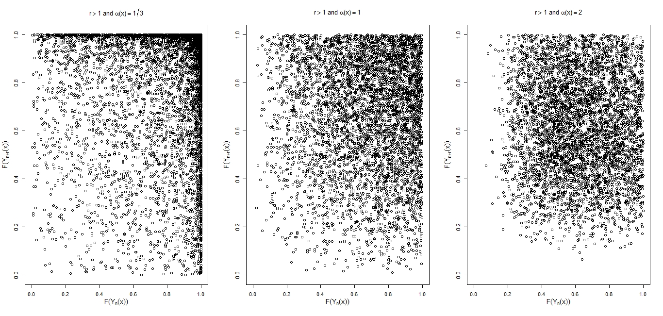
Since the tail dependence coefficient is invariant to increasing transformations one can rather consider λ⁡(F⁡(Yn+r​(x′))|F⁡(Yn​(x))),\lambda(F(Y_{n+r}(x^{\prime}))|F(Y_{n}(x))), n≥1,n\geq 1, r≥0,r\geq 0, x,x′∈ℝ2,x,x^{\prime}\in\mathbb{R}^{2}, where FF is the standard Fréchet distribution function. Observations of pairs (F⁡(Yn​(x)),F⁡(Yn+r​(x′))),(F(Y_{n}(x)),F(Y_{n+r}(x^{\prime}))), n≥1,n\geq 1, r≥0,r\geq 0, x,x′∈ℝ2,x,x^{\prime}\in\mathbb{R}^{2}, are plotted in Figures 1, 2 3 to highlight, respectively, the spatial (r=0r=0 and x≠x′x\neq x^{\prime}), temporal (r>0r>0 and x=x′x=x^{\prime}) and spatial-temporal (r>0r>0 and x≠x′x\neq x^{\prime}) dependence.

Refer to caption
Refer to caption
Refer to caption
Figure 1: Observations of (F⁡(Yn​(x)),F⁡(Yn​(x′)))(F(Y_{n}(x)),F(Y_{n}(x^{\prime}))) n≥1,n\geq 1, x,x′∈ℝ2,x,x^{\prime}\in\mathbb{R}^{2}, x≠x′x\neq x^{\prime} for different values of α⁡(x′)\alpha(x^{\prime}) and α⁡(x)\alpha(x)
Refer to caption
Refer to caption
Figure 2: Observations of (F⁡(Yn​(x)),F⁡(Yn+r​(x)))(F(Y_{n}(x)),F(Y_{n+r}(x))) n≥1,n\geq 1, r≥1,r\geq 1, x∈ℝ2,x\in\mathbb{R}^{2}, for different values α⁡(x)\alpha(x)
Refer to caption
Figure 3: Observations of (F⁡(Yn​(x)),F⁡(Yn+r​(x′)))(F(Y_{n}(x)),F(Y_{n+r}(x^{\prime}))) n≥1,n\geq 1, r>1,r>1, x,x′∈ℝ2,x,x^{\prime}\in\mathbb{R}^{2}, for different values of α⁡(x′)\alpha(x^{\prime}) and α⁡(x)\alpha(x)

For pre-asymptotic dependence, we have temporal

η(x)(Y,r)={max⁡(1/2,α⁡(x)),α(x)<1∧r=11,α(x)≥1∧r=11/2,otherwise.\eta_{(x)}^{(Y,r)}=\left\{\begin{array}[]{ll}\max(1/2,\alpha(x))&,\,\alpha(x)<1\wedge r=1\\ 1&,\,\alpha(x)\geq 1\wedge r=1\\ 1/2&,\,\textrm{otherwise.}\\ \end{array}\right.

space-time η(x′|x)(Y,r)=1/2\eta_{(x^{\prime}|x)}^{(Y,r)}=1/2 and spatial

η(x′|x)(Y)={1,α(x′)≤α(x)≤1α⁡(x)1+α⁡(x),α(x)<1<α(x′)α⁡(x)α⁡(x′),α(x)<1,α(x)<α(x′)<1+α(x)max⁡(12,1α⁡(x′)), 1<α(x)<α(x′)11+α⁡(x′),α(x′)<1<α(x)1α⁡(x),α(x′)<1<α(x)<1+α(x′)max⁡(12,1α⁡(x)), 1<α(x′)<α(x).\eta_{(x^{\prime}|x)}^{(Y)}=\left\{\begin{array}[]{ll}1&,\,\alpha(x^{\prime})\leq\alpha(x)\leq 1\\ \frac{\alpha(x)}{1+\alpha(x)}&,\,\alpha(x)<1<\alpha(x^{\prime})\\ \frac{\alpha(x)}{\alpha(x^{\prime})}&,\,\alpha(x)<1,\alpha(x)<\alpha(x^{\prime})<1+\alpha(x)\\ \max\left(\frac{1}{2},\frac{1}{\alpha(x^{\prime})}\right)&,\,1<\alpha(x)<\alpha(x^{\prime})\\ \frac{1}{1+\alpha(x^{\prime})}&,\,\alpha(x^{\prime})<1<\alpha(x)\\ \frac{1}{\alpha(x)}&,\,\alpha(x^{\prime})<1<\alpha(x)<1+\alpha(x^{\prime})\\ \max\left(\frac{1}{2},\frac{1}{\alpha(x)}\right)&,\,1<\alpha(x^{\prime})<\alpha(x)\,.\end{array}\right.
Example 5.2.

Let us now modify the previous example, so that {X^n​(x),x∈ℝ2}n≥1\{\widehat{X}_{n}(x),\,x\in\mathbb{R}^{2}\}_{n\geq 1} is an i.i.d. sequence of random fields with unit Fréchet margins exhibiting spatial dependence. More precisely, with the dependence between the margins X^n​(x)\widehat{X}_{n}(x) and X^n​(x′)\widehat{X}_{n}(x^{\prime}) given by the Schlather model. Hence, according to Schlather ([8] 2002), X^n​(x)=dX^​(x)\widehat{X}_{n}(x)\stackrel{{\scriptstyle d}}{{=}}\widehat{X}(x) where

X^​(x)=maxi≥1⁡ξi​max​{0,Ui​(x)},x∈ℝ,\widehat{X}(x)=\max_{i\geq 1}\xi_{i}\max\{0,U_{i}(x)\},\quad x\in\mathbb{R},

with {Ui​(x),x∈ℝ}i≥1\{U_{i}(x),x\in\mathbb{R}\}_{i\geq 1} a sequence of independent stationary standard Gaussian processes. For each i≥1,i\geq 1, {Ui​(x),x∈ℝ}i≥1\{U_{i}(x),x\in\mathbb{R}\}_{i\geq 1} has correlation function ρ⁡(h)\rho(h), scaled so that E⁡[max⁡{0,Yi​(x)}]=1E[\max\{0,Y_{i}(x)\}]=1 and {ξi}i≥1\{\xi_{i}\}_{i\geq 1} are the points of a Poisson process on ℝ+\mathbb{R}^{+} with intensity measure ξ−2​d​ξ.\xi^{-2}d\xi. It is a max-stable process (de Haan [2] 1984).

Once again we shall consider {Xn​(x)=23​X^n​(x)∨13​X^n−1​(x),x∈ℝ2}n≥1\{X_{n}(x)=\frac{2}{3}\hat{X}_{n}(x)\vee\frac{1}{3}\hat{X}_{n-1}(x),x\in\mathbb{R}^{2}\}_{n\geq 1} and {Zn​(x)=Zn,x∈ℝ2}n≥1\{Z_{n}(x)=Z_{n},\,x\in\mathbb{R}^{2}\}_{n\geq 1} independent of the previous sequence. For each location x∈ℝ2,x\in\mathbb{R}^{2}, the temporal dependence of {Yn(x)=Xn(x)∨Zn1/α⁡(x)}n≥1\{Y_{n}(x)=X_{n}(x)\vee Z_{n}^{1/\alpha(x)}\}_{n\geq 1} is regulated by the 1-dependence of {Xn​(x)}n≥1,\{X_{n}(x)\}_{n\geq 1}, while the spatial dependence is induced by the common value of ZnZ_{n} in every location and by the correlation ρ⁡(h),\rho(h), where h∈ℝ+h\in\mathbb{R}^{+} is the Euclidean distance between locations xx and x′.x^{\prime}.

For the temporal dependence we find again λ⁡(Yn+r​(x)|Yn​(x)),\lambda(Y_{n+r}(x)|Y_{n}(x)), r≥1,r\geq 1, given in (13), as expected. As to what concerns space-time dependence, for x≠x′,x\neq x^{\prime}, r>1,r>1, n≥1,n\geq 1, λ⁡(Yn+r​(x′)|Yn​(x))=0,\lambda(Y_{n+r}(x^{\prime})|Y_{n}(x))=0, from the 1-dependence of {𝐘n}n≥1.\{{\bf{Y}}_{n}\}_{n\geq 1}. On the other hand, since

P⁡(X^n​(x)≤z,X^n​(x′)≤z′)=exp⁡[−12​(1z+1z′)​(1+1−2​(ρ​(h)+1)​z​z′(z+z′)2)],P(\widehat{X}_{n}(x)\leq z,\widehat{X}_{n}(x^{\prime})\leq z^{\prime})=\exp\left[-\frac{1}{2}\left(\frac{1}{z}+\frac{1}{z^{\prime}}\right)\left(1+\sqrt{1-2(\rho(h)+1)\frac{zz^{\prime}}{(z+z^{\prime})^{2}}}\right)\right],

for x,x′∈ℝ2x,x^{\prime}\in\mathbb{R}^{2} and h=‖x−x′‖,h=\|x-x^{\prime}\|, we find, for x≠x′,x\neq x^{\prime}, n≥1,n\geq 1,

λ⁡(Yn+1​(x′)|Yn​(x))={0,α(x)<112​(1−1−49​(ρ​(h)+1)2),α(x)=11−1−49​(ρ​(h)+1)2,α(x)>1\lambda(Y_{n+1}(x^{\prime})|Y_{n}(x))=\left\{\begin{array}[]{ll}0&,\,\alpha(x)<1\\ \frac{1}{2}\left(\frac{1-\sqrt{1-\frac{4}{9}(\rho(h)+1)}}{2}\right)&,\,\alpha(x)=1\\ \frac{1-\sqrt{1-\frac{4}{9}(\rho(h)+1)}}{2}&,\,\alpha(x)>1\end{array}\right. (14)

and spatial dependence given by

λ⁡(Yn​(x′)|Yn​(x))\displaystyle\lambda(Y_{n}(x^{\prime})|Y_{n}(x)) =\displaystyle= limy→∞[11+y1−α⁡(x)​(1−1−12​(ρ​(h)+1)2)+y−(α⁡(x′)∨α⁡(x))y−1+y−α⁡(x)]\displaystyle\lim_{y\to\infty}\left[\frac{1}{1+y^{1-\alpha(x)}}\left(\frac{1-\sqrt{1-\frac{1}{2}(\rho(h)+1)}}{2}\right)+\frac{y^{-(\alpha(x^{\prime})\vee\alpha(x))}}{y^{-1}+y^{-\alpha(x)}}\right]
=\displaystyle= {1−1−12​(ρ​(h)+1)4+12,α(x)=1∧α(x′)<11−1−12​(ρ​(h)+1)4,α(x)=1∧α(x′)>10,α(x)<1∧α(x′)>α(x)1,α(x)<1∧α(x′)≤α(x)1−1−12​(ρ​(h)+1)2,α(x)>1.\displaystyle\left\{\begin{array}[]{ll}\frac{1-\sqrt{1-\frac{1}{2}(\rho(h)+1)}}{4}+\frac{1}{2}&,\,\alpha(x)=1\ \wedge\ \alpha(x^{\prime})<1\\ \frac{1-\sqrt{1-\frac{1}{2}(\rho(h)+1)}}{4}&,\,\alpha(x)=1\ \wedge\ \alpha(x^{\prime})>1\\ 0&,\,\alpha(x)<1\ \wedge\ \alpha(x^{\prime})>\alpha(x)\\ 1&,\,\alpha(x)<1\ \wedge\ \alpha(x^{\prime})\leq\alpha(x)\\ \frac{1-\sqrt{1-\frac{1}{2}(\rho(h)+1)}}{2}&,\,\alpha(x)>1\end{array}.\right.

When x=x′x=x^{\prime} the result in (14) leads again to (13).

In the forthcoming simulations we shall consider ρ⁡(h)\rho(h) belonging to the powered exponential parametric family, i.e. ρ⁡(h)=exp⁡[−(h/c2)ν],\rho(h)=\exp[-(h/c_{2})^{\nu}], where c2∈]0,+∞[c_{2}\in]0,+\infty[ is the range parameter and ν∈]0,2]\nu\in]0,2] is the smooth parameter, more precisely we shall consider ρ⁡(h)=exp⁡(−h).\rho(h)=\exp(-h).

6 Estimation of model parameters

The pMAX random field defined in (1) sets on parameters α⁡(x)>0\alpha(x)>0 which vary with locations x∈ℝ2.x\in\mathbb{R}^{2}. The estimation of these parameters is essential for practical applications of the model. We shall therefore present a way to estimate α⁡(x)\alpha(x) at a given location x∈ℝ2.x\in\mathbb{R}^{2}.

As previously pointed out, for any location x∈ℝ2x\in\mathbb{R}^{2} the distribution function of Yn​(x),Y_{n}(x), n≥1,n\geq 1, is given by F⁡(z)≡FYn​(x)​(z)=e−z−1−z−α⁡(x),F(z)\equiv F_{Y_{n}(x)}(z)=e^{-z^{-1}-z^{-\alpha(x)}}, for all z>0.z>0. We can then write

α⁡(x)=ln⁡(−ln⁡(F⁡(z))−1z)ln⁡(1z),x∈ℝ2, 0<z≠1.\alpha(x)=\frac{\ln(-\ln(F(z))-\frac{1}{z})}{\ln\left(\frac{1}{z}\right)},\ x\in\mathbb{R}^{2},\ 0<z\neq 1. (16)

We point out that parameter α⁡(x)\alpha(x) “controls” the tail of the distribution F⁡(z),F(z), z>0,z>0, of Yn​(x),Y_{n}(x), n≥1.n\geq 1. Thus, values of α⁡(x)\alpha(x) smaller than one lead to lighter tail distributions than values greater or equal to one.

Expression (16) provides a simple way to estimate the parameter α⁡(x),\alpha(x), x∈ℝ2,x\in\mathbb{R}^{2}, involved in model (1). Therefore, if (Y1,…,Yn)(Y_{1},\ldots,Y_{n}) is a random sample of Yn​(x),Y_{n}(x), n≥1,n\geq 1, for a given x∈ℝ2,x\in\mathbb{R}^{2}, α⁡(x)>0\alpha(x)>0 can be estimated with

α^n​(x)=1n​∑i=1nln⁡(−ln⁡(F^n​(Zi))−1/Zi)ln⁡(1/Zi)\widehat{\alpha}_{n}(x)=\frac{1}{n}\sum_{i=1}^{n}\frac{\ln(-\ln(\widehat{F}_{n}(Z_{i}))-1/Z_{i})}{\ln(1/Z_{i})} (17)

where F^n​(y),\widehat{F}_{n}(y), z∈ℝ,z\in\mathbb{R}, denotes the empirical distribution function, associated to the n−n-sample (Y1,…,Yn),(Y_{1},\ldots,Y_{n}), defined as

F^n(y)=1n∑j=1n1I{Yj≤y},\widehat{F}_{n}(y)=\frac{1}{n}\sum_{j=1}^{n}{1\kern-1.99997pt\rm I}_{\{Y_{j}\leq y\}},

with 1​IA{1\kern-1.99997pt\rm I}_{A} the indicator of an event A.A. The nn values (Z1,…,Zn)(Z_{1},\ldots,Z_{n}) are such that Zi>1Z_{i}>1 and F^n​(Zi)<1,\widehat{F}_{n}(Z_{i})<1, i=1,…,n.i=1,\ldots,n.

In what follows, we explore through simulations the finite sample properties of the proposed estimator (17) for parameter α⁡(x)\alpha(x) at a given location x∈ℝ2.x\in\mathbb{R}^{2}.

Each simulated data set consists of 1000 independent copies of nn realizations of a random sample (Y1,…,Yn)(Y_{1},\ldots,Y_{n}) of (1), with Xn​(x)X_{n}(x) and Zn​(x),Z_{n}(x), at a location x∈ℝ2,x\in\mathbb{R}^{2}, defined as in Examples 5.1 and 5.2, for different values of α⁡(x)>0.\alpha(x)>0. Four different sample sizes are considered for each data set. The sample means μ^​(α^n,i​(x))\widehat{\mu}(\widehat{\alpha}_{n,i}(x)) and the sample standard deviations σ^​(α^n,i​(x))\widehat{\sigma}(\widehat{\alpha}_{n,i}(x)) of the estimates α^n,i​(x),\widehat{\alpha}_{n,i}(x), i=1,…,1000,i=1,\ldots,1000, depending on the sample size n,n, were computed. The bias and the root mean squared errors (R​M​S​E​(α^n,i​(x))RMSE(\widehat{\alpha}_{n,i}(x))) were also determined. The nn values (Z1,…,Zn)(Z_{1},\ldots,Z_{n}) were considered to be an arithmetic sequence of nn numbers from 1.1 to the k​t​hkth percentile of (Y1,…,Yn)(Y_{1},\ldots,Y_{n}), with k=95k=95 and k=75k=75. Tables 1 and 2 summarize the estimation results obtained for the two percentile choices, respectively the 95​t​h95th and the 75​t​h75th percentile.

Table 1: Estimation results for α⁡(x)>0\alpha(x)>0 in model (1) of Example 5.1
95​t​h95th percentile
α⁡(x)\alpha(x) n μ^​(α^n​(x))\widehat{\mu}(\widehat{\alpha}_{n}(x)) B​I​A​S​(α^n​(x))BIAS(\widehat{\alpha}_{n}(x)) σ^​(α^n​(x))\widehat{\sigma}(\widehat{\alpha}_{n}(x)) R​M​S​E​(α^n​(x))RMSE(\widehat{\alpha}_{n}(x))
0.10 n=100n=100 0.1010 0.0010 0.0306 0.0306
n=500n=500 0.0995 -0.0005 0.0071 0.0071
n=1000n=1000 0.1002 0.0002 0.0048 0.0048
n=5000n=5000 0.1000 3.59×10−53.59\times 10^{-5} 0.0020 0.0020
0.50 n=100n=100 0.5027 0.0027 0.0808 0.0808
n=500n=500 0.4981 -0.0019 0.0317 0.0317
n=1000n=1000 0.4994 -0.0006 0.0221 0.0221
n=5000n=5000 0.5000 2.34×10−52.34\times 10^{-5} 0.0095 0.0095
1.00 n=100n=100 1.0212 0.0212 0.2108 0.2118
n=500n=500 1.0079 0.0079 0.0884 0.0887
n=1000n=1000 1.0041 0.0041 0.0604 0.0605
n=5000n=5000 1.0003 0.0003 0.0254 0.0254
1.50 n=100n=100 1.5308 0.0308 0.4014 0.4024
n=500n=500 1.5387 0.0387 0.2243 0.2275
n=1000n=1000 1.5253 0.0253 0.1658 0.1676
n=5000n=5000 1.5045 0.0045 0.0711 0.0712
2.00 n=100n=100 1.9379 -0.0621 0.6186 0.6214
n=500n=500 1.9982 -0.0018 0.3579 0.3577
n=1000n=1000 2.0063 0.0063 0.2971 0.2970
n=5000n=5000 2.0327 0.0327 0.1916 0.1943
75​t​h75th percentile
α⁡(x)\alpha(x) n μ^​(α^n​(x))\widehat{\mu}(\widehat{\alpha}_{n}(x)) B​I​A​S​(α^n​(x))BIAS(\widehat{\alpha}_{n}(x)) σ^​(α^n​(x))\widehat{\sigma}(\widehat{\alpha}_{n}(x)) R​M​S​E​(α^n​(x))RMSE(\widehat{\alpha}_{n}(x))
0.10 n=100n=100 0.1008 0.00081 0.0367 0.0367
n=500n=500 0.1000 4.42×10−54.42\times 10^{-5} 0.0084 0.0084
n=1000n=1000 0.1000 4.85×10−54.85\times 10^{-5} 0.0056 0.0056
n=5000n=5000 0.1000 2.39×10−52.39\times 10^{-5} 0.0024 0.0024
0.50 n=100n=100 0.5060 0.0060 0.1319 0.1320
n=500n=500 0.5040 0.0040 0.0527 0.0528
n=1000n=1000 0.5012 0.0012 0.0372 0.0372
n=5000n=5000 0.5008 0.0008 0.0161 0.0161
1.00 n=100n=100 1.0387 0.0387 0.2927 0.2951
n=500n=500 1.0051 0.0051 0.1173 0.1174
n=1000n=1000 1.0003 0.0003 0.0806 0.0805
n=5000n=5000 1.0001 9.61×10−59.61\times 10^{-5} 0.0349 0.0349
1.50 n=100n=100 1.5452 0.0452 0.4753 0.4772
n=500n=500 1.5124 0.0124 0.1866 0.1869
n=1000n=1000 1.5029 0.0029 0.1289 0.1289
n=5000n=5000 1.4994 -0.0006 0.0566 0.0566
2.00 n=100n=100 2.1143 0.1143 0.6962 0.7052
n=500n=500 2.0322 0.0322 0.2734 0.2752
n=1000n=1000 2.0222 0.0222 0.1914 0.1926
n=5000n=5000 2.0005 0.0005 0.0843 0.0843
Table 2: Estimation results for α⁡(x)>0\alpha(x)>0 in model (1) of Example 5.2
95​t​h95th percentile
α⁡(x)\alpha(x) n μ^​(α^n​(x))\widehat{\mu}(\widehat{\alpha}_{n}(x)) B​I​A​S​(α^n​(x))BIAS(\widehat{\alpha}_{n}(x)) σ^​(α^n​(x))\widehat{\sigma}(\widehat{\alpha}_{n}(x)) R​M​S​E​(α^n​(x))RMSE(\widehat{\alpha}_{n}(x))
0.10 n=100n=100 0.0994 -0.0006 0.0311 0.0311
n=500n=500 0.1001 0.0001 0.0069 0.0069
n=1000n=1000 0.1001 0.0001 0.0047 0.0047
n=5000n=5000 0.0999 -6.28×10⁻⁵\times 10^{-5} 0.0021 0.0021
0.50 n=100n=100 0.5027 0.0027 0.0822 0.0822
n=500n=500 0.4993 -0.0007 0.03199 0.03120
n=1000n=1000 0.4999 -8.34 0.0208 0.0208
n=5000n=5000 0.5000 2.39×10⁻⁵\times 10^{-5} 0.0096 0.0096
1.00 n=100n=100 1.0345 0.0345 0.2294 0.2319
n=500n=500 1.0057 0.0057 0.0851 0.0853
n=1000n=1000 1.0013 0.0013 0.0576 0.0576
n=5000n=5000 1.0005 0.0005 0.0264 0.0264
1.50 n=100n=100 1.5286 0.0286 0.4206 0.4214
n=500n=500 1.5336 0.0336 0.2315 0.2338
n=1000n=1000 1.5316 0.0316 0.1739 0.1766
n=5000n=5000 1.5048 0.0048 0.0715 0.0716
2.00 n=100n=100 1.9551 -0.0449 0.6755 0.6767
n=500n=500 2.0069 0.0069 0.3582 0.3580
n=1000n=1000 2.0242 0.0242 0.2998 0.3006
n=5000n=5000 2.0378 0.0378 0.1904 0.1941
75​t​h75th percentile
α⁡(x)\alpha(x) n μ^​(α^n​(x))\widehat{\mu}(\widehat{\alpha}_{n}(x)) B​I​A​S​(α^n​(x))BIAS(\widehat{\alpha}_{n}(x)) σ^​(α^n​(x))\widehat{\sigma}(\widehat{\alpha}_{n}(x)) R​M​S​E​(α^n​(x))RMSE(\widehat{\alpha}_{n}(x))
0.10 n=100n=100 0.1000 4.33×10⁻⁵\times 10^{-5} 0.0369 0.0368
n=500n=500 0.1002 0.0002 0.0086 0.0086
n=1000n=1000 0.1003 0.0003 0.0056 0.0057
n=5000n=5000 0.1001 8.43×10⁻⁵\times 10^{-5} 0.0022 0.0022
0.50 n=100n=100 0.5078 0.0078 0.1366 0.1367
n=500n=500 0.5013 0.0013 0.0530 0.0530
n=1000n=1000 0.5011 0.0011 0.0365 0.0365
n=5000n=5000 0.5006 0.0006 0.0160 0.0160
1.00 n=100n=100 1.0403 0.0403 0.2974 0.3000
n=500n=500 1.0011 0.0011 0.1159 0.1159
n=1000n=1000 1.0032 0.0032 0.0820 0.0820
n=5000n=5000 1.0014 0.0014 0.0371 0.0371
1.50 n=100n=100 1.5511 0.0511 0.4414 0.4442
n=500n=500 1.5099 0.0099 0.1764 0.1766
n=1000n=1000 1.5037 0.0037 0.1270 0.1269
n=5000n=5000 1.5029 0.0029 0.0571 0.0572
2.00 n=100n=100 2.0734 0.0734 0.6760 0.6797
n=500n=500 2.0269 0.0269 0.2774 0.2785
n=1000n=1000 2.0119 0.0119 0.1861 0.1864
n=5000n=5000 2.0068 0.0068 0.0843 0.0845

The results of Tables 1 and 2 show that the proposed estimator for α⁡(x)\alpha(x) has an overall good performance. Due to the tail weight of F⁡(z)F(z) the estimator has a better behavior for α⁡(x)<1\alpha(x)<1 (light tail) when the empirical distribution function is evaluated to higher percentiles of the data, whereas for α⁡(x)≥1\alpha(x)\geq 1 (heavy tail) better results are obtained when the empirical distribution function is evaluated to lower percentiles of the data.

7 Discussion

The pMAX model presented in this work is another contribution to the modeling of heavy tail random fields. The α⁡(x)\alpha(x) parameter allows for an encompassing extreme dependency structure, including asymptotic and pre-asymptotic dependence. If α⁡(x)\alpha(x) is less than or equal to 1, its value affects the measures of dependence, λ⁡(Yn​(x′)|Yn​(x))\lambda(Y_{n}(x^{\prime})|Y_{n}(x)) and η(x′|x)(Y),\eta_{(x^{\prime}|x)}^{(Y)}, that were considered here. In this case, α⁡(x)\alpha(x) also corresponds to the tail index of the marginal Yn​(x)Y_{n}(x), so it can be estimated as such.

References

  • [1] Buishand, T., De Haan, L., Zhou, C. On Spatial Extremes: With Application to a Rainfall Problem. Ann. App. Stat., 2(2), 624-642 (2008)
  • [2] de Haan, L. A spectral representation for max-stable processes. Ann. Probab., 12, 1194-1204 (1984)
  • [3] Ferreira, H., Ferreira, M. Extremal behavior of pMAX processes. Stat. Prob. Letters, 93C, 46-57 (2014)
  • [4] Heffernan, J.E., Tawn, J.A., Zhang, Z. Asymptotically (in)dependent multivariate maxima of moving maxima processes. Extremes, 10, 57-82 (2007)
  • [5] Hristopulos, D.T. Random Fields for Spatial Data Modeling. A Primer for Scientists and Engineers. Springer, Dordrecht (2020)
  • [6] Joe H. Multivariate Models and Dependence Concepts. Monographs on Statistics and Applied Probability 73. Chapman and Hall, London (1997)
  • [7] Ledford, A., Tawn, J.A. Statistics for near independence in multivariate extreme values. Biometrika, 83, 169-187 (1996)
  • [8] Schlather, M. Models for stationary max-stable random fields. Extremes, 5(1), 33-44 (2002)
  • [9] Sibuya, M. Bivariate extreme statistics. Ann. Inst. Statist. Math., 11, 195-210 (1960)