Decay of semigroup for an infinite interacting particle system on continuum configuration spaces

Chenlin Gu Chenlin GuDMA, Ecole normale supérieure, PSL University, Paris, France

Abstract.

We show the heat kernel type variance decay $t^{-\frac{d}{2}}$ , up to a logarithmic correction, for the semigroup of an infinite particle system on ${\mathbb{R}^{d}}$ , where every particle evolves following a divergence-form operator with diffusivity coefficient that depends on the local configuration of particles. The proof relies on the strategy from [30], and generalizes the localization estimate to the continuum configuration space introduced by S. Albeverio, Y.G. Kondratiev and M. Röckner.

MSC 2010: 82C22, 35B65, 60K35.

Keywords: interacting particle system, heat kernel estimate, configuration space.

1. Introduction

In this work, we study an interacting diffusive particle system in ${\mathbb{R}^{d}}$ and the heat kernel type estimate for its semigroup. Let us give an informal introduction to the model and main result at first. We denote by $\mathcal{M}_{\delta}({\mathbb{R}^{d}})$ the set of point measures of type $\mu=\sum_{i=1}^{\infty}\delta_{x_{i}}$ on ${\mathbb{R}^{d}}$ , which we call configurations of particles, by $\mathcal{F}_{U}$ the $\sigma$ -algebra generated by $\mu(V)$ tested with all the Borel set $V\subseteq U$ , and use the shorthand $\mathcal{F}:=\mathcal{F}_{{\mathbb{R}^{d}}}$ . Let $\mathbb{P}_{\rho}$ be the Poisson point process of density $\rho\in(0,\infty)$ as the law for the configuration $\mu$ , with $\mathbb{E}_{\rho},\mathbb{V}\!\mathrm{ar}_{\rho}$ the associated expectation and variance. We have $\mathbf{a}_{\circ}:\mathcal{M}_{\delta}({\mathbb{R}^{d}})\to\mathbb{R}^{d\times d}_{sym}$ an $\mathcal{F}_{B_{1}}$ -measurable symmetric matrix, i.e. it only depends on the configuration in the unit ball $B_{1}$ , and $|\xi|^{2}\leqslant\xi\cdot\mathbf{a}_{\circ}\xi\leqslant\Lambda|\xi|^{2}$ for any $\xi\in{\mathbb{R}^{d}}$ . Then let $\mathbf{a}(\mu,x):=\mathbf{a}_{\circ}(\tau_{-x}\mu)$ be the diffusive coefficient with local interaction at $x$ , where $\tau_{-x}$ represents the transport operation by the direction $-x$ . Denoting by ${\mu_{t}:=\sum_{i=1}^{\infty}\delta_{x_{i,t}}}$ the configuration at time $t\geqslant 0$ , our model can be informally described as an infinite-dimensional system with local interaction such that every particle $x_{i,t}$ evolves as a diffusion associated to the divergence-form operator $-\nabla\cdot\mathbf{a}(\mu_{t},x_{i,t})\nabla$ . More precisely, it is a Markov process $\left(\Omega,(\mathscr{F}_{t})_{t\geqslant 0},\mathbb{P}_{\rho}\right)$ defined by the Dirichlet form

(1.1)

\displaystyle\mathcal{E}^{\mathbf{a}}(f,f):=\mathbb{E}_{\rho}\left[\int_{{\mathbb{R}^{d}}}\nabla f(\mu,x)\cdot\mathbf{a}(\mu,x)\nabla f(\mu,x)\,{\mathrm{d}}\mu(x)\right],

where the directional derivative ${\mathbf{e}_{k}\cdot\nabla f(\mu,x):=\lim_{h\to 0}\frac{1}{h}(f(\mu-\delta_{x}+\delta_{x+h\mathbf{e}_{k}})-f(\mu))}$ along the canonical direction $\{\mathbf{e}_{k}\}_{1\leqslant k\leqslant d}$ is defined for a family of suitable functions and $x\in\supp(\mu)$ .

One may expect that the diffusion follows the heat kernel estimate established by the pioneering work of John Nash [38], as every single particle is a diffusion of divergence type. This is the object of our main theorem. Let $u:\mathcal{M}_{\delta}({\mathbb{R}^{d}})\to\mathbb{R}$ be an $\mathcal{F}$ -measurable function, depending only on the configuration in the cube $Q_{l_{u}}:=\left[-\frac{l_{u}}{2},\frac{l_{u}}{2}\right]^{d}$ , and smooth with respect to the transport of every particle ( i.e. $u$ belongs to the function space $C^{\infty}_{c}(\mathcal{M}_{\delta}({\mathbb{R}^{d}}))$ defined in Section 2.1.2), and let $u_{t}:=\mathbb{E}_{\rho}[u(\mu_{t})|\mathscr{F}_{0}]$ . Denoting $L^{\infty}:=L^{\infty}(\mathcal{M}_{\delta}({\mathbb{R}^{d}}),\mathcal{F},\mathbb{P}_{\rho})$ , we have the following estimate.

Theorem 1.1 (Decay of variance).

There exists two finite positive constants ${\gamma:=\gamma(\rho,d,\Lambda)}$ , ${C:=C(\rho,d,\Lambda)}$ such that for any $u\in C^{\infty}_{c}(\mathcal{M}_{\delta}({\mathbb{R}^{d}}))$ supported in $Q_{l_{u}}$ , then we have

(1.2)

\displaystyle\mathbb{V}\!\mathrm{ar}_{\rho}[u_{t}]\leqslant C(1+|\log t|)^{\gamma}\left(\frac{1+l_{u}}{\sqrt{t}}\right)^{d}\|u\|^{2}_{L^{\infty}}.

Interacting particle systems remain an active research topic, and it is hard to list all the references. We refer to the excellent monographs [32, 33, 34, 42] for a panorama of the field. In recent years, many works in probability and stochastic processes illustrate the diffusion universality in various models: a well-understood model is the random conductance model, see [14] for a survey, and especially the heat kernel bound and invariance principle is established for the percolation clusters in [13, 37, 41, 36, 11, 12, 40]; from the view point of stochastic homogenization, the quantitative results are also proved in a series of work [9, 6, 10, 7, 26, 27, 23, 24, 25], and the monograph [8], and these techiques also apply on the percolation clusters setting, as shown in [5, 19, 28, 20]; for the system of hard-spheres, Bodineau, Gallagher and Saint-Raymond prove that Brownian motion is the Boltzmann-Grad limit of a tagged particle in [16, 15, 17]. All these works make us believe that the model in this work should also have diffusive behavior in large scale or long time.

Notice that our model is of non-gradient type, and our result is established in the continuum configuration space rather than a function space on ${\mathbb{R}^{d}}$ . In previous works, the construction of similar diffusion processes is studied by Albeverio, Kondratiev and Röckner using Dirichlet forms in [1, 2, 3, 4]; see also the survey [39]. To the best of our knowledge, we do not find Theorem 1.1 in the literature. While in the lattice side, let us remark one important work [30] by Janvresse, Landim, Quastel and Yau, where the decay of variance is proved in the ${\mathbb{Z}^{d}}$ zero range model, which is of gradient type. Since our research is inspired by [30] and also uses some of their techniques, we point out our contributions in the following.

Firstly, we give an explicit bound with respect to the size of the support of the local function $u$ , that is uniform over $t$ ; the bound $\left(\frac{l_{u}}{\sqrt{t}}\right)^{d}$ captures the correct typical scale. For comparison, [30, Theorem 1.1] states the result

(1.3)

\displaystyle\mathbb{V}\!\mathrm{ar}_{\rho}[u_{t}]=\frac{[\widetilde{u}^{\prime}(\rho)]^{2}\chi(\rho)}{[8\pi\phi^{\prime}(\rho)t]^{\frac{d}{2}}}+o\left(t^{-\frac{d}{2}}\right),

which should be considered as the asymptotic behavior in long time, and the term $o\left(t^{-\frac{d}{2}}\right)$ is of type $(l_{u})^{5d}t^{-\left(\frac{d}{2}+\varepsilon\right)}$ if one tracks carefully the dependence of $l_{u}$ in the steps of the proof of [30, Theorem 1.1]. To get the typical scale $\left(\frac{l_{u}}{\sqrt{t}}\right)^{d}$ , we do some combinatorial improvement in the intermediate coarse-graining argument in eq. 3.14; see also Figure 1 for illustration. On the other hand, we also wonder if we could establish a similar result as eq. 1.3 to identify the diffusive constant in the long time behavior. This an interesting question and one perspective in future research, but a major difficulty here is to characterize the effective diffusion constant, because the zero range model satisfies the gradient condition while our model does not. We believe that it is related to the bulk diffusion coefficient and the equilibrium density fluctuation in the lattice nongradient model as indicated in [42, eq.(2.14), Proposition 2.1].

Secondly, we extend a localization estimate to the continuum configuration space: under the same context of Theorem 1.1, and recalling that $\mathcal{F}_{Q_{K}}$ represents the information of $\mu$ in the cube ${Q_{K}=\left[-\frac{K}{2},\frac{K}{2}\right]^{d}}$ , we define ${\mathcal{A}}_{K}u_{t}:=\mathbb{E}_{\rho}[u_{t}|\mathcal{F}_{Q_{K}}]$ , and show that for every ${t\geqslant\max\left\{(l_{u})^{2},16\Lambda^{2}\right\}}$ and $K\geqslant\sqrt{t}$

(1.4)

\mathbb{E}_{\rho}\left[(u_{t}-{\mathcal{A}}_{K}u_{t})^{2}\right]\leqslant C(\Lambda)\exp\left(-\frac{K}{\sqrt{t}}\right)\mathbb{E}_{\rho}\left[u^{2}\right].

This is a key estimate appearing in [30, Proposition 3.1], and is also natural as $\sqrt{t}$ is the typical scale of diffusion, thus when $K\gg\sqrt{t}$ one get very good approximation in eq. 1.4. Its generalization in the continuum configuration space is non-trivial, since in the proof of [30, Proposition 3.1], one tests the Dirichlet form with ${\mathcal{A}}_{K}u_{t}$ , but in our model it is not in the domain of Dirichlet form $\mathcal{D}(\mathcal{E}^{\mathbf{a}})$ and one cannot put ${\mathcal{A}}_{K}u_{t}$ directly in the Dirichlet form eq. 1.1. This is one essential difference between our model and a lattice model. To solve it, we have to apply some regularization steps which we present in Theorem 4.1.

Finally, we remark kindly a minor error in the proof in [30] and fix it when revisiting the paper. This will be presented in Section 3.1 and Remark 3.3.

The rest of this article is organized as follows. In Section 2, we define all the notations and the rigorous construction of our model. Section 3 is the main part of the proof of Theorem 1.1, where Section 3.1 gives its outline and we fix the minor error in [30] mentioned above. The proof of some technical estimates used in Section 3 are put in the last two sections, where Section 4 proves the localization estimate eq. 1.4 in continuum configuration space, and Section 5 serves as a toolbox of other estimates including spectral inequality, perturbation estimate and calculation of the entropy.

2. Preliminaries

2.1. Notations

In this part, we introduce the notations used in this paper. We write ${\mathbb{R}^{d}}$ for the $d$ -dimensional Euclidean space, $B_{r}(x)$ for the ball of radius $r$ centered at $x$ , and $Q_{s}(x):=x+\left[-\frac{s}{2},\frac{s}{2}\right]^{d}$ as the cube of edge length $s$ centered at $x$ . We also denote by $B_{r}$ and $Q_{s}$ respectively short for $B_{r}(0)$ and $Q_{s}(0)$ . The lattice set is defined by $\mathcal{Z}_{s}:={\mathbb{Z}^{d}}\cap Q_{s}$ .

2.1.1. Continuum configuration space

For any metric space $(E,d)$ , we denote by $\mathcal{M}(E)$ the set of Radon measures on $E$ . For every Borel set $U\subseteq E$ , we denote by $\mathcal{F}_{U}$ the smallest $\sigma$ -algebra such that for every Borel subset $V\subseteq U$ , the mapping ${\mu\in\mathcal{M}(E)\mapsto\mu(V)}$ is measurable. For a $\mathcal{F}_{U}$ -measurable function $f:\mathcal{M}(E)\to\mathbb{R}$ , we say that $f$ supported in $U$ i.e. $\supp(f)\subseteq U$ . In the case $\mu\in\mathcal{M}(E)$ is of finite total mass, we write

(2.1)

\strokedint f\,{\mathrm{d}}\mu:=\frac{\int f\,{\mathrm{d}}\mu}{\int{\mathrm{d}}\mu}.

We also define the collection of point measure $\mathcal{M}_{\delta}(E)\subseteq\mathcal{M}(E)$

\displaystyle\mathcal{M}_{\delta}(E):=\left\{\mu\in\mathcal{M}(E):\mu=\sum_{i\in I}\delta_{x_{i}}\text{ for some }I\text{ finite or countable},\text{ and }x_{i}\in E\text{ for any }i\in I\right\},

which serves as the continuum configuration space where each Dirac measure stands the position of a particle. In this work we will mainly focus on the Euclidean space ${\mathbb{R}^{d}}$ and its associated point measure space $\mathcal{M}_{\delta}({\mathbb{R}^{d}})$ , and use the shorthand notation $\mathcal{F}:=\mathcal{F}_{{\mathbb{R}^{d}}}$ .

We define two operations for elements in $\mathcal{M}_{\delta}({\mathbb{R}^{d}})$ : restriction and transport.

•

For every $\mu\in\mathcal{M}_{\delta}({\mathbb{R}^{d}})$ and Borel set $U\subseteq{\mathbb{R}^{d}}$ , we define the restriction operation $\mu\mathbin{\vrule height=6.02773pt,depth=0.0pt,width=0.55974pt\vrule height=0.55974pt,depth=0.0pt,width=4.30554pt}U$ , such that for every Borel set $V\subseteq{\mathbb{R}^{d}}$ , $(\mu\mathbin{\vrule height=6.02773pt,depth=0.0pt,width=0.55974pt\vrule height=0.55974pt,depth=0.0pt,width=4.30554pt}U)(V)=\mu(U\cap V)$ . Then for a function $f:\mathcal{M}_{\delta}({\mathbb{R}^{d}})\to\mathbb{R}$ which is $\mathcal{F}_{U}$ -measurable, we have $f(\mu)=f(\mu\mathbin{\vrule height=6.02773pt,depth=0.0pt,width=0.55974pt\vrule height=0.55974pt,depth=0.0pt,width=4.30554pt}U)$ .
•

The transport on the set is defined as

$\displaystyle\forall h\in{\mathbb{R}^{d}},U\subseteq{\mathbb{R}^{d}},\tau_{h}U:=\{y+h:y\in U\}.$

Then for every $\mu\in\mathcal{M}_{\delta}({\mathbb{R}^{d}})$ and $h\in{\mathbb{R}^{d}}$ , we define the transport operation $\tau_{h}\mu$ such that for every Borel set $U$ , we have

(2.2) $\displaystyle\tau_{h}\mu(U):=\mu(\tau_{-h}U).$

For $f$ an $\mathcal{F}_{V}$ -measurable function, we also define the transport operation $\tau_{h}f$ as a pullback that

(2.3) $\displaystyle\tau_{h}f(\mu):=f(\tau_{-h}\mu),$

which is an $\mathcal{F}_{\tau_{h}V}$ -measurable function.

Notice that the restriction operation can be defined similarly in $\mathcal{M}(E)$ for a metric space, but the transport operation requires that $E$ is at least a vector space.

We fix $\rho>0$ once and for all, and define $\mathbb{P}_{\rho}$ a probability measure on $(\mathcal{M}_{\delta}({\mathbb{R}^{d}}),\mathcal{F})$ , to be the Poisson measure on ${\mathbb{R}^{d}}$ with density $\rho$ (see [31]). We denote by $\mathbb{E}_{\rho}$ the expectation, $\mathbb{V}\!\mathrm{ar}_{\rho}$ the variance associated with the law $\mathbb{P}_{\rho}$ , and by $\mu$ the canonical $\mathcal{M}_{\delta}({\mathbb{R}^{d}})$ -valued random variable on the probability space $(\mathcal{M}_{\delta}({\mathbb{R}^{d}}),\mathcal{F},\mathbb{P}_{\rho})$ . In the case $U\subseteq{\mathbb{R}^{d}}$ a bounded Borel set and $f$ a $\mathcal{F}_{U}$ -measurable function, we can rewrite the expectation $\mathbb{E}_{\rho}[f]$ in an explicit expression

(2.4)

\mathbb{E}_{\rho}\left[f\right]=\sum_{N=0}^{+\infty}e^{-\rho|U|}\frac{(\rho|U|)^{N}}{N!}\strokedint_{U^{N}}f\left(\sum_{i=1}^{N}\delta_{x_{i}}\right)\,{\mathrm{d}}x_{1}\cdots{\mathrm{d}}x_{N}.

For instance, for every bounded Borel set $U\subseteq{\mathbb{R}^{d}}$ and bounded measurable function $g:U\to\mathbb{R}$ , we can write

\mathbb{E}_{\rho}\left[\int_{U}g(x)\,{\mathrm{d}}\mu(x)\right]=\rho\int_{U}g(x)\,{\mathrm{d}}x.

Notice that the measure $\mu$ is a Poisson point process under $\mathbb{P}_{\rho}$ . In particular, the measures $\mu\mathbin{\vrule height=6.02773pt,depth=0.0pt,width=0.55974pt\vrule height=0.55974pt,depth=0.0pt,width=4.30554pt}U$ and $\mu\mathbin{\vrule height=6.02773pt,depth=0.0pt,width=0.55974pt\vrule height=0.55974pt,depth=0.0pt,width=4.30554pt}({\mathbb{R}^{d}}\setminus U)$ are independent, and the conditional expectation $\mathbb{E}_{\rho}\left[\cdot|\mathcal{F}_{({\mathbb{R}^{d}}\setminus U)}\right]$ can thus be described equivalently as an averaging over the law of $\mu\mathbin{\vrule height=6.02773pt,depth=0.0pt,width=0.55974pt\vrule height=0.55974pt,depth=0.0pt,width=4.30554pt}U$ .

For any $1\leqslant p<\infty$ , we denote by $L^{p}(\mathcal{M}_{\delta}(U))$ the set of $\mathcal{F}_{U}$ -measurable functions $f:\mathcal{M}_{\delta}(U)\to\mathbb{R}$ such that the norm

\|f\|_{L^{p}(\mathcal{M}_{\delta}(U))}:=\left(\mathbb{E}_{\rho}\left[|f|^{p}\right]\right)^{\frac{1}{p}}

is finite and $L^{p}$ short for $L^{p}(\mathcal{M}_{\delta}({\mathbb{R}^{d}}))$ . We denote by $L^{\infty}(\mathcal{M}_{\delta}(U))$ the norm defined by essential upper bound under $\mathbb{P}_{\rho}$ .

2.1.2. Derivative and $C_{c}^{\infty}(\mathcal{M}_{\delta}(U))$

We define the directional derivative for a $\mathcal{F}_{U}$ -measurable function $f:\mathcal{M}_{\delta}(U)\to\mathbb{R}$ . Let $\{\mathbf{e}_{k}\}_{1\leqslant k\leqslant n}$ be $d$ canonical directions, for $x\in\supp(\mu)$ , we define

\displaystyle\partial_{k}f(\mu,x):=\lim_{h\to 0}\frac{1}{h}(f(\mu-\delta_{x}+\delta_{x+h\mathbf{e}_{k}})-f(\mu)),

if the limit exists, and the gradient as a vector

\displaystyle{\nabla f(\mu,x):=(\partial_{1}f(\mu,x),\partial_{2}f(\mu,x),\cdots\partial_{d}f(\mu,x))}.

One can define the function with higher derivative iteratively, but here we use a more natural way: for every Borel set $U\subseteq{\mathbb{R}^{d}}$ and $N\in\mathbb{N}$ , let $\mathcal{M}_{\delta}(U,N)\subseteq\mathcal{M}_{\delta}(E)$ be defined as

\displaystyle\mathcal{M}_{\delta}(U,N):=\left\{\mu\in\mathcal{M}_{\delta}({\mathbb{R}^{d}}):\mu=\sum_{i=1}^{N}x_{i},x_{i}\in U\text{ for every }1\leqslant i\leqslant N\right\}.

Then a function $f:\mathcal{M}_{\delta}(U,N)\to\mathbb{R}$ can be identified with a function $\widetilde{f}:U^{N}\to\mathbb{R}$ by setting

(2.5)

\widetilde{f}(x)=\widetilde{f}(x_{1},\ldots,x_{N}):=f\left(\sum_{i=1}^{N}\delta_{x_{i}}\right).

The function $\widetilde{f}$ is invariant under permutations of its $N$ coordinates. Conversely, any function satisfying this symmetry can be identified with a function from $\mathcal{M}_{\delta}(U,N)$ to $\mathbb{R}$ . We denote by $C^{\infty}(\mathcal{M}_{\delta}(U,N))$ the set of functions $f:\mathcal{M}_{\delta}(U,N)\to\mathbb{R}$ such that $\widetilde{f}$ is infinitely differentiable. For every $f\in C^{\infty}(\mathcal{M}_{\delta}(U,N))$ and $x_{1},\ldots,x_{N}\in U$ , the gradient at $x_{1}$ coincides with the its canonical sense for the coordinate $x_{1}$ .

(2.6)

\nabla f\left(\sum_{i=1}^{N}\delta_{x_{i}},x_{1}\right)=\nabla_{x_{1}}\widetilde{f}(x_{1},\ldots,x_{N}).

We denote by $C^{\infty}_{c}(\mathcal{M}_{\delta}(U))$ the set of functions $f:\mathcal{M}_{\delta}(U)\to\mathbb{R}$ that satisfy:

(1)

there exists a compact Borel set $V\subseteq U$ such that $f$ is $\mathcal{F}_{V}$ -measurable;

(2)

for every $N\in\mathbb{N}$ ,

\text{the mapping }\left\{\begin{array}[]{rcl}\mathcal{M}_{\delta}(U,N)&\to&\mathbb{R}\\ \mu&\mapsto&f(\mu)\end{array}\right.\mbox{belongs to $C^{\infty}(\mathcal{M}_{\delta}(U,N))$.}

(3)

the function is bounded.

A more heuristic description for $f\in C^{\infty}_{c}(\mathcal{M}_{\delta}(U))$ is a function uniformly bounded, depending only on the information in a compact subset $V\subseteq U$ , and when we do projection $f(\mu)=f(\mu\mathbin{\vrule height=6.02773pt,depth=0.0pt,width=0.55974pt\vrule height=0.55974pt,depth=0.0pt,width=4.30554pt}V)$ it can be identified as a function $C^{\infty}$ with finite coordinate, and also smooth when the number of particles in $V$ changes.

2.1.3. Sobolev space on $\mathcal{M}_{\delta}(U)$

We define the $H^{1}(\mathcal{M}_{\delta}(U))$ norm by

\|f\|_{H^{1}(\mathcal{M}_{\delta}(U))}:=\left(\|f\|_{L^{2}(\mathcal{M}_{\delta}(U))}^{2}+\mathbb{E}_{\rho}\left[\int_{U}|\nabla f|^{2}\,{\mathrm{d}}\mu\right]\right)^{\frac{1}{2}},

and let $H^{1}_{0}(\mathcal{M}_{\delta}(U))$ denote the completion with respect to this norm of the space

\left\{f\in C^{\infty}_{c}(\mathcal{M}_{\delta}(U))\ :\ \|f\|_{H^{1}(\mathcal{M}_{\delta}(U))}<\infty\right\}.

2.2. Construction of model

2.2.1. Diffusion coefficient

In this part, we define the coefficient field of the diffusion. We give ourselves a symmetric matrix valued function $\mathbf{a}_{\circ}:\mathcal{M}_{\delta}({\mathbb{R}^{d}})\to\mathbb{R}^{d\times d}_{sym}$ which satisfies the following properties:

•

uniform ellipticity: there exists $\Lambda\in[1,+\infty)$ such that for every $\mu\in\mathcal{M}_{\delta}({\mathbb{R}^{d}})$ and every $\xi\in{\mathbb{R}^{d}}$ ,

(2.7) $|\xi|^{2}\leqslant\xi\cdot\mathbf{a}_{\circ}(\mu)\xi\leqslant\Lambda|\xi|^{2}\,;$
•

locality: for every $\mu\in\mathcal{M}_{\delta}({\mathbb{R}^{d}})$ , $\mathbf{a}_{\circ}(\mu)=\mathbf{a}_{\circ}\left(\mu\mathbin{\vrule height=6.02773pt,depth=0.0pt,width=0.55974pt\vrule height=0.55974pt,depth=0.0pt,width=4.30554pt}B_{1}\right)$ .

We extend $\mathbf{a}_{\circ}$ by stationarity using the transport operation defined in eq. 2.3: for every $\mu\in\mathcal{M}_{\delta}({\mathbb{R}^{d}})$ and $x\in{\mathbb{R}^{d}}$ ,

\mathbf{a}(\mu,x):=\tau_{x}\mathbf{a}_{\circ}(\mu)=\mathbf{a}_{\circ}(\tau_{-x}\mu).

A typical example of a coefficient field $\mathbf{a}$ of interest is ${\mathbf{a}_{\circ}(\mu):=(1+\mathbf{1}_{\{\mu(B_{1})=1\}}})\mathbf{Id}$ whose extension is given by $\mathbf{a}(\mu,x):=(1+\mathbf{1}_{\{\mu(B_{1}(x))=1\}})\mathbf{Id}$ . In words, for $x\in\supp(\mu)$ , the quantity $\mathbf{a}(\mu,x)$ is equal to $2$ whenever there is no other point than $x$ in the unit ball around $x$ , and is equal to $1$ otherwise.

2.2.2. Markov process defined by Dirichlet form

In this part, we construct our infinite particle system on $\mathcal{M}_{\delta}({\mathbb{R}^{d}})$ by Dirichlet form (see [21, 35] for the notations). We define at first the non-negative bilinear symmetric form

\displaystyle\mathcal{E}^{\mathbf{a}}(f,g):=\mathbb{E}_{\rho}\left[\int_{{\mathbb{R}^{d}}}\nabla f(\mu,x)\cdot\mathbf{a}(\mu,x)\nabla g(\mu,x)\,{\mathrm{d}}\mu(x)\right],

on its domain $\mathcal{D}(\mathcal{E}^{\mathbf{a}})$ that

\displaystyle\mathcal{D}(\mathcal{E}^{\mathbf{a}}):=H^{1}_{0}(\mathcal{M}_{\delta}({\mathbb{R}^{d}})).

We also use $\mathcal{E}^{\mathbf{a}}(f):=\mathcal{E}^{\mathbf{a}}(f,f)$ for short. It is clear that $\mathcal{E}^{\mathbf{a}}$ is closed and Markovian thus it is a Dirichlet form, so it defines the correspondence between the Dirichlet form and the generator $\mathcal{L}$ that

\displaystyle\mathcal{E}^{\mathbf{a}}(f,g)=\mathbb{E}_{\rho}\left[f(-\mathcal{L})g\right],\qquad\mathcal{D}(\mathcal{E}^{\mathbf{a}})=\mathcal{D}(-\mathcal{L}).

and a $L^{2}(\mathcal{M}_{\delta}({\mathbb{R}^{d}}))$ strongly continuous Markov semigroup $(P_{t})_{t\geqslant 0}$ . We denote by $(\mathscr{F}_{t})_{t\geqslant 0}$ its filtration and $(\mu_{t})_{t\geqslant 0}$ the associated $\mathcal{M}_{\delta}({\mathbb{R}^{d}})$ -valued Markov process which stands the configuration of the particles, then for any $u\in L^{2}(\mathcal{M}_{\delta}({\mathbb{R}^{d}}))$ ,

\displaystyle u_{t}(\mu):=P_{t}u(\mu)=\mathbb{E}_{\rho}[u(\mu_{t})|\mathscr{F}_{0}],

is an element in $\mathcal{D}(\mathcal{E}^{\mathbf{a}})$ and is characterized by the parabolic equation on $\mathcal{M}_{\delta}({\mathbb{R}^{d}})$ that for any $v\in\mathcal{D}(\mathcal{E}^{\mathbf{a}})$

(2.8)

\displaystyle\mathbb{E}_{\rho}[u_{t}v]-\mathbb{E}_{\rho}[uv]=-\int_{0}^{t}\mathcal{E}^{\mathbf{a}}(u_{s},v)\,{\mathrm{d}}s.

Finally, we remark that the average is conserved for $u_{t}$ as we test eq. 2.8 by constant $1$ that

(2.9)

\displaystyle\mathbb{E}_{\rho}[u_{t}]-\mathbb{E}_{\rho}[u]=-\int_{0}^{t}\mathbb{E}_{\rho}\left[\int_{{\mathbb{R}^{d}}}\nabla 1\cdot\mathbf{a}(\mu,x)\nabla u_{s}(\mu,x)\,{\mathrm{d}}\mu\right]\,{\mathrm{d}}s=0.

In this work, we focus more on the quantitative property of $P_{t}$ ; see [39] for more details about the trajectory property of similar type of process.

2.3. A solvable case

We propose a solvable model to illustrate that the behavior of this process is close to the diffusion and the rate of decay is the best one that we can expect.

In the following, we suppose that $\mathbf{a}=\frac{1}{2}$ which means that in fact every particle evolves as a Brownian motion i.e. $\mu=\sum_{i=1}^{\infty}\delta_{x_{i}}$ , $\mu_{t}=\sum_{i=1}^{\infty}\delta_{B^{(i)}_{t}}$ that $\left(B^{(i)}_{t}\right)_{t\geqslant 0}$ is a Brownian motion issued from $x_{i}$ and $\left(B^{(i)}_{\cdot}\right)_{i\in\mathbb{N}}$ is independent.

Example 2.1.

Let $u(\mu):=\int_{{\mathbb{R}^{d}}}f\,{\mathrm{d}}\mu$ with $f\in C^{\infty}_{c}({\mathbb{R}^{d}})$ . In this case, we have

\displaystyle u_{t}(\mu)=P_{t}u(\mu)

\displaystyle=\mathbb{E}_{\rho}\left[u(\mu_{t})|\mathscr{F}_{0}\right]=\mathbb{E}_{\rho}\left[\left.\sum_{i\in\mathbb{N}}f\left(B^{(i)}_{t}\right)\right|\mathscr{F}_{0}\right]=\int_{{\mathbb{R}^{d}}}f_{t}(x)\,{\mathrm{d}}\mu(x),

where $f_{t}\in C^{\infty}({\mathbb{R}^{d}})$ is the solution of the Cauchy problem of the standard heat equation: ${\Phi_{t}(x)=\frac{1}{(2\pi t)^{\frac{d}{2}}}\exp\left(-\frac{|x|^{2}}{2t}\right)}$ and $f_{t}(x)=\Phi_{t}\star f(x)$ . Then we use the formula of variance for Poisson process

	$\displaystyle\mathbb{V}\!\mathrm{ar}_{\rho}\left[u\right]$	$\displaystyle=\rho\int_{{\mathbb{R}^{d}}}f^{2}(x)\,{\mathrm{d}}x=\rho\\|f\\|^{2}_{L^{2}\left({\mathbb{R}^{d}}\right)},$
	$\displaystyle\mathbb{V}\!\mathrm{ar}_{\rho}\left[u_{t}\right]$	$\displaystyle=\rho\int_{{\mathbb{R}^{d}}}f_{t}^{2}(x)\,{\mathrm{d}}x=\rho\\|f_{t}\\|^{2}_{L^{2}\left({\mathbb{R}^{d}}\right)}.$

By the heat kernel estimate for the standard heat equation, we known that ${\|f_{t}\|^{2}_{L^{2}({\mathbb{R}^{d}})}\simeq C(d)t^{-\frac{d}{2}}\|f\|^{2}_{L^{1}({\mathbb{R}^{d}})}}$ , thus the scale $t^{-\frac{d}{2}}$ is the best one that we can obtain. Moreover, if we take $f=\mathbf{1}_{\left\{Q_{r}\right\}}$ , and ${t=r^{2(1-\varepsilon)}}$ for a small $\varepsilon>0$ , then we see that the typical scale of diffusion is a ball of size $r^{1-\varepsilon}$ . So for every $x\in Q_{r\left(1-r^{-\frac{\varepsilon}{2}}\right)}$ , the value $f_{t}(x)\simeq 1-e^{-r^{\frac{\varepsilon}{2}}}$ and we have

\displaystyle\mathbb{V}\!\mathrm{ar}_{\rho}\left[u_{t}\right]=\rho\int_{{\mathbb{R}^{d}}}f_{t}^{2}(x)\,{\mathrm{d}}x\geqslant\rho r^{d}(1-r^{-\frac{\varepsilon}{2}})=(1-r^{-\frac{\varepsilon}{2}})\mathbb{V}\!\mathrm{ar}_{\rho}\left[u\right].

It illustrates that before the scale $t=r^{2}$ , the decay is very slow so in the Theorem 1.1 the factor $\left(\frac{l_{u}}{\sqrt{t}}\right)^{d}$ is reasonable.

3. Strategy of proof

In this part, we state the strategy of the proof of Theorem 1.1. We will give a short outline in Section 3.1, which can be see as an “approximation-variance decomposition”, and then focus on the term approximation in Section 3.2. Several technical estimates will be used in this procedure and their proofs will be postponed in Section 4 and Section 5.

3.1. Outline

As mentionned, this work is inspired from [30], and we revisit the strategy here. We pick a centered $u\in C^{\infty}_{c}(\mathcal{M}_{\delta}({\mathbb{R}^{d}}))$ supported in $Q_{l_{u}}$ such that $\mathbb{E}_{\rho}[u]=0$ and this implies $\mathbb{E}_{\rho}[u_{t}]=0$ from eq. 2.9. Then we set a multi-scale $\{t_{n}\}_{n\geqslant 0},t_{n+1}=Rt_{n}$ , where $R>1$ is a scale factor to be fixed later. It suffices to prove that eq. 1.2 for every $t_{n}$ , then for $t\in[t_{n},t_{n+1}]$ , one can use the decay of $L^{2}$ that

\displaystyle\mathbb{E}_{\rho}[(u_{t})^{2}]\leqslant\mathbb{E}_{\rho}[(u_{t_{n}})^{2}]\leqslant C(1+\log(t_{n}))^{\gamma}\left(\frac{1+l_{u}}{\sqrt{t_{n}}}\right)^{d}\|u\|^{2}_{L^{\infty}}\leqslant CR^{\frac{d}{2}}(1+\log t)^{\gamma}\left(\frac{1+l_{u}}{\sqrt{t}}\right)^{d}\|u\|^{2}_{L^{\infty}},

then by resetting the constant $C$ one concludes the main theorem. Another ingredient of the proof is an “approximation-variance type decomposition”:

(3.1)

\begin{split}u_{t}&=v_{t}+w_{t},\\ v_{t}&:=u_{t}-\frac{1}{|\mathcal{Z}_{K}|}\sum_{y\in\mathcal{Z}_{K}}\tau_{y}u_{t},\\ w_{t}&:=\frac{1}{|\mathcal{Z}_{K}|}\sum_{y\in\mathcal{Z}_{K}}\tau_{y}u_{t},\end{split}

where we recall $\mathcal{Z}_{K}=Q_{K}\cap{\mathbb{Z}^{d}}$ is the lattice set of scale $K$ . The philosophy of this decomposition is that in long time, the information in a local scale $K$ is mixed, thus $w_{t}$ as a spatial average is a good approximation of $u_{t}$ and $v_{t}$ is the error term. Thus, the following control Proposition 3.1 and Proposition 5.2 of the two terms $w_{t}$ and $v_{t}$ proves the main theorem Theorem 1.1.

Proposition 3.1.

There exists a finite positive number $C:=C(d)$ such that for any ${u\in C^{\infty}_{c}(\mathcal{M}_{\delta}({\mathbb{R}^{d}}))}$ with mean zero, supported in $Q_{l_{u}}$ and for any $K\geqslant l_{u}$ , we have

(3.2)

\displaystyle\mathbb{V}\!\mathrm{ar}_{\rho}\left[\left(\frac{1}{|\mathcal{Z}_{K}|}\sum_{y\in\mathcal{Z}_{K}}\tau_{y}u_{t}\right)^{2}\right]\leqslant C(d)\left(\frac{l_{u}}{K}\right)^{d}\mathbb{E}_{\rho}[u^{2}].

Proof.

Then we can estimate the variance simply by $L^{2}$ decay that

\mathbb{E}_{\rho}[(w_{t})^{2}]=\mathbb{E}_{\rho}\left[\left(P_{t}\left(\frac{1}{|\mathcal{Z}_{K}|}\sum_{y\in\mathcal{Z}_{K}}\tau_{y}u\right)\right)^{2}\right]\leqslant\mathbb{E}_{\rho}\left[\left(\frac{1}{|\mathcal{Z}_{K}|}\sum_{y\in\mathcal{Z}_{K}}\tau_{y}u\right)^{2}\right]=\frac{1}{|\mathcal{Z}_{K}|^{2}}\sum_{x,y\in\mathcal{Z}_{K}}\mathbb{E}_{\rho}\left[(\tau_{x-y}u)u\right].

We know that for $|x-y|\geqslant l_{u}$ , then the term $\tau_{x-y}u$ and $u$ is independent so $\mathbb{E}_{\rho}\left[(\tau_{x-y}u)u\right]$ = 0. This concludes eq. 3.2. ∎

Proposition 3.2.

There exists two finite positive numbers $C:=C(d,\rho),\gamma:=\gamma(d,\rho)$ such that for any ${u\in C^{\infty}_{c}(\mathcal{M}_{\delta}({\mathbb{R}^{d}}))}$ supported in $Q_{l_{u}}$ , $K\geqslant l_{u}$ and $v_{t}$ defined in eq. 3.1, for ${t_{n}\geqslant\max\left\{l_{u}^{2},16\Lambda^{2}\right\}},t_{n+1}=Rt_{n}$ with $R>1$ we have

(3.3)

\displaystyle(t_{n+1})^{\frac{d+2}{2}}\mathbb{E}_{\rho}[(v_{t_{n+1}})^{2}]-(t_{n})^{\frac{d+2}{2}}\mathbb{E}_{\rho}[(v_{t_{n}})^{2}]\leqslant C(\log(t_{n+1}))^{\gamma}K^{2}(l_{u})^{d}\|u\|^{2}_{L^{\infty}}+\mathbb{E}_{\rho}[u^{2}].

Proof of Theorem 1.1 from Proposition 3.2 and Proposition 3.1.

For the case $t\leqslant(l_{u})^{2}$ or ${t\leqslant 16\Lambda^{2}}$ , the right hand side of eq. 1.2 is larger than $\mathbb{E}_{\rho}[u^{2}]$ and we can use the $L^{2}$ decay to prove the theorem. Thus without loss of generality, we set ${t_{0}:=\max\left\{l_{u}^{2},16\Lambda^{2}\right\}}$ and put eq. 3.3 into eq. 1.2 by setting $K:=\sqrt{t_{n+1}}$ that

(3.4)

\begin{split}&\mathbb{E}_{\rho}[(u_{t_{n+1}})^{2}]\\ \leqslant&2\mathbb{E}_{\rho}[(v_{t_{n+1}})^{2}]+2\mathbb{E}_{\rho}[(w_{t_{n+1}})^{2}]\\ \leqslant&2\left(\frac{t_{n}}{t_{n+1}}\right)^{\frac{d+2}{2}}\mathbb{E}_{\rho}[(v_{t_{n}})^{2}]+2(t_{n+1})^{-\frac{d+2}{2}}\left(C(\log(t_{n+1}))^{\gamma}t_{n+1}(l_{u})^{d}\|u\|^{2}_{L^{\infty}}+\mathbb{E}_{\rho}[u^{2}]\right)\\ &\qquad\qquad+2\mathbb{E}_{\rho}[(w_{t_{n+1}})^{2}]\\ \leqslant&4\left(\frac{t_{n}}{t_{n+1}}\right)^{\frac{d+2}{2}}\mathbb{E}_{\rho}[(u_{t_{n}})^{2}]+2(t_{n+1})^{-\frac{d+2}{2}}\left(C(\log(t_{n+1}))^{\gamma}t_{n+1}(l_{u})^{d}\|u\|^{2}_{L^{\infty}}+\mathbb{E}_{\rho}[u^{2}]\right)\\ &\qquad+4\left(\frac{t_{n}}{t_{n+1}}\right)^{\frac{d+2}{2}}\mathbb{E}_{\rho}[(w_{t_{n}})^{2}]+2\mathbb{E}_{\rho}[(w_{t_{n+1}})^{2}].\end{split}

We set $U_{n}=(t_{n})^{\frac{d}{2}}\mathbb{E}_{\rho}[(u_{t_{n}})^{2}]$ and put eq. 3.2 into the equation above, we have

\displaystyle U_{n+1}\leqslant\theta U_{n}+C_{2}\left((\log(t_{n+1}))^{\gamma}(l_{u})^{d}\|u\|^{2}_{L^{\infty}}+(t_{n+1})^{-1}\mathbb{E}_{\rho}[u^{2}]\right)+C_{3}(l_{u})^{d}\mathbb{E}_{\rho}[u^{2}],

where $\theta=4R^{-1}$ . By choosing $R$ large such that $\theta\in(0,1)$ , we do a iteration for the equation above to obtain that

	$\displaystyle U_{n+1}$	$\displaystyle\leqslant\sum_{k=1}^{n}\left(C_{2}\left((\log(t_{n+1}))^{\gamma}(l_{u})^{d}\\|u\\|^{2}_{L^{\infty}}+\mathbb{E}_{\rho}[u^{2}]\right)+C_{3}(l_{u})^{d}\mathbb{E}_{\rho}[u^{2}]\right)\theta^{n-k}+U_{0}\theta^{n+1}$
		$\displaystyle\leqslant\frac{1}{1-\theta}\left(C_{2}\left((\log(t_{n+1}))^{\gamma}(l_{u})^{d}\\|u\\|^{2}_{L^{\infty}}+\mathbb{E}_{\rho}[u^{2}]\right)+C_{3}(l_{u})^{d}\mathbb{E}_{\rho}[u^{2}]\right)+(l_{u})^{d}\mathbb{E}_{\rho}[u^{2}]$
	$\displaystyle\Longrightarrow$	$\displaystyle\mathbb{E}_{\rho}[(u_{t_{n+1}})^{2}]\leqslant C_{4}(\log(t_{n+1}))^{\gamma}\left(\frac{l_{u}}{\sqrt{t_{n+1}}}\right)^{d}\\|u\\|^{2}_{L^{\infty}}.$

∎

Remark 3.3.

We remark that there is a small error in the similar argument in [30, Proof of Proposition 2.2]: the authors apply eq. 3.3 from $t_{0}$ to $t_{n}$ , and they neglect the change of scale in $K$ at the endpoints $\{t_{n}\}_{n\geqslant 0}$ . However, it does not harm the whole proof and we fix it here: we add one more step of decomposition in eq. 3.4, and put the iteration directly in $u_{t}$ instead of $v_{t}$ , which avoids the problem of the changes of $K$ .

3.2. Error for the approximation

In this part, we prove Proposition 3.2. The proof can be divided into 6 steps.

Proof of Proposition 3.2.

. Step 1: Setting up. To shorten the equation, we define

(3.5)

\displaystyle\Delta_{n}:=(t_{n+1})^{\frac{d+2}{2}}\mathbb{E}_{\rho}[(v_{t_{n+1}})^{2}]-(t_{n})^{\frac{d+2}{2}}\mathbb{E}_{\rho}[(v_{t_{n}})^{2}],

and it is the goal of the whole subsection. In the step setting up, we do derivative for the flow $t^{\frac{d+2}{2}}\mathbb{E}_{\rho}[(v_{t})^{2}]$ that

(3.6)

\displaystyle\Delta_{n}=\int_{t_{n}}^{t_{n+1}}\left(\frac{d+2}{2}\right)t^{\frac{d}{2}}\mathbb{E}_{\rho}[(v_{t})^{2}]-2t^{\frac{d+2}{2}}\mathbb{E}_{\rho}[v_{t}(-\mathcal{L}v_{t})]\,{\mathrm{d}}t.

Step 2: Localization. We set ${\mathcal{A}}_{L}v_{t}:=\mathbb{E}\left[v_{t}|\mathcal{F}_{Q_{L}}\right]$ and use it to approximate $v_{t}$ in $L^{2}$ . Since it is a diffusion process, one can guess naturally a scale larger than $\sqrt{t}$ will have enough information for this approximation. In Theorem 4.1 we prove an estimate

\displaystyle\mathbb{E}_{\rho}\left[(v_{t}-{\mathcal{A}}_{L}v_{t})^{2}\right]\leqslant C(\Lambda)\exp\left(-\frac{L}{\sqrt{t}}\right)\mathbb{E}_{\rho}\left[(v_{0})^{2}\right],

and we choose $L=\lfloor\gamma\log(t_{n+1})\rfloor\sqrt{t_{n+1}},\gamma>\frac{d+4}{2}$ here, and put it back to eq. 3.6 to obtain

(3.7)

\begin{split}\Delta_{n}\leqslant&\int_{t_{n}}^{t_{n+1}}(d+2)t^{\frac{d}{2}}\mathbb{E}_{\rho}\left[\left({\mathcal{A}}_{L}v_{t}\right)^{2}\right]+(d+2)t^{\frac{d}{2}-\gamma}\mathbb{E}_{\rho}\left[(v_{0})^{2}\right]-2t^{\frac{d+2}{2}}\mathbb{E}_{\rho}[v_{t}(-\mathcal{L}v_{t})]\,{\mathrm{d}}t\\ \leqslant&\mathbb{E}_{\rho}[(u_{0})^{2}]+\int_{t_{n}}^{t_{n+1}}(d+2)t^{\frac{d}{2}}\mathbb{E}_{\rho}\left[\left({\mathcal{A}}_{L}v_{t}\right)^{2}\right]-2t^{\frac{d+2}{2}}\mathbb{E}_{\rho}[v_{t}(-\mathcal{L}v_{t})]\,{\mathrm{d}}t.\end{split}

Step 3: Approximation by density. We apply a second approximation: we choose another scale $l>0$ , whose value will be fixed but $L/l\in\mathbb{N}$ and $l\simeq\sqrt{t_{n+1}}$ . We denote by $q=(L/l)^{d}$ and $\mathbf{M}_{L,l}=(\mathbf{M}_{1},\mathbf{M}_{2}\cdots\mathbf{M}_{q})$ a random vector, where $\mathbf{M}_{i}$ is the number of the particle in $i$ -th cube of scale $l$ . Then we define an operator

\displaystyle\mathcal{B}_{L,l}v_{t}:=\mathbb{E}_{\rho}\left[v_{t}|\mathbf{M}_{L,l}\right].

The main idea here is that the random vector $\mathbf{M}_{L,l}$ captures the information of convergence, once we know the density in every cube of scale $l\simeq\sqrt{t_{n+1}}$ converges to $\rho$ . In Proposition 5.1 we will prove a spectral inequality that

\displaystyle\mathbb{E}_{\rho}\left[({\mathcal{A}}_{L}v_{t}-\mathcal{B}_{L,l}v_{t})^{2}\right]\leqslant R_{0}l^{2}\mathbb{E}_{\rho}\left[v_{t}(-\mathcal{L}v_{t})\right].

We put this estimate into eq. 3.7

	$\displaystyle\Delta_{n}\leqslant$	$\displaystyle\mathbb{E}_{\rho}[(u_{0})^{2}]+\int_{t_{n}}^{t_{n+1}}2(d+2)t^{\frac{d}{2}}\mathbb{E}_{\rho}\left[\left(\mathcal{B}_{L,l}v_{t}\right)^{2}\right]+2t^{\frac{d}{2}}((d+2)R_{0}l^{2}-t)\mathbb{E}_{\rho}[v_{t}(-\mathcal{L}v_{t})]\,{\mathrm{d}}t$
	$\displaystyle\leqslant$	$\displaystyle\mathbb{E}_{\rho}[(u_{0})^{2}]+\int_{t_{n}}^{t_{n+1}}2(d+2)t^{\frac{d}{2}}\mathbb{E}_{\rho}\left[\left(\mathcal{B}_{L,l}v_{t}\right)^{2}\right]\,{\mathrm{d}}t,$

where we obtain the last line by choosing a scale $l=c\sqrt{t_{n+1}}$ such that $(d+2)R_{0}l^{2}\leqslant t_{n}$ and $L/l\in\mathbb{N}$ .

It remains to estimate how small $\mathbb{E}_{\rho}\left[\left(\mathcal{B}_{L,l}v_{t}\right)^{2}\right]$ is. The typical case is that the density is close to $\rho$ in every cube of scale $l$ in $Q_{L}$ . Let us define $M=(M_{1},M_{2},\cdots M_{q})$ , and we have

\displaystyle\mathcal{B}_{L,l}v_{t}(M)=\mathbb{E}_{\rho}\left[v_{t}|\mathbf{M}_{L,l}=M\right].

Then we call $\mathcal{C}_{L,l,\rho,\delta}$ the $\delta$ -good configuration that

(3.8)

\displaystyle\mathcal{C}_{L,l,\rho,\delta}:=\left\{M\in\mathbb{N}^{q}\left|\forall 1\leqslant i\leqslant q,\left|\frac{M_{i}}{\rho|Q_{l}|}-1\right|\leqslant\delta\right.\right\}.

We can use standard Chernoff bound and union bound to prove the upper bound of $\mathbb{P}_{\rho}\left[\mathbf{M}_{L,l}\notin\mathcal{C}_{L,l,\rho,\delta}\right]$ : for any $\lambda>0$ , we have

	$\displaystyle\mathbb{P}_{\rho}\left[\exists\leqslant i\leqslant q,\frac{\mathbf{M}_{i}}{\rho\|Q_{l}\|}\geqslant 1+\delta\right]$	$\displaystyle\leqslant\left(\frac{L}{l}\right)^{d}\exp(-\lambda(1+\delta))\mathbb{E}_{\rho}\left[\exp\left(\frac{\lambda\mu(Q_{l})}{\rho\|Q_{l}\|}\right)\right]$
		$\displaystyle=\left(\frac{L}{l}\right)^{d}\exp\left(-\lambda(1+\delta)+\rho\|Q_{l}\|\left(e^{\frac{\lambda}{\rho\|Q_{l}\|}}-1\right)\right)$
		$\displaystyle\leqslant\left(\frac{L}{l}\right)^{d}\exp\left(-\lambda\delta+\frac{\lambda^{2}}{\rho\|Q_{l}\|}\right).$

In the second line we use the exact Laplace transform for $\mu(Q_{l})$ as we know ${\mu(Q_{l})\stackrel{{\scriptstyle\text{law}}}{{\sim}}\text{Poisson}(\rho|Q_{l}|)}$ . Then we do optimization by choosing $\lambda=\frac{\delta\rho|Q_{l}|}{2}$ . The other side is similar and we conclude

(3.9)

\displaystyle\mathbb{P}_{\rho}\left[\mathbf{M}_{L,l}\notin\mathcal{C}_{L,l,\rho,\delta}\right]\leqslant\left(\gamma\log(t_{n+1})\right)^{d}\exp\left(-\frac{\rho|Q_{l}|\delta^{2}}{4}\right).

For the case $M\notin\mathcal{C}_{L,l,\rho,\delta}$ , we can bound $\mathcal{B}_{L,l}v_{t}(M)$ naively by $|\mathcal{B}_{L,l}v_{t}(M)|\leqslant C\|u_{0}\|_{L^{\infty}}$ , thus we have

\displaystyle\mathbb{E}_{\rho}\left[\left(\mathcal{B}_{L,l}v_{t}\right)^{2}\right]\leqslant\sum_{M\in\mathcal{C}_{L,l,\rho,\delta}}\mathbb{P}_{\rho}[\mathbf{M}_{L,l}=M](\mathcal{B}_{L,l}v_{t}(M))^{2}+\left(\gamma\log(t_{n+1})\right)^{d}\exp\left(-\frac{\rho|Q_{l}|\delta^{2}}{4}\right)\|u_{0}\|^{2}_{L^{\infty}}

and we finish this step by

(3.10)

\begin{split}\Delta_{n}\leqslant&\mathbb{E}_{\rho}[(u_{0})^{2}]+(t_{n+1})^{\frac{d+2}{2}}\left(\gamma\log(t_{n+1})\right)^{d}\exp\left(-\frac{\rho|Q_{l}|\delta^{2}}{4}\right)\|u_{0}\|^{2}_{L^{\infty}}\\ &\qquad+\sum_{M\in\mathcal{C}_{L,l,\rho,\delta}}\mathbb{P}_{\rho}[\mathbf{M}_{L,l}=M]\int_{t_{n}}^{t_{n+1}}2(d+2)t^{\frac{d}{2}}(\mathcal{B}_{L,l}v_{t}(M))^{2}\,{\mathrm{d}}t.\end{split}

We remark that the parameter $\delta>0$ will be fixed at the end of the proof.

Step 4: Perturbation estimate. It remains to estimate the term $(\mathcal{B}_{L,l}v_{t}(M))^{2}$ for the the $\delta$ -good configuration. Now we put the expression of $v_{t}$ in and obtain

\displaystyle(\mathcal{B}_{L,l}v_{t}(M))^{2}

\displaystyle=\left(\frac{1}{|\mathcal{Z}_{K}|}\sum_{y\in\mathcal{Z}_{K}}(\mathcal{B}_{L,l}(u_{t}-\tau_{y}u_{t}))(M)\right)^{2},

and our aim is to control

(3.11)

\begin{split}\int_{t_{n}}^{t_{n+1}}2(d+2)t^{\frac{d}{2}}\left(\frac{1}{|\mathcal{Z}_{K}|}\sum_{y\in\mathcal{Z}_{K}}(\mathcal{B}_{L,l}(u_{t}-\tau_{y}u_{t}))(M)\right)^{2}\,{\mathrm{d}}t.\end{split}

To treat eq. 3.11, we calculate the Radon-Nikodym derivative that

(3.12)

\displaystyle g_{M}:=\frac{{\mathrm{d}}\mathbb{P}_{\rho}[\cdot|\mathbf{M}_{L,l}=M]}{{\mathrm{d}}\mathbb{P}_{\rho}}=\frac{1}{\mathbb{P}_{\rho}[\mathbf{M}_{L,l}=M]]}\mathbf{1}_{\left\{\mathbf{M}_{L,l}=M]\right\}}.

Then we use the reversibility of the semigroup $P_{t}$ and denote by $g_{M,t}:=P_{t}g_{M}$

\displaystyle\mathcal{B}_{L,l}(u_{t}-\tau_{y}u_{t})(M)=\mathbb{E}_{\rho}[g_{M}(u_{t}-\tau_{y}u_{t})]=\mathbb{E}_{\rho}\left[g_{M,t}(u-\tau_{y}u)\right].

Then we would like to apply the a perturbation estimate Proposition 5.2 to control it: let $l_{k}:=l_{u}+2k$ then for any $|y|\leqslant k$ , we have

\displaystyle\mathbb{E}_{\rho}[g_{M}(u_{t}-\tau_{y}u_{t})]\leqslant C(d)(l_{k}\|u\|_{L^{\infty}})^{2}\mathcal{E}_{Q_{l_{k}}}(\sqrt{g_{M}}),

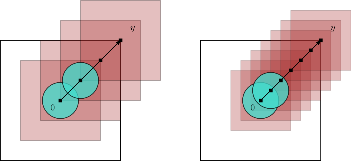
where $\mathcal{E}_{Q_{l_{k}}}(\sqrt{g_{M}})$ is a localized Dirichlet form defined in eq. 5.4. A heuristic analysis of order is $\mathcal{E}_{Q_{l_{k}}}(\sqrt{g_{M}})\simeq O\left((l_{k})^{d}\right)$ since it is a Dirichlet form on $Q_{l_{k}}$ . If we choose $k=K$ here to cover all the term, the bound will be of order $O(K^{d})$ , which is big when $K\simeq\sqrt{t}\geqslant l_{u}$ . Therefore, we apply a coarse-graining argument: let $\overline{[0,y]}_{k}:=\{z_{i}\}_{0\leqslant i\leqslant n(y)}$ be a lattice path that of scale $k$ , ${z_{0}=0},{z_{n(y)}=y},{\{z_{i}\}_{1\leqslant i<n(y)}\in(k\mathbb{Z})^{d}}$ so the length of path is the shortest one. (See Figure 1 for illustration.) Then we have

\displaystyle(u-\tau_{y}u)=\sum_{i=0}^{n(y)-1}(\tau_{z_{i}}u-\tau_{z_{i+1}}u)=\sum_{i=0}^{n(y)-1}\tau_{z_{i}}(u-\tau_{h_{z_{i}}}u),

where $h_{z_{i}}=z_{i+1}-z_{i}$ the vector connecting the two and $|h_{z_{i}}|\leqslant k$ . This expression with the transport invariant law of Poisson point process, Cauchy-Schwartz inequality implies

(3.13)

\begin{split}\left(\mathcal{B}_{L,l}(u_{t}-\tau_{y}u_{t})(M)\right)^{2}&=\left(\sum_{z\in\overline{[0,y]}_{k}}\mathbb{E}_{\rho}\left[g_{M,t}\tau_{z}(u-\tau_{h_{z}}u)\right]\right)^{2}\\ &=\left(\sum_{z\in\overline{[0,y]}_{k}}\mathbb{E}_{\rho}\left[\left(\tau_{-z}g_{M,t}\right)(u-\tau_{h_{z}}u)\right]\right)^{2}\\ &\leqslant C(d)n(y)\sum_{z\in\overline{[0,y]}_{k}}\left(\mathbb{E}_{\rho}\left[\left(\tau_{-z}g_{M,t}\right)(u-\tau_{h_{z}}u)\right]\right)^{2}.\end{split}

This term appears a perturbation estimate, which will be proved in Proposition 5.2 that

	$\displaystyle\left(\mathbb{E}_{\rho}\left[\left(\tau_{-z}g_{M,t}\right)(u-\tau_{h_{z}}u)\right]\right)^{2}$	$\displaystyle\leqslant C(d)(l_{k}\\|u\\|_{L^{\infty}})^{2}\mathcal{E}_{Q_{l_{k}}}\left(\sqrt{\tau_{-z}g_{M,t}}\right)$
		$\displaystyle=C(d)(l_{k}\\|u\\|_{L^{\infty}})^{2}\mathcal{E}_{\tau_{z}Q_{l_{k}}}\left(\sqrt{g_{M,t}}\right),$

where in the last step we use the transport invariant property of Poisson point process. Now we turn to the choice of the scale $k$ . By the heuristic analysis that every $\mathcal{E}_{Q_{l_{k}}}$ contributes order $O((l_{k})^{d})$ and taking in account $n(y)\leqslant K/k$ we have in eq. 3.13

\displaystyle\left(\mathcal{B}_{L,l}(u_{t}-\tau_{y}u_{t})(M)\right)^{2}\simeq O\left(\left(\frac{K}{k}\right)^{2}(l_{k})^{d+2}\right)\simeq O\left(\left(\frac{K}{k}\right)^{2}(l_{u}+2k)^{d+2}\right).

From this we see that a good scale should be $k=l_{u}$ so the term above is of order $O(K^{2}(l_{u})^{d})$ . We put these estimate back to eq. 3.11

(3.14)

\text{\lx@cref{creftype\lx@tilde refnum}{eq:PerTwo}}\leqslant\|u\|^{2}_{L^{\infty}}\int_{t_{n}}^{t_{n+1}}2(d+2)t^{\frac{d}{2}}Kl_{u}\left(\frac{1}{|\mathcal{Z}_{K}|}\sum_{y\in\mathcal{Z}_{K}}\sum_{z\in\overline{[0,y]}_{l_{u}}}\mathcal{E}_{\tau_{z}Q_{3l_{u}}}\left(\sqrt{g_{M,t}}\right)\right)\,{\mathrm{d}}t.

Refer to caption — Figure 1. The illustration of the coarse-graining argument, where we take a lattice path of scale $k$ to connect $0$ and $y$ . The ball in blue is the support of $u$ and the box in red is $Q_{l_{k}}$ . For the one on the left, the scale is $k=l_{u}$ ; the one on the right the scale is finer and we see that the coarse-graining is too dense.

Step 5: Covering argument. In this step, we calculate the right hand side of eq. 3.14, where we notice one essential problem: there are totally about $K^{d+1}/l_{u}$ terms of Dirichlet form $\mathcal{E}_{\tau_{z}Q_{3l_{u}}}\left(\sqrt{g_{M,t}}\right)$ in the sum $\sum_{y\in\mathcal{Z}_{K}}\sum_{z\in\overline{[0,y]}_{l_{u}}}\mathcal{E}_{\tau_{z}Q_{l_{u}}}\left(\sqrt{g_{M,t}}\right)$ , but the one with $z$ close to $0$ are counted of order $K^{d}$ times, while the one with $z$ near $\partial\mathcal{Z}_{K}$ are counted only constant times. To solve this problem, we have to reaverage the sum: by the transport invariant property of Poisson point process, at the beginning of the Step 1, we can write

\displaystyle\Delta_{n}=\frac{1}{|\mathcal{Z}_{l}|}\sum_{x\in\mathcal{Z}_{l}}\left((t_{n+1})^{\frac{d+2}{2}}\mathbb{E}_{\rho}[(\tau_{x}v_{t_{n+1}})^{2}]-(t_{n})^{\frac{d+2}{2}}\mathbb{E}_{\rho}[(\tau_{x}v_{t_{n}})^{2}]\right).

Then all estimates works in Step 1, Step 2 and Step 3 work by replacing ${v_{t}\mapsto\tau_{x}v_{t}}$ and ${u_{t}\mapsto\tau_{x}u_{t}}$ . In the Step 4, this operation will change our object term eq. 3.11

\displaystyle\text{\lx@cref{creftype\lx@tilde refnum}{eq:PerTwo}-avg}=\int_{t_{n}}^{t_{n+1}}2(d+2)t^{\frac{d}{2}}\left(\frac{1}{|\mathcal{Z}_{l}|}\sum_{w\in\mathcal{Z}_{l}}\frac{1}{|\mathcal{Z}_{K}|}\sum_{y\in\mathcal{Z}_{K}}(\mathcal{B}_{L,l}\tau_{w}(u_{t}-\tau_{y}u_{t})(M))^{2}\right)\,{\mathrm{d}}t,

and the perturbation argument Proposition 5.2 reduces the problem as

(3.15)

\text{\lx@cref{creftype\lx@tilde refnum}{eq:PerTwo}-avg}\leqslant\|u\|^{2}_{L^{\infty}}\int_{t_{n}}^{t_{n+1}}2(d+2)t^{\frac{d}{2}}Kl_{u}\\ \qquad\qquad\times\left(\frac{1}{|\mathcal{Z}_{l}|}\sum_{w\in\mathcal{Z}_{l}}\frac{1}{|\mathcal{Z}_{K}|}\sum_{y\in\mathcal{Z}_{K}}\sum_{z\in\overline{[0,y]}_{l_{u}}}\mathcal{E}_{\tau_{w+z}Q_{3l_{u}}}\left(\sqrt{g_{M,t}}\right)\right)\,{\mathrm{d}}t.\\

Now we can apply the Fubini’s lemma

		$\displaystyle\frac{1}{\|\mathcal{Z}_{l}\|}\sum_{w\in\mathcal{Z}_{l}}\frac{1}{\|\mathcal{Z}_{K}\|}\sum_{y\in\mathcal{Z}_{K}}\sum_{z\in\overline{[0,y]}_{l_{u}}}\mathcal{E}_{\tau_{w+z}Q_{3l_{u}}}\left(\sqrt{g_{M,t}}\right)$
	$\displaystyle=$	$\displaystyle\frac{1}{\|\mathcal{Z}_{l}\|}\frac{1}{\|\mathcal{Z}_{K}\|}\mathbb{E}_{\rho}\left[\int_{{\mathbb{R}^{d}}}\left(\sum_{w\in\mathcal{Z}_{l}}\sum_{y\in\mathcal{Z}_{K}}\sum_{z\in\overline{[0,y]}_{l_{u}}}\mathbf{1}_{\left\{x\in\tau_{w+z}Q_{3l_{u}}\right\}}\right)\nabla\sqrt{g_{M,t}}(\mu,x)\cdot\nabla\sqrt{g_{M,t}}(\mu,x)\,{\mathrm{d}}\mu(x)\right],$

while we notice that

\sum_{w\in\mathcal{Z}_{l}}\sum_{y\in\mathcal{Z}_{K}}\sum_{z\in\overline{[0,y]}_{l_{u}}}\mathbf{1}_{\left\{x\in\tau_{w+z}Q_{3l_{u}}\right\}}=\sum_{y\in\mathcal{Z}_{K}}\sum_{z\in\overline{[0,y]}_{l_{u}}}\underbrace{\sum_{w\in\mathcal{Z}_{l}}\mathbf{1}_{\left\{x-w\in\tau_{z}Q_{3l_{u}}\right\}}}_{\leqslant|Q_{3l_{u}}|}\\ \leqslant\sum_{y\in\mathcal{Z}_{K}}\sum_{z\in\overline{[0,y]}_{l_{u}}}(3l_{u})^{d}\leqslant C(d)(l_{u})^{d-1}K^{d+1},

so we have

\displaystyle\frac{1}{|\mathcal{Z}_{l}|}\sum_{w\in\mathcal{Z}_{l}}\frac{1}{|\mathcal{Z}_{K}|}\sum_{y\in\mathcal{Z}_{K}}\sum_{z\in\overline{[0,y]}_{l_{u}}}\mathcal{E}_{\tau_{w+z}Q_{3l_{u}}}\left(\sqrt{g_{M,t}}\right)\leqslant\frac{C(d)(l_{u})^{d-1}K}{|\mathcal{Z}_{l}|}\mathcal{E}(\sqrt{g_{M,t}}).

We put this estimate to eq. 3.15 and use $l=c\sqrt{t_{n+1}},$

(3.16)

\begin{split}\text{\lx@cref{creftype\lx@tilde refnum}{eq:PerTwo}-avg}&\leqslant C(d)\|u\|^{2}_{L^{\infty}}K^{2}(l_{u})^{d}\int_{t_{n}}^{t_{n+1}}\left(\frac{t^{\frac{1}{2}}}{l}\right)^{d}\mathcal{E}(\sqrt{g_{M,t}})\,{\mathrm{d}}t\\ &\leqslant C(d)\|u\|^{2}_{L^{\infty}}K^{2}(l_{u})^{d}\int_{t_{n}}^{t_{n+1}}\mathcal{E}(\sqrt{g_{M,t}})\,{\mathrm{d}}t.\end{split}

We put eq. 3.16 back to eq. 3.11 and eq. 3.10 and conclude

(3.17)

\begin{split}\Delta_{n}\leqslant&\mathbb{E}_{\rho}[(u_{0})^{2}]+(t_{n+1})^{\frac{d+2}{2}}\left(\gamma\log(t_{n+1})\right)^{d}\exp\left(-\frac{\rho|Q_{l}|\delta^{2}}{4}\right)\|u_{0}\|^{2}_{L^{\infty}}\\ &\qquad+C(d)\|u\|^{2}_{L^{\infty}}K^{2}(l_{u})^{d}\sum_{M\in\mathcal{C}_{L,l,\rho,\delta}}\mathbb{P}_{\rho}[\mathbf{M}_{L,l}=M]\int_{t_{n}}^{t_{n+1}}\mathcal{E}(\sqrt{g_{M,t}})\,{\mathrm{d}}t.\end{split}

Step 6: Entropy inequality. In this step, we analyze the quantity $\int_{t_{n}}^{t_{n+1}}\mathcal{E}(\sqrt{g_{M,t}})\,{\mathrm{d}}t$ . We recall the definition of the entropy inequality: let $H(g_{M})=\mathbb{E}_{\rho}[g_{M}\log(g_{M})]$ , then

(3.18)

\displaystyle H(g_{M,t})=H(g_{M})-4\int_{0}^{t}\mathbb{E}_{\rho}[\sqrt{g_{M,s}}(-\mathcal{L}\sqrt{g_{M,s}})]\,{\mathrm{d}}s,

we have

\displaystyle\int_{t_{n}}^{t_{n+1}}\mathcal{E}(\sqrt{g_{M,t}})\,{\mathrm{d}}t\leqslant\int_{t_{n}}^{t_{n+1}}\mathbb{E}_{\rho}[\sqrt{g_{M,t}}(-\mathcal{L}\sqrt{g_{M,t}})]\,{\mathrm{d}}t\leqslant H(g_{M,t_{n+1}})\leqslant H(g_{M}).

For any $M\in\mathcal{C}_{L,l,\rho,\delta}$ , one can calculate the bound of the entropy and we prove it in Lemma 5.4

\displaystyle H(g_{M})\leqslant C(d,\rho)\left(\frac{L}{l}\right)^{d}\left(\log(l)+l^{d}\delta^{2}\right).

This helps us conclude that

\Delta_{n}\leqslant\mathbb{E}_{\rho}[(u_{0})^{2}]\\ +\|u_{0}\|^{2}_{L^{\infty}}\left(\gamma\log(t_{n+1})\right)^{d}\left((t_{n+1})^{\frac{d+2}{2}}\exp\left(-\frac{\rho|Q_{l}|\delta^{2}}{4}\right)+K^{2}(l_{u})^{d}\left(\log(l)+l^{d}\delta^{2}\right)\right).

To make the bound small, we choose a parameter $\delta=c(d,\rho)(\log{t_{n+1}})^{\frac{1}{2}}(t_{n+1})^{-\frac{d}{2}}$ , where $c(d,\rho)$ is a positive number large enough to compensate the term $(t_{n+1})^{\frac{d+2}{2}}$ and this proves eq. 3.3 ∎

4. Localization estimate

In this part, we prove the key localization estimate: we recall our notation of conditional expectation here that ${\mathcal{A}}_{s}f=\mathbb{E}\left[f|\mathcal{F}_{Q_{s}}\right]$ for $Q_{s}$ a closed cube $\left[-\frac{s}{2},\frac{s}{2}\right]^{d}$ .

Theorem 4.1.

For $u\in L^{2}\left(\mathcal{M}_{\delta}({\mathbb{R}^{d}})\right)$ of compact support that $\supp(u)\subseteq Q_{l_{u}}$ , any ${t\geqslant\max\left\{l_{u}^{2},16\Lambda^{2}\right\}}$ , $K\geqslant\sqrt{t}$ , and $u_{t}$ the function associated to the generator $\mathcal{L}$ at time $t$ , then we have the estimate

(4.1)

\mathbb{E}_{\rho}\left[(u_{t}-{\mathcal{A}}_{K}u_{t})^{2}\right]\leqslant C(\Lambda)\exp\left(-\frac{K}{\sqrt{t}}\right)\mathbb{E}_{\rho}\left[u^{2}\right].

This is an important inequality which allows us to pay some error to localize the function, and it is introduced in [30] and also used in [22]. The main idea to prove it is to use a multi-scale functional and analyze its evolution with respect to the time. Let us introduce its continuous version: for any $f\in L^{2}(\mathcal{M}_{\delta}({\mathbb{R}^{d}}))$ , $f\mapsto\left({\mathcal{A}}_{s}f\right)_{s\geqslant 0}$ is a càdlàg $L^{2}$ -martingale with respect to $\left(\Omega,\left(\mathcal{F}_{Q_{s}}\right)_{s\geqslant 0},\mathbb{P}\right)$ .

Our multi-scale functional for $f\in H^{1}_{0}(\mathcal{M}_{\delta}({\mathbb{R}^{d}}))$ is defined as

(4.2)

S_{k,K,\beta}(f)=\alpha_{k}\mathbb{E}_{\rho}\left[({\mathcal{A}}_{k}f)^{2}\right]+\int_{k}^{K}\alpha_{s}\,d\mathbb{E}_{\rho}\left[({\mathcal{A}}_{s}f)^{2}\right]+\alpha_{K}\mathbb{E}_{\rho}\left[(f-{\mathcal{A}}_{K}f)^{2}\right],

with $\alpha_{s}=\exp\left(\frac{s}{\beta}\right),\beta>0$ . We can apply the integration by part formula for the Lebesgue-Stieltjes integral and obtain

(4.3)

S_{k,K,\beta}(f)=\alpha_{K}\mathbb{E}_{\rho}\left[f^{2}\right]-\int_{k}^{K}\alpha^{\prime}_{s}\mathbb{E}_{\rho}\left[({\mathcal{A}}_{s}f)^{2}\right]\,ds,

where $\alpha^{\prime}_{s}$ is the derivative with respect to $s$ . The main idea is to put $u_{t}$ in eq. 4.3 and then study its derivative $\frac{d}{dt}S_{k,K,\beta}(u_{t})$ and use it to prove Theorem 4.1. In this procedure, we will use the Dirichlet form for ${\mathcal{A}}_{s}u_{t}$ , but we have to remark that in fact we do not know à priori this is a function in $H^{1}_{0}(\mathcal{M}_{\delta}({\mathbb{R}^{d}}))$ . We will give a counter example to make it more clear in the next section and introduce a regularized version of ${\mathcal{A}}_{s}f$ to pass this difficulty.

4.1. Conditional expectation, spatial martingale and its regularization

$\left({\mathcal{A}}_{s}f\right)_{s\geqslant 0}$ has nice property: we can treat it as a localized function or a martingale. Thus we use the notation

(4.4)

\displaystyle\mathscr{M}^{f}_{s}:={\mathcal{A}}_{s}f,

which is a more canonical notation in martingale theory. In this subsection, we would like to understand the regularity of the closed martingale $\left(\mathscr{M}^{f}_{s}\right)_{s\geqslant 0}$ . We will see it is a càdlàg $L^{2}$ -martingale and the jump happens when there is particles on the boundary $\partial Q_{s}$ . At first, we remark a useful property for Poisson point process.

Lemma 4.2.

With probability $1$ , for any $0<s<\infty$ , there is at most one particle one the boundary $\partial Q_{s}$ .

Proof.

We denote by

\displaystyle\mathcal{N}:=\{\mu:\exists 0<s<\infty,\text{ there exist more than two particles on }\partial Q_{s}\}.

Then we choose an increasing sequence $\{s^{\varepsilon}_{k}\}_{k\geqslant 0}$ with $s^{\varepsilon}_{0}=0$ , such that

\displaystyle{\mathbb{R}^{d}}=\bigsqcup_{k=1}^{\infty}C_{s^{\varepsilon}_{k}},\qquad C_{s^{\varepsilon}_{k}}:=Q_{s^{\varepsilon}_{k}}\backslash Q_{s^{\varepsilon}_{k-1}},\qquad|C_{s^{\varepsilon}_{k}}|=\frac{\varepsilon}{k}.

Then we have that

	$\displaystyle\mathbb{P}_{\rho}\left[\mathcal{N}\right]$	$\displaystyle\leqslant\mathbb{P}_{\rho}\left[\exists k,\mu(C_{s^{\varepsilon}_{k}})\geqslant 2\right]$
		$\displaystyle\leqslant\sum_{k=1}^{\infty}\mathbb{P}_{\rho}\left[\mu(C_{s^{\varepsilon}_{k}})\geqslant 2\right]$
		$\displaystyle\leqslant\sum_{k=1}^{\infty}\left(\rho\|C_{s^{\varepsilon}_{k}}\|\right)^{2}$
		$\displaystyle\leqslant(\rho\varepsilon)^{2}.$

We we let $\varepsilon$ go down to $0$ and prove that $\mathbb{P}_{\rho}\left[\mathcal{N}\right]=0$ . ∎

For this reason, in the following, we can do modification of the probability space and always suppose that there is at most one particle on the boundary. This helps us to prove the following regularity property for $\left(\mathscr{M}^{f}_{s}\right)_{s\geqslant 0}$ .

Lemma 4.3.

After a modification, for any $f\in C^{\infty}_{c}(\mathcal{M}_{\delta}({\mathbb{R}^{d}}))$ the process $\left(\mathscr{M}^{f}_{s}\right)_{s\geqslant 0}$ is a càdlàg $L^{2}$ -martingale with finite variation, and the discontinuity point occurs for $s$ such that $\mu(\partial Q_{s})=1$ .

Proof.

By the classical martingale theory, we know that $\{\mathcal{F}_{Q_{s}}\}_{s\geqslant 0}$ is a right continuous filtration, thus after a modification the process is càdlàg. Moreover, from Lemma 4.2 we can modify the value to $0$ on a negligible set so that $\mu(\partial Q_{s})\leqslant 1$ for all positive $s$ . It remains to prove that if $\mu(\partial Q_{s})=0$ , then the process is also left continuous. In this case, there exists a $0<\varepsilon_{0}<s$ such that for any $0<\varepsilon<\varepsilon_{0}$ , we have $\mu(Q_{s-\varepsilon})=\mu(Q_{s})$ . Then

\displaystyle{\mathcal{A}}_{s}f(\mu)={\mathcal{A}}_{s}f(\mu\mathbin{\vrule height=6.02773pt,depth=0.0pt,width=0.55974pt\vrule height=0.55974pt,depth=0.0pt,width=4.30554pt}Q_{s})={\mathcal{A}}_{s}f(\mu\mathbin{\vrule height=6.02773pt,depth=0.0pt,width=0.55974pt\vrule height=0.55974pt,depth=0.0pt,width=4.30554pt}Q_{s-\varepsilon}).

We use $\mu\mathbin{\vrule height=6.02773pt,depth=0.0pt,width=0.55974pt\vrule height=0.55974pt,depth=0.0pt,width=4.30554pt}Q_{s}=(\mu\mathbin{\vrule height=6.02773pt,depth=0.0pt,width=0.55974pt\vrule height=0.55974pt,depth=0.0pt,width=4.30554pt}Q_{s-\varepsilon})+(\mu\mathbin{\vrule height=6.02773pt,depth=0.0pt,width=0.55974pt\vrule height=0.55974pt,depth=0.0pt,width=4.30554pt}(Q_{s}\backslash Q_{s-\varepsilon}))$ , then

	$\displaystyle{\mathcal{A}}_{s-\varepsilon}f(\mu)$	$\displaystyle=\mathbb{E}_{\rho}\left[{\mathcal{A}}_{s}f(\mu\mathbin{\vrule height=6.02773pt,depth=0.0pt,width=0.55974pt\vrule height=0.55974pt,depth=0.0pt,width=4.30554pt}Q_{s})\|\mathcal{F}_{Q_{s-\varepsilon}}\right]$
		$\displaystyle=\mathbb{E}_{\rho}\left[{\mathcal{A}}_{s}f(\mu\mathbin{\vrule height=6.02773pt,depth=0.0pt,width=0.55974pt\vrule height=0.55974pt,depth=0.0pt,width=4.30554pt}Q_{s-\varepsilon}+\mu\mathbin{\vrule height=6.02773pt,depth=0.0pt,width=0.55974pt\vrule height=0.55974pt,depth=0.0pt,width=4.30554pt}(Q_{s}\backslash Q_{s-\varepsilon}))\|\mathcal{F}_{Q_{s-\varepsilon}}\right]$
		$\displaystyle=\mathbb{P}_{\rho}\left[\mu(Q_{s}\backslash Q_{s-\varepsilon})=0\right]{\mathcal{A}}_{s}f(\mu\mathbin{\vrule height=6.02773pt,depth=0.0pt,width=0.55974pt\vrule height=0.55974pt,depth=0.0pt,width=4.30554pt}Q_{s-\varepsilon})$
		$\displaystyle\qquad+\mathbb{P}_{\rho}\left[\mu(Q_{s}\backslash Q_{s-\varepsilon})\geqslant 1\right]\mathbb{E}_{\rho}\left[{\mathcal{A}}_{s}f\|\mathcal{F}_{Q_{s-\varepsilon}},\mu(Q_{s}\backslash Q_{s-\varepsilon})\geqslant 1\right]$
		$\displaystyle=e^{-\rho\|Q_{s}\backslash Q_{s-\varepsilon}\|}{\mathcal{A}}_{s}f(\mu\mathbin{\vrule height=6.02773pt,depth=0.0pt,width=0.55974pt\vrule height=0.55974pt,depth=0.0pt,width=4.30554pt}Q_{s-\varepsilon})+\left(1-e^{-\rho\|Q_{s}\backslash Q_{s-\varepsilon}\|}\right)\mathbb{E}_{\rho}\left[{\mathcal{A}}_{s}f\|\mathcal{F}_{Q_{s-\varepsilon}},\mu(Q_{s}\backslash Q_{s-\varepsilon})\geqslant 1\right].$

If we suppose that $\|f\|_{L^{\infty}}$ is finite, then we have $\lim_{\varepsilon\searrow 0}{\mathcal{A}}_{s-\varepsilon}f(\mu)={\mathcal{A}}_{s}f(\mu)$ . Moreover, we have a estimate that

\displaystyle\left|{\mathcal{A}}_{s-\varepsilon}f(\mu)-{\mathcal{A}}_{s}f(\mu)\right|\leqslant C\rho\varepsilon s^{d-1}\|f\|_{L^{\infty}}.

This implies that the càdlàg martingale $\left(\mathscr{M}^{f}_{s}\right)_{s\geqslant 0}$ is locally Liptchitz for the continuous part, thus it is almost surely of finite variation. ∎

The following corollaries are simple applications of the result above.

Corollary 4.4.

For $f\in C^{\infty}_{c}(\mathcal{M}_{\delta}({\mathbb{R}^{d}}))$ , we can define a bracket process for $\left(\mathscr{M}^{f}_{s}\right)_{s\geqslant 0}$ : we define that

(4.5)

\displaystyle\left[\mathscr{M}^{f}\right]_{s}:=\sum_{0<\tau\leqslant s}\left(\Delta\mathscr{M}^{f}_{\tau}\right)^{2},\qquad\Delta\mathscr{M}^{f}_{\tau}=\mathscr{M}^{f}_{\tau}-\mathscr{M}^{f}_{\tau-},\qquad\tau\text{ is jump point}.

Then $\left(\left(\mathscr{M}^{f}_{s}\right)^{2}-\left[\mathscr{M}^{f}\right]_{s}\right)_{s\geqslant 0}$ is a martingale with respect to $\left(\Omega,\left(\mathcal{F}_{Q_{s}}\right)_{s\geqslant 0},\mathbb{P}_{\rho}\right)$ .

Proof.

This is a direct result from jump process; see [29, Chapter 4e]. ∎

Corollary 4.5.

Let $x\in\supp(\mu)$ , and we define a stopping time for $x$

(4.6)

\displaystyle\tau(x):=\min\{s\geqslant 0|x\in Q_{s}\},

and the normal direction $\overrightarrow{\mathbf{n}}(x)$ and we define

(4.7)

\displaystyle{\mathcal{A}}_{\tau(x)-}f(\mu-\delta_{x}+\delta_{x-}):=\lim_{\varepsilon\searrow 0}{\mathcal{A}}_{\tau(x)-\varepsilon}f(\mu-\delta_{x}+\delta_{x-\varepsilon\overrightarrow{\mathbf{n}}(x)}).

Then we have almost surely

(4.8)

\displaystyle{\mathcal{A}}_{\tau(x)-}f(\mu)={\mathcal{A}}_{\tau(x)}f(\mu-\delta_{x}),\qquad{\mathcal{A}}_{\tau(x)-}f(\mu-\delta_{x}+\delta_{x-})={\mathcal{A}}_{\tau(x)}f(\mu).

Proof.

The equation ${\mathcal{A}}_{\tau(x)-}f(\mu)={\mathcal{A}}_{\tau(x)}f(\mu-\delta_{x})$ is the result of left continuous: from Lemma 4.2 we know with probability $1$ there is only $x$ on $\partial Q_{\tau(x)}$ and $\mu-\delta_{x}$ does not have particle on the boundary so we apply Lemma 4.3 and obtain this equation.

For the second equation, we have

	$\displaystyle{\mathcal{A}}_{\tau(x)}f(\mu)$	$\displaystyle=\lim_{\varepsilon_{1}\searrow 0}{\mathcal{A}}_{\tau(x)}f(\mu-\delta_{x}+\delta_{x-\varepsilon_{1}\overrightarrow{\mathbf{n}}(x)})$
		$\displaystyle=\lim_{\varepsilon_{1}\searrow 0}{\mathcal{A}}_{\tau(x)}f(\mu-\delta_{x}+\delta_{x-\varepsilon_{1}\overrightarrow{\mathbf{n}}(x)})$
		$\displaystyle=\lim_{\varepsilon_{2}\searrow 0}\lim_{\varepsilon_{1}\searrow\varepsilon_{2}}{\mathcal{A}}_{\tau(x)-\varepsilon_{2}}f(\mu-\delta_{x}+\delta_{x-\varepsilon_{1}\overrightarrow{\mathbf{n}}(x)})$
		$\displaystyle=\lim_{\varepsilon\searrow 0}{\mathcal{A}}_{\tau(x)-\varepsilon}f(\mu-\delta_{x}+\delta_{x-\varepsilon\overrightarrow{\mathbf{n}}(x)}).$

In the last step, we use the uniformly left continuous for ${\mathcal{A}}_{s}f$ and the continuity with respect to $x$ . ∎

One important remark about the conditional expectation is that in fact for $f\in C_{c}^{\infty}(\mathcal{M}_{\delta}({\mathbb{R}^{d}}))$ , we may have ${\mathcal{A}}_{L}f\notin C_{c}^{\infty}(\mathcal{M}_{\delta}({\mathbb{R}^{d}}))$ . The reason is that the conditional expectation creates a small gap at the boundary for the function. Here we give an example of the conditional expectation for $\mathbb{E}_{\rho}[f|\mathcal{F}_{B_{r}}]$ , which is easier to state but it shares the same property of ${\mathcal{A}}_{L}f$ .

Example 4.6.

Let $\eta\in C^{\infty}_{c}({\mathbb{R}^{d}})$ be a plateau function:

\displaystyle\supp(\eta)\subseteq B_{1},0\leqslant\eta\leqslant 1,\eta\equiv 1\text{ in }B_{\frac{1}{2}},\eta(x)=\eta(|x|)\text{ decreasing with respect to }|x|.

and we define our function

\displaystyle f(\mu)=\left(\int_{{\mathbb{R}^{d}}}\eta(x)\,{\mathrm{d}}\mu(x)\right)\wedge 3.

We define the level set $B_{r}$ such that

\displaystyle B_{r}:=\left\{x\in{\mathbb{R}^{d}}\left|\frac{1}{2}\leqslant\eta(x)\leqslant 1\right.\right\}.

Then, we have $\mathbb{E}_{\rho}[f|\mathcal{F}_{B_{r}}]\notin C^{\infty}_{c}(\mathcal{M}_{\delta}({\mathbb{R}^{d}}))$ .

Proof.

Let $\mu_{1}=\mu\mathbin{\vrule height=6.02773pt,depth=0.0pt,width=0.55974pt\vrule height=0.55974pt,depth=0.0pt,width=4.30554pt}B_{r},\mu_{2}=\mu\mathbin{\vrule height=6.02773pt,depth=0.0pt,width=0.55974pt\vrule height=0.55974pt,depth=0.0pt,width=4.30554pt}(B_{1}\backslash B_{r})$ , then since $\supp(f)\subseteq B_{1}$ , we have that

\displaystyle\mathbb{E}_{\rho}[f|\mathcal{F}_{B_{r}}]=\left(\mu_{1}(\eta)+\mu_{2}(\eta)\right)\wedge 3

Let us choose a specific configuration to see that $\mathbb{E}_{\rho}[f|\mathcal{F}_{B_{r}}](\mu)$ is not even continuous:

\displaystyle\mu_{1}=\delta_{x_{1}}+\delta_{x_{2}}+\delta_{x_{3}},\text{ where }x_{1},x_{2}\in B_{\frac{1}{2}},x_{3}\in B_{r}\backslash B_{\frac{1}{2}}.

Then we can calculate that $2.5\leqslant\mu_{1}(\eta)<3$ and $2.5\leqslant\mathbb{E}_{\rho}[f|\mathcal{F}_{B_{r}}](\mu)<3$ . However, if we take another $\mu_{1}$ that

\displaystyle\mu_{1}=\delta_{x_{1}}+\delta_{x_{2}}+\delta_{x_{3}}+\delta_{x_{4}},\text{ where }x_{1},x_{2}\in B_{\frac{1}{2}},x_{3}\in B_{r}\backslash B_{\frac{1}{2}},x_{4}\in B_{r}.

Then we see that $\mu_{1}(\eta)>3$ and we have $\mathbb{E}_{\rho}[f|\mathcal{F}_{B_{r}}](\mu)=3$ . Therefore, once the 4-th particle $x_{4}$ enters the ball $B_{r}$ , the value of the function will jump to $3$ . From this we conclude that $\mathbb{E}_{\rho}[f|\mathcal{F}_{B_{r}}]\notin C^{\infty}_{c}(\mathcal{M}_{\delta}({\mathbb{R}^{d}}))$ . ∎

To make the conditional expectation more regular, we introduce its regularized version: for any $0<\varepsilon<\infty$ , we define

(4.9)

\displaystyle{\mathcal{A}}_{s,\varepsilon}f:=\frac{1}{\varepsilon}\int_{0}^{\varepsilon}{\mathcal{A}}_{s+t}f\,dt,

Then we have the following properties.

Proposition 4.7.

For any $f\in H^{1}_{0}(\mathcal{M}_{\delta}({\mathbb{R}^{d}}))$ , the function ${\mathcal{A}}_{s,\varepsilon}f\in H^{1}_{0}(\mathcal{M}_{\delta}({\mathbb{R}^{d}}))$ and $\left(\mathbb{E}_{\rho}\left[({\mathcal{A}}_{s,\varepsilon}f)^{2}\right]\right)_{s\geqslant 0}$ a $C^{1}$ increasing process.

Proof.

We calculate the formula for $\mathbb{E}_{\rho}\left[({\mathcal{A}}_{s,\varepsilon}f)^{2}\right]$ :

\displaystyle\mathbb{E}_{\rho}\left[({\mathcal{A}}_{s,\varepsilon}f)^{2}\right]=\frac{1}{\varepsilon^{2}}\int_{0}^{\varepsilon}\int_{0}^{\varepsilon}\mathbb{E}_{\rho}\left[{\mathcal{A}}_{s+t_{1}}f{\mathcal{A}}_{s+t_{2}}f\right]\,{\mathrm{d}}t_{1}{\mathrm{d}}t_{2}.

As we know that $\mathbb{E}_{\rho}\left[{\mathcal{A}}_{s+t_{1}}f{\mathcal{A}}_{s+t_{2}}f\right]=\mathbb{E}_{\rho}\left[({\mathcal{A}}_{s+(t_{1}\wedge t_{2})}f)^{2}\right]$ , we obtain that

(4.10)

\displaystyle\mathbb{E}_{\rho}\left[({\mathcal{A}}_{s,\varepsilon}f)^{2}\right]=\frac{2}{\varepsilon^{2}}\int_{0}^{\varepsilon}(\varepsilon-t)\mathbb{E}_{\rho}\left[({\mathcal{A}}_{s+t}f)^{2}\right]\,{\mathrm{d}}t.

Then we calculate its derivative that for $0<h<\varepsilon$

		$\displaystyle\lim_{h\searrow 0}\frac{1}{h}\left(\mathbb{E}_{\rho}\left[({\mathcal{A}}_{s+h,\varepsilon}f)^{2}\right]-\mathbb{E}_{\rho}\left[({\mathcal{A}}_{s,\varepsilon}f)^{2}\right]\right)$
	$\displaystyle=$	$\displaystyle\lim_{h\searrow 0}\frac{2}{h\varepsilon^{2}}\left(\int_{\varepsilon}^{\varepsilon+h}(\varepsilon+h-t)\mathbb{E}_{\rho}\left[({\mathcal{A}}_{s+t}f)^{2}\right]\,{\mathrm{d}}t-\int_{0}^{h}(\varepsilon-t)\mathbb{E}_{\rho}\left[({\mathcal{A}}_{s+t}f)^{2}\right]\,{\mathrm{d}}t+\int_{h}^{\varepsilon}h\mathbb{E}_{\rho}\left[({\mathcal{A}}_{s+t}f)^{2}\right]\,{\mathrm{d}}t\right)$
	$\displaystyle=$	$\displaystyle\frac{2}{\varepsilon^{2}}\int_{0}^{\varepsilon}\mathbb{E}_{\rho}\left[({\mathcal{A}}_{s+t}f)^{2}\right]-\mathbb{E}_{\rho}\left[({\mathcal{A}}_{s}f)^{2}\right]\,{\mathrm{d}}t.$

In the last step, we use the right continuity and this proves that

(4.11)

\displaystyle\frac{d}{ds}\mathbb{E}_{\rho}\left[({\mathcal{A}}_{s,\varepsilon}f)^{2}\right]=\frac{2}{\varepsilon^{2}}\int_{0}^{\varepsilon}\mathbb{E}_{\rho}\left[({\mathcal{A}}_{s+t}f)^{2}\right]-\mathbb{E}_{\rho}\left[({\mathcal{A}}_{s}f)^{2}\right]\,{\mathrm{d}}t.

Then we calculate the partial derivative. We use the formula that

(4.12)

\displaystyle\mathbf{e}_{k}\cdot\nabla{\mathcal{A}}_{s,\varepsilon}f(\mu,x)=\lim_{h\to 0}\frac{1}{h}\left(\frac{1}{\varepsilon}\int_{0}^{\varepsilon}{\mathcal{A}}_{s+t}f(\mu-\delta_{x}+\delta_{x+h\mathbf{e}_{k}})-{\mathcal{A}}_{s+t}f(\mu)\,dt\right).

We study this derivative case by case.

(1)

Case $x\in Q_{s+\varepsilon}^{c}$ . In this case, in eq. 4.12, for a $h$ small enough, for any $t\in[0,\varepsilon]$ , neither $x$ nor $x+h\mathbf{e}_{k}$ is in $Q_{t+s}$ , so we have ${\mathcal{A}}_{s+t}f(\mu-\delta_{x}+\delta_{x+h\mathbf{e}_{k}})={\mathcal{A}}_{s+t}f(\mu\mathbin{\vrule height=6.02773pt,depth=0.0pt,width=0.55974pt\vrule height=0.55974pt,depth=0.0pt,width=4.30554pt}Q_{s+t})$ . This implies that eq. 4.12 is $0$ in this case.

(2)

Case $x\in Q_{s}^{\mathrm{o}}$ . In this case, for a $h$ small enough, for any $t\in[0,\varepsilon]$ , both $x$ and $x+h\mathbf{e}_{k}$ is in $Q_{t+s}$ , then we have

	$\displaystyle\mathbf{e}_{k}\cdot\nabla{\mathcal{A}}_{s,\varepsilon}f(\mu,x)$	$\displaystyle=\lim_{h\to 0}\frac{1}{h}\left(\frac{1}{\varepsilon}\int_{0}^{\varepsilon}{\mathcal{A}}_{s+t}f(\mu-\delta_{x}+\delta_{x+h\mathbf{e}_{k}})-{\mathcal{A}}_{s+t}f(\mu)\,dt\right)$
		$\displaystyle=\frac{1}{\varepsilon}\int_{0}^{\varepsilon}\lim_{h\to 0}\frac{1}{h}\left({\mathcal{A}}_{s+t}f(\mu-\delta_{x}+\delta_{x+h\mathbf{e}_{k}})-{\mathcal{A}}_{s+t}f(\mu)\right)\,dt$
		$\displaystyle={\mathcal{A}}_{s,\varepsilon}\left(\mathbf{e}_{k}\cdot\nabla f(\mu,x)\right).$

(3)

Case $x\in\left(Q_{s+\varepsilon}\backslash Q_{s}^{\mathrm{o}}\right)$ , $\mathbf{e}_{k}$ is the normal direction. In this case, we study at first the situation $\overrightarrow{\mathbf{n}}(x)$ and $h\searrow 0$ . We divide eq. 4.12 in three terms:

	$\displaystyle\mathbf{e}_{k}\cdot\nabla{\mathcal{A}}_{s,\varepsilon}f(\mu,x)$	$\displaystyle=\mathbf{I}+\mathbf{II}+\mathbf{III}$
	$\displaystyle\mathbf{I}$	$\displaystyle=\frac{1}{\varepsilon}\int_{0}^{\varepsilon}\mathbf{1}_{\left\{s+t<\tau(x)\right\}}\frac{1}{h}\left({\mathcal{A}}_{s+t}f(\mu-\delta_{x}+\delta_{x+h\mathbf{e}_{k}})-{\mathcal{A}}_{s+t}f(\mu)\right)\,dt$
	$\displaystyle\mathbf{II}$	$\displaystyle=\frac{1}{\varepsilon}\int_{0}^{\varepsilon}\mathbf{1}_{\left\{s+t\geqslant\tau(x)+h\right\}}\frac{1}{h}\left({\mathcal{A}}_{s+t}f(\mu-\delta_{x}+\delta_{x+h\mathbf{e}_{k}})-{\mathcal{A}}_{s+t}f(\mu)\right)\,dt$
	$\displaystyle\mathbf{III}$	$\displaystyle=\frac{1}{\varepsilon}\int_{0}^{\varepsilon}\mathbf{1}_{\left\{\tau(x)\leqslant s+t<\tau(x)+h\right\}}\frac{1}{h}\left({\mathcal{A}}_{s+t}f(\mu-\delta_{x}+\delta_{x+h\mathbf{e}_{k}})-{\mathcal{A}}_{s+t}f(\mu)\right)\,dt.$

The term $\mathbf{I}$ and $\mathbf{II}$ are similar as we have discussed above and we have

\displaystyle\lim_{h\searrow 0}\mathbf{I}+\mathbf{II}=\frac{1}{\varepsilon}\int_{0}^{\varepsilon}\mathbf{1}_{\left\{s+t>\tau(x)\right\}}{\mathcal{A}}_{s+t}\left(\mathbf{e}_{k}\cdot\nabla f(\mu,x)\right)\,dt.

For the term $\mathbf{III}$ , since $x+h\mathbf{e}_{k}\notin Q_{s+t}$ , we have ${\mathcal{A}}_{s+t}f(\mu-\delta_{x}+\delta_{x+h\mathbf{e}_{k}})={\mathcal{A}}_{s+t}f(\mu-\delta_{x})$ . Then, we use the right continuity of ${\mathcal{A}}_{s}f$

	$\displaystyle\lim_{h\searrow 0}\mathbf{III}$	$\displaystyle=\lim_{h\searrow 0}\frac{1}{h\varepsilon}\int_{\tau(x)-s}^{\tau(x)-s+h}{\mathcal{A}}_{s+t}f(\mu-\delta_{x})-{\mathcal{A}}_{s+t}f(\mu)\,dt$
		$\displaystyle=\frac{1}{\varepsilon}\left({\mathcal{A}}_{\tau(x)}f(\mu-\delta_{x})-{\mathcal{A}}_{\tau(x)}f(\mu)\right).$

We should also remark that is is also the case we do partial derivative from left, in this case we should pay attention on the term $\mathbf{III}$ which is

	$\displaystyle\lim_{h\searrow 0}\mathbf{III}^{\prime}$	$\displaystyle=\lim_{h\searrow 0}\frac{1}{h\varepsilon}\int_{0}^{\varepsilon}\mathbf{1}_{\left\{\tau(x)-h\leqslant s+t<\tau(x)\right\}}\left({\mathcal{A}}_{s+t}f(\mu-\delta_{x})-{\mathcal{A}}_{s+t}f(\mu-\delta_{x}+\delta_{x-h\mathbf{e}_{k}})\right)\,dt$
		$\displaystyle=\frac{1}{\varepsilon}\left({\mathcal{A}}_{\tau(x)-}f(\mu-\delta_{x})-{\mathcal{A}}_{\tau(x)-}f(\mu-\delta_{x}+\delta_{x-})\right).$

In the last step, we use the left continuity of $A_{\tau(x)}f$ when the particle on the boundary is removed. Thanks to Corollary 4.5, we know this limit coincide with that of $\mathbf{III}$ . In conclusion, we could use the notation eq. 4.5

(4.13)

\displaystyle\Delta A_{\tau(x)}f=A_{\tau(x)}f-A_{\tau(x)-}f,

to unify the two. Thus we see it is nothing but the jump of the càdlàg martingale.

(4)

Case $x\in\left(Q_{s+\varepsilon}\backslash Q_{s}^{\mathrm{o}}\right)$ , $\mathbf{e}_{k}$ is not the normal direction. This case is simpler than $\mathbf{e}_{k}$ is normal direction, where we do not have to consider the term $\mathbf{III}$ in the discussion above.

In summary, we obtain the formula that for any $x\in\supp(\mu)$

\displaystyle\nabla{\mathcal{A}}_{s,\varepsilon}f(\mu,x)=\left\{\begin{array}[]{ll}{\mathcal{A}}_{s,\varepsilon}\left(\nabla f(\mu,x)\right)&x\in Q_{s}^{\mathrm{o}};\\ \frac{1}{\varepsilon}\int_{\tau(x)-s}^{\varepsilon}{\mathcal{A}}_{s+t}\left(\nabla f(\mu,x)\right)\,dt-\frac{\overrightarrow{\mathbf{n}}(x)}{\varepsilon}\Delta A_{\tau(x)}f&x\in\left(Q_{s+\varepsilon}\backslash Q_{s}^{\mathrm{o}}\right);\\ 0&x\in Q_{s+\varepsilon}^{c}.\end{array}\right.

Finally, we prove that ${\mathcal{A}}_{s,\varepsilon}f\in H^{1}_{0}(\mathcal{M}_{\delta}({\mathbb{R}^{d}}))$ . It is clear that ${\mathcal{A}}_{s,\varepsilon}f\in L^{2}(\mathcal{M}_{\delta}({\mathbb{R}^{d}}))$ by Jensen’s inequality for conditional expectation. For its gradient, we have

	$\displaystyle\mathbb{E}_{\rho}\left[\int_{{\mathbb{R}^{d}}}\|\nabla{\mathcal{A}}_{s,\varepsilon}\|^{2}\,{\mathrm{d}}\mu\right]$	$\displaystyle\leqslant\mathbb{E}_{\rho}\left[\int_{Q_{s}}\|{\mathcal{A}}_{s,\varepsilon}\left(\nabla f\right)\|^{2}\,{\mathrm{d}}\mu\right]+2\mathbb{E}_{\rho}\left[\int_{Q_{s+\varepsilon}\backslash Q_{s}^{\mathrm{o}}}\left\|\frac{1}{\varepsilon}\int_{\tau(x)-s}^{\varepsilon}{\mathcal{A}}_{s+t}\left(\nabla f\right)\,dt\right\|^{2}\,{\mathrm{d}}\mu\right]$
		$\displaystyle\qquad+\frac{2}{\varepsilon^{2}}\mathbb{E}_{\rho}\left[\int_{Q_{s+\varepsilon}\backslash Q_{s}^{\mathrm{o}}}\|\Delta A_{\tau(x)}f\|^{2}\,{\mathrm{d}}\mu\right].$

For the first and second term in the equation above, we use Jensen’s inequality for conditional expectation and Cauchy’s inequality that

\mathbb{E}_{\rho}\left[\int_{Q_{s}}|{\mathcal{A}}_{s,\varepsilon}\left(\nabla f\right)|^{2}\,{\mathrm{d}}\mu\right]+2\mathbb{E}_{\rho}\left[\int_{Q_{s+\varepsilon}\backslash Q_{s}^{\mathrm{o}}}\left|\frac{1}{\varepsilon}\int_{\tau(x)-s}^{\varepsilon}{\mathcal{A}}_{s+t}\left(\nabla f\right)\,dt\right|^{2}\,{\mathrm{d}}\mu\right]\\ \leqslant\mathbb{E}_{\rho}\left[\int_{Q_{s}}|\nabla f|^{2}\,{\mathrm{d}}\mu\right]+\frac{2}{\varepsilon}\mathbb{E}_{\rho}\left[\int_{Q_{s+\varepsilon}\backslash Q_{s}^{\mathrm{o}}}|\nabla f|^{2}\,{\mathrm{d}}\mu\right].

For the third term, it is in fact the sum of square of the jump part in the martingale $\left(\mathscr{M}^{f}_{s}\right)_{s\geqslant 0}$ , so we use Corollary 4.4 that

\mathbb{E}_{\rho}\left[\int_{Q_{s+\varepsilon}\backslash Q_{s}^{\mathrm{o}}}|\Delta A_{\tau(x)}f|^{2}\,{\mathrm{d}}\mu\right]=\mathbb{E}_{\rho}\left[\sum_{s\leqslant\tau\leqslant s+\varepsilon}|\Delta\mathscr{M}^{f}_{\tau}|^{2}\right]=\mathbb{E}_{\rho}\left[[\mathscr{M}^{f}]_{s+\varepsilon}-[\mathscr{M}^{f}]_{s}\right]\\ =\mathbb{E}_{\rho}\left[\left(\mathscr{M}^{f}_{s+\varepsilon}\right)^{2}-\left(\mathscr{M}^{f}_{s}\right)^{2}\right]=\mathbb{E}_{\rho}\left[\left(A_{s+\varepsilon}f\right)^{2}-\left(A_{s}f\right)^{2}\right],

where in the last step we also use the $L^{2}$ isometry for martingale. This concludes the desired result ${\mathcal{A}}_{s,\varepsilon}f\in H^{1}_{0}(\mathcal{M}_{\delta}({\mathbb{R}^{d}}))$ . ∎

4.2. Proof of Theorem 4.1

In this part, we prove Theorem 4.1 in three steps.

Proof.

Step 1: Setting up. We propose a regularized multi-scale functional of eq. 4.2

(4.17)

S_{k,K,\beta,\varepsilon}(f)=\alpha_{k}\mathbb{E}_{\rho}\left[({\mathcal{A}}_{k,\varepsilon}f)^{2}\right]+\int_{k}^{K}\alpha_{s}\left(\frac{d}{ds}\mathbb{E}_{\rho}\left[({\mathcal{A}}_{s,\varepsilon}f)^{2}\right]\right)\,ds+\alpha_{K}\mathbb{E}_{\rho}\left[f^{2}-\left({\mathcal{A}}_{K,\varepsilon}f\right)^{2}\right],

where we recall that $\alpha_{s}=\exp\left(\frac{s}{\beta}\right)$ . The advantage is that $\mathbb{E}_{\rho}\left[({\mathcal{A}}_{s,\varepsilon}f)^{2}\right]$ is $C^{1}$ for $s$ from eq. 4.11, we can treat it as usual Riemann integral and apply integration by part to obtain an equivalent definition

(4.18)

S_{k,K,\beta,\varepsilon}(f)=\alpha_{K}\mathbb{E}_{\rho}\left[f^{2}\right]-\int_{k}^{K}\alpha^{\prime}_{s}\mathbb{E}_{\rho}\left[({\mathcal{A}}_{s,\varepsilon}f)^{2}\right]\,ds.

Our object is to calculate $\frac{d}{dt}S_{k,K,\beta,\varepsilon}(u_{t})$ , and we pay attention to $\frac{d}{dt}\mathbb{E}_{\rho}\left[({\mathcal{A}}_{s,\varepsilon}u_{t})^{2}\right]$ . We use the formula from eq. 4.10

	$\displaystyle\frac{d}{dt}\mathbb{E}_{\rho}\left[({\mathcal{A}}_{s,\varepsilon}u_{t})^{2}\right]$	$\displaystyle=\frac{d}{dt}\frac{2}{\varepsilon^{2}}\int_{0}^{\varepsilon}(\varepsilon-r)\mathbb{E}_{\rho}\left[({\mathcal{A}}_{s+r}u_{t})^{2}\right]\,{\mathrm{d}}r$
		$\displaystyle=\frac{d}{dt}\frac{2}{\varepsilon^{2}}\int_{0}^{\varepsilon}(\varepsilon-r)\mathbb{E}_{\rho}\left[({\mathcal{A}}_{s+r}u_{t})u_{t}\right]\,{\mathrm{d}}r.$

We define that

(4.19)

\displaystyle\widetilde{{\mathcal{A}}_{s,\varepsilon}}f:=\frac{2}{\varepsilon^{2}}\int_{0}^{\varepsilon}(\varepsilon-r){\mathcal{A}}_{s+r}f\,{\mathrm{d}}r,

and it satisfies similar property as ${\mathcal{A}}_{s,\varepsilon}f$ . For example, we have also the formula

\displaystyle\nabla\widetilde{{\mathcal{A}}_{s,\varepsilon}}f(\mu,x)=\left\{\begin{array}[]{ll}\widetilde{{\mathcal{A}}_{s,\varepsilon}}\left(\nabla f(\mu,x)\right)&x\in Q_{s}^{\mathrm{o}};\\ \frac{2}{\varepsilon^{2}}\left(\int_{\tau(x)-s}^{\varepsilon}(\varepsilon-r){\mathcal{A}}_{s+r}\left(\nabla f(\mu,x)\right)\,dr-(s+\varepsilon-\tau(x))\Delta A_{\tau(x)}f\overrightarrow{\mathbf{n}}(x)\right)&x\in\left(Q_{s+\varepsilon}\backslash Q_{s}^{\mathrm{o}}\right);\\ 0&x\in Q_{s+\varepsilon}^{c}.\end{array}\right.

then we have

(4.23)

\displaystyle\frac{d}{dt}\mathbb{E}_{\rho}\left[({\mathcal{A}}_{s,\varepsilon}u_{t})^{2}\right]=\frac{d}{dt}\mathbb{E}_{\rho}\left[\left(\widetilde{{\mathcal{A}}_{s,\varepsilon}}u_{t}\right)u_{t}\right]=\mathbb{E}_{\rho}\left[\left(\frac{d}{dt}\widetilde{{\mathcal{A}}_{s,\varepsilon}}u_{t}\right)u_{t}\right]+\mathbb{E}_{\rho}\left[\widetilde{{\mathcal{A}}_{s,\varepsilon}}u_{t}(\mathcal{L}u_{t})\right].

We study at first the semi-group. For a function $g\in H^{1}_{0}(\mathcal{M}_{\delta}({\mathbb{R}^{d}}))$ , we recall the definition that

\displaystyle g_{t}(\mu)=P_{t}g(\mu):=\mathbb{E}_{\rho}\left[g(\mu_{t})|\mathscr{F}_{0}\right].

We also know its semi-group that

\displaystyle\frac{d}{dt}P_{t}g(\mu)=\mathcal{L}P_{t}g(\mu)\Rightarrow\partial_{t}g_{t}(\mu)=\mathcal{L}g_{t}(\mu).

Now in our question we propose that $g=\widetilde{{\mathcal{A}}_{s,\varepsilon}}u_{0}$ , then we have

	$\displaystyle g_{t}(\mu)$	$\displaystyle=P_{t}\left(\frac{2}{\varepsilon^{2}}\int_{0}^{\varepsilon}(\varepsilon-r)\mathbb{E}_{\rho}[u(\mu)\|\mathcal{F}_{Q_{s+r}}]\,{\mathrm{d}}r\right)$
		$\displaystyle=\mathbb{E}_{\rho}\left[\left(\frac{2}{\varepsilon^{2}}\int_{0}^{\varepsilon}(\varepsilon-r)\mathbb{E}_{\rho}[u(\mu_{t})\|\mathcal{F}_{Q_{s+r}}]\,{\mathrm{d}}r\right)\left\|\mathscr{F}_{0}\right.\right]$
		$\displaystyle=\frac{2}{\varepsilon^{2}}\int_{0}^{\varepsilon}(\varepsilon-r)\mathbb{E}_{\rho}\left[\mathbb{E}_{\rho}\left[u(\mu_{t})\left\|\mathscr{F}_{0}\right.\right]\|\mathcal{F}_{Q_{s+r}}\right]\,{\mathrm{d}}r$
		$\displaystyle=\widetilde{{\mathcal{A}}_{s,\varepsilon}}u_{t}(\mu).$

Therefore, we have $\frac{d}{dt}\widetilde{{\mathcal{A}}_{s,\varepsilon}}u_{t}(\mu)=\mathcal{L}\widetilde{{\mathcal{A}}_{s,\varepsilon}}u_{t}(\mu)$ and put it back to eq. 4.23 and use reversibility to obtain that

\displaystyle\frac{d}{dt}\mathbb{E}_{\rho}\left[({\mathcal{A}}_{s,\varepsilon}u_{t})^{2}\right]=2\mathbb{E}_{\rho}\left[\widetilde{{\mathcal{A}}_{s,\varepsilon}}u_{t}(\mathcal{L}u_{t})\right].

We conclude that

(4.24)

\displaystyle\frac{d}{dt}S_{k,K,\beta,\varepsilon}(u_{t})=2\alpha_{K}\mathbb{E}_{\rho}\left[u_{t}(\mathcal{L}u_{t})\right]+\int_{k}^{K}2\alpha^{\prime}_{s}\mathbb{E}_{\rho}\left[\widetilde{{\mathcal{A}}_{s,\varepsilon}}u_{t}(-\mathcal{L}u_{t})\right]\,ds.

Step 2: Estimate of a localized Dirichlet energy. In this step, we will give an estimate for the term $\mathbb{E}_{\rho}\left[\widetilde{{\mathcal{A}}_{s,\varepsilon}}u_{t}(-\mathcal{L}u_{t})\right]$ appeared in eq. 4.24. We will establish the following lemma.

Lemma 4.8.

For any $f\in H^{1}_{0}(\mathcal{M}_{\delta}({\mathbb{R}^{d}}))$ , we define that

(4.25)

I^{f}_{s}:=\mathbb{E}_{\rho}\left[\int_{Q_{s}}\nabla f\cdot\mathbf{a}\nabla f\,{\mathrm{d}}\mu\right],

then for $\widetilde{{\mathcal{A}}_{s,\varepsilon}}f$ introduced in eq. 4.19, for any $s,\theta,\varepsilon\in(0,\infty)$ , we have

(4.26)

\mathbb{E}_{\rho}\left[\widetilde{{\mathcal{A}}_{s,\varepsilon}}f(-\mathcal{L}f)\right]\leqslant I^{f}_{s-1}+\Lambda\left(I^{f}_{s}-I^{f}_{s-1}\right)+\Lambda\left(\frac{\theta}{\varepsilon}+1\right)\left(I^{f}_{s+\varepsilon}-I^{f}_{s}\right)+\frac{\Lambda}{2\theta}\frac{d}{ds}\mathbb{E}_{\rho}\left[\left({\mathcal{A}}_{s,\varepsilon}f\right)^{2}\right].

Proof.

From section 4.2, we can decompose the quantity $\mathbb{E}_{\rho}\left[\widetilde{{\mathcal{A}}_{s,\varepsilon}}f(-\mathcal{L}f)\right]$ into three terms

(4.27)

\begin{split}\mathbb{E}_{\rho}\left[\widetilde{{\mathcal{A}}_{s,\varepsilon}}f(-\mathcal{L}f)\right]&=\underbrace{\mathbb{E}_{\rho}\left[\int_{Q_{s-1}}\nabla(\widetilde{{\mathcal{A}}_{s,\varepsilon}}f)\cdot\mathbf{a}\nabla f\,{\mathrm{d}}\mu\right]}_{\text{\lx@cref{creftype\lx@tilde refnum}{eq:PerThreeTerms}-a}}+\underbrace{\mathbb{E}_{\rho}\left[\int_{Q_{s}\backslash Q_{s-1}}\nabla(\widetilde{{\mathcal{A}}_{s,\varepsilon}}f)\cdot\mathbf{a}\nabla f\,{\mathrm{d}}\mu\right]}_{\text{\lx@cref{creftype\lx@tilde refnum}{eq:PerThreeTerms}-b}}\\ &\qquad+\underbrace{\mathbb{E}_{\rho}\left[\int_{Q_{s+\varepsilon}\backslash Q_{s}}\nabla(\widetilde{{\mathcal{A}}_{s,\varepsilon}}f)\cdot\mathbf{a}\nabla f\,{\mathrm{d}}\mu\right]}_{\text{\lx@cref{creftype\lx@tilde refnum}{eq:PerThreeTerms}-c}}.\end{split}

For the first term eq. 4.27-a, since $x\in Q_{s-1}$ , then the coefficient is $\mathcal{F}_{Q_{s}}$ measurable. We use the formula section 4.2, eq. 4.19 and apply Jensen’s inequality for conditional expectation

	eq. 4.27-a	$\displaystyle=\frac{2}{\varepsilon^{2}}\mathbb{E}_{\rho}\left[\int_{Q_{s-1}}\int_{0}^{\varepsilon}(\varepsilon-r){\mathcal{A}}_{s+r}(\nabla f)\cdot\mathbf{a}\nabla f\,{\mathrm{d}}r\,{\mathrm{d}}\mu\right]$
		$\displaystyle=\frac{2}{\varepsilon^{2}}\mathbb{E}_{\rho}\left[\int_{Q_{s-1}}\int_{0}^{\varepsilon}(\varepsilon-r)\mathbb{E}_{\rho}\left[{\mathcal{A}}_{s+r}(\nabla f)\cdot\mathbf{a}{\mathcal{A}}_{s+r}(\nabla f)\,\|\mathcal{F}_{Q_{s+r}}\right]\,{\mathrm{d}}r\,{\mathrm{d}}\mu\right]$
		$\displaystyle\leqslant\frac{2}{\varepsilon^{2}}\mathbb{E}_{\rho}\left[\int_{Q_{s-1}}\int_{0}^{\varepsilon}(\varepsilon-r)\mathbb{E}_{\rho}\left[\nabla f\cdot\mathbf{a}\nabla f\,\|\mathcal{F}_{Q_{s+r}}\right]\,{\mathrm{d}}r\,{\mathrm{d}}\mu\right]$
		$\displaystyle=\mathbb{E}_{\rho}\left[\int_{Q_{s-1}}\nabla f\cdot\mathbf{a}\nabla f\,{\mathrm{d}}\mu\right]$

For the second term eq. 4.27-b, it is similar but $\mathbf{a}$ is no longer $\mathcal{F}_{Q_{s}}$ measurable. We use at first Young’s inequality

	eq. 4.27-b	$\displaystyle\leqslant\frac{2}{\varepsilon^{2}}\mathbb{E}_{\rho}\left[\int_{Q_{s}\backslash Q_{s-1}}\int_{0}^{\varepsilon}(\varepsilon-r){\mathcal{A}}_{s+r}(\nabla f)\cdot\mathbf{a}\nabla f\,{\mathrm{d}}r\,{\mathrm{d}}\mu\right]$
		$\displaystyle\leqslant\frac{\Lambda}{\varepsilon^{2}}\mathbb{E}_{\rho}\left[\int_{Q_{s}\backslash Q_{s-1}}\int_{0}^{\varepsilon}(\varepsilon-r)\left(\left\|{\mathcal{A}}_{s+r}(\nabla f)\right\|^{2}+\left\|\nabla f\right\|^{2}\right)\,{\mathrm{d}}r\,{\mathrm{d}}\mu\right].$

Then for the part with conditional expectation, we use the uniform bound $1\leqslant\mathbf{a}\leqslant\Lambda$ that

	$\displaystyle\frac{\Lambda}{\varepsilon^{2}}\mathbb{E}_{\rho}\left[\int_{Q_{s}\backslash Q_{s-1}}\int_{0}^{\varepsilon}(\varepsilon-r)\left\|{\mathcal{A}}_{s+r}(\nabla f)\right\|^{2}\,{\mathrm{d}}r\,{\mathrm{d}}\mu\right]$	$\displaystyle\leqslant\frac{\Lambda}{2}\mathbb{E}_{\rho}\left[\int_{Q_{s}\backslash Q_{s-1}}\|\nabla f\|^{2}{\mathrm{d}}\mu\right]$
		$\displaystyle\leqslant\frac{\Lambda}{2}\mathbb{E}_{\rho}\left[\int_{Q_{s}\backslash Q_{s-1}}\nabla f\cdot\mathbf{a}\nabla f{\mathrm{d}}\mu\right].$

This concludes that $\text{\lx@cref{creftype\lx@tilde refnum}{eq:PerThreeTerms}-b}\leqslant\Lambda\mathbb{E}_{\rho}\left[\int_{Q_{s}\backslash Q_{s-1}}\nabla f\cdot\mathbf{a}\nabla f{\mathrm{d}}\mu\right]$ .

For the third term eq. 4.27-c, we use section 4.2 and obtain

	eq. 4.27-c	$\displaystyle\leqslant\text{\lx@cref{creftype\lx@tilde refnum}{eq:PerThreeTerms}-c1}+\text{\lx@cref{creftype\lx@tilde refnum}{eq:PerThreeTerms}-c2}$
	eq. 4.27-c1	$\displaystyle=\frac{2}{\varepsilon^{2}}\left\|\mathbb{E}_{\rho}\left[\int_{Q_{s+\varepsilon}\backslash Q_{s}^{\mathrm{o}}}\int_{\tau(x)-s}^{\varepsilon}(\varepsilon-r){\mathcal{A}}_{s+r}(\nabla f)\cdot\mathbf{a}\nabla f\,{\mathrm{d}}r\,{\mathrm{d}}\mu\right]\right\|$
	eq. 4.27-c2	$\displaystyle=\frac{2}{\varepsilon^{2}}\left\|\mathbb{E}_{\rho}\left[\int_{Q_{s+\varepsilon}\backslash Q_{s}^{\mathrm{o}}}(\varepsilon-\tau(x))\Delta A_{\tau(x)}f\overrightarrow{\mathbf{n}}(x)\cdot\mathbf{a}\nabla f\,{\mathrm{d}}\mu\right]\right\|.$

The part of eq. 4.27-c1 is similar as that of eq. 4.27-b and we have that

\displaystyle\text{\lx@cref{creftype\lx@tilde refnum}{eq:PerThreeTerms}-c1}\leqslant\Lambda\mathbb{E}_{\rho}\left[\int_{Q_{s+\varepsilon}\backslash Q_{s}^{\mathrm{o}}}\nabla f\cdot\mathbf{a}\nabla f{\mathrm{d}}\mu\right].

We study the part eq. 4.27-c2 with Young’s inequality

		$\displaystyle\frac{2}{\varepsilon^{2}}\left\|\mathbb{E}_{\rho}\left[\int_{Q_{s+\varepsilon}\backslash Q_{s}^{\mathrm{o}}}(\varepsilon-\tau(x))\Delta A_{\tau(x)}f\overrightarrow{\mathbf{n}}(x)\cdot\mathbf{a}\nabla f\,{\mathrm{d}}\mu\right]\right\|$
	$\displaystyle\leqslant$	$\displaystyle\frac{\Lambda}{\theta\varepsilon^{2}}\mathbb{E}_{\rho}\left[\int_{Q_{s+\varepsilon}\backslash Q_{s}^{\mathrm{o}}}(s+\varepsilon-\tau(x))\Delta\|A_{\tau(x)}f\|^{2}\,{\mathrm{d}}\mu\right]+\frac{\theta\Lambda}{\varepsilon^{2}}\mathbb{E}_{\rho}\left[\int_{Q_{s+\varepsilon}\backslash Q_{s}^{\mathrm{o}}}(s+\varepsilon-\tau(x))\|\nabla f\|^{2}\,{\mathrm{d}}\mu\right]$
	$\displaystyle\leqslant$	$\displaystyle\frac{\Lambda}{\theta\varepsilon^{2}}\mathbb{E}_{\rho}\left[\int_{Q_{s+\varepsilon}\backslash Q_{s}^{\mathrm{o}}}(s+\varepsilon-\tau(x))\Delta\|A_{\tau(x)}f\|^{2}\,{\mathrm{d}}\mu\right]+\frac{\theta\Lambda}{\varepsilon}\mathbb{E}_{\rho}\left[\int_{Q_{s+\varepsilon}\backslash Q_{s}^{\mathrm{o}}}\nabla f\cdot\mathbf{a}\nabla f\,{\mathrm{d}}\mu\right].$

The first part is in fact the bracket process defined in Corollary 4.4

\displaystyle\frac{\Lambda}{\theta\varepsilon^{2}}\mathbb{E}_{\rho}\left[\int_{Q_{s+\varepsilon}\backslash Q_{s}^{\mathrm{o}}}(s+\varepsilon-\tau(x))\Delta|A_{\tau(x)}f|^{2}\,{\mathrm{d}}\mu\right]=\frac{\Lambda}{\theta\varepsilon^{2}}\mathbb{E}_{\rho}\left[\sum_{s\leqslant\tau\leqslant s+\varepsilon}(s+\varepsilon-\tau)|\Delta\mathscr{M}^{f}_{\tau}|^{2}\right].

Then we develop it with Fubini theorem and the $L^{2}$ -isometry that ${\mathbb{E}_{\rho}\left[\left[\mathscr{M}^{f}\right]_{s}\right]=\mathbb{E}_{\rho}\left[(\mathscr{M}^{f}_{s})^{2}\right]=\mathbb{E}_{\rho}\left[({\mathcal{A}}_{s}f)^{2}\right]}$

	$\displaystyle\frac{\Lambda}{\theta\varepsilon^{2}}\mathbb{E}_{\rho}\left[\sum_{s\leqslant\tau\leqslant s+\varepsilon}(\varepsilon-\tau)\|\Delta\mathscr{M}^{f}_{\tau}\|^{2}\right]$	$\displaystyle=\frac{\Lambda}{\theta\varepsilon^{2}}\mathbb{E}_{\rho}\left[\sum_{s\leqslant\tau\leqslant s+\varepsilon}\int_{s}^{s+\varepsilon}\mathbf{1}_{\left\{\tau\leqslant r\leqslant s+\varepsilon\right\}}\,{\mathrm{d}}r\|\Delta\mathscr{M}^{f}_{\tau}\|^{2}\right]$
		$\displaystyle=\frac{\Lambda}{\theta\varepsilon^{2}}\mathbb{E}_{\rho}\left[\int_{s}^{s+\varepsilon}\sum_{s\leqslant\tau\leqslant r}\|\Delta\mathscr{M}^{f}_{\tau}\|^{2}\,{\mathrm{d}}r\right]$
		$\displaystyle=\frac{\Lambda}{\theta\varepsilon^{2}}\mathbb{E}_{\rho}\left[\int_{s}^{s+\varepsilon}\left[\mathscr{M}^{f}\right]_{r}-\left[\mathscr{M}^{f}\right]_{s}\,{\mathrm{d}}r\right]$
		$\displaystyle=\frac{\Lambda}{\theta\varepsilon^{2}}\int_{0}^{\varepsilon}\mathbb{E}_{\rho}\left[({\mathcal{A}}_{s+r}f)^{2}\right]-\mathbb{E}_{\rho}\left[({\mathcal{A}}_{s}f)^{2}\right]\,{\mathrm{d}}r$
		$\displaystyle=\frac{\Lambda}{2\theta}\frac{d}{ds}\mathbb{E}_{\rho}\left[({\mathcal{A}}_{s,\varepsilon}f)^{2}\right].$

In the last step, we use the identity eq. 4.11. This concludes that

\displaystyle\text{\lx@cref{creftype\lx@tilde refnum}{eq:PerThreeTerms}-c}\leqslant\left(\frac{\theta\Lambda}{\varepsilon}+\Lambda\right)\mathbb{E}_{\rho}\left[\int_{Q_{s+\varepsilon}\backslash Q_{s}^{\mathrm{o}}}\nabla f\cdot\mathbf{a}\nabla f\,{\mathrm{d}}\mu\right]+\frac{\Lambda}{2\theta}\frac{d}{ds}\mathbb{E}_{\rho}\left[({\mathcal{A}}_{s,\varepsilon}f)^{2}\right],

and we combine all the estimate for the three terms eq. 4.27-a, eq. 4.27-b, eq. 4.27-c to obtain the desired result in eq. 4.26. ∎

Step 3: End of the proof. We take $k=\sqrt{t},K>k$ and and put the estimate eq. 4.26 into eq. 4.24 with $\theta,\varepsilon,\beta>0$ to be fixed,

		$\displaystyle\frac{d}{dt}S_{k,K,\beta,\varepsilon}(u_{t})$
	$\displaystyle=$	$\displaystyle 2\alpha_{K}\mathbb{E}_{\rho}\left[u_{t}(\mathcal{L}u_{t})\right]+\int_{k}^{K}2\alpha^{\prime}_{s}\mathbb{E}_{\rho}\left[\widetilde{{\mathcal{A}}_{s,\varepsilon}}u_{t}(-\mathcal{L}u_{t})\right]\,ds$
	$\displaystyle\leqslant$	$\displaystyle-2\alpha_{K}I^{u_{t}}_{\infty}+\int_{k}^{K}2\alpha^{\prime}_{s}\left\{I^{u_{t}}_{s-1}+\Lambda\left(I^{u_{t}}_{s}-I^{u_{t}}_{s-1}\right)+\Lambda\left(\frac{\theta}{\varepsilon}+1\right)\left(I^{u_{t}}_{s+\varepsilon}-I^{u_{t}}_{s}\right)+\frac{\Lambda}{2\theta}\frac{d}{ds}\mathbb{E}_{\rho}\left[\left({\mathcal{A}}_{s,\varepsilon}u_{t}\right)^{2}\right]\right\}\,{\mathrm{d}}s.$

We recall that $\alpha^{\prime}_{s}=\frac{\alpha_{s}}{\beta}$ , then we do some calculus and obtain that

	$\displaystyle\frac{d}{dt}S_{k,K,\beta,\varepsilon}(u_{t})\leqslant$	$\displaystyle\int_{k-1}^{K+\varepsilon}\left(-2\alpha_{K\wedge(s+1)}+2\Lambda(\alpha_{s+1}-\alpha_{s})+2\Lambda\left(\frac{\theta}{\varepsilon}+1\right)(\alpha_{s}-\alpha_{s-\varepsilon})\right)\,dI^{u_{t}}_{s}$
		$\displaystyle\qquad+\int_{0}^{k-1}-2\alpha_{k}\,dI^{u_{t}}_{s}+\int_{K+\varepsilon}^{\infty}-2\alpha_{K}\,dI^{u_{t}}_{s}+\frac{\Lambda}{\beta\theta}\int_{k}^{K}\alpha_{s}\left(\frac{d}{ds}\mathbb{E}_{\rho}\left[\left({\mathcal{A}}_{s,\varepsilon}u_{t}\right)^{2}\right]\right)\,{\mathrm{d}}s.$

We see that the term $2\Lambda(\alpha_{s+1}-\alpha_{s})\simeq\frac{2\Lambda}{\beta}\alpha_{s}$ and $2\Lambda\left(\frac{\theta}{\varepsilon}+1\right)(\alpha_{s}-\alpha_{s-\varepsilon})\simeq 2\Lambda\left(\frac{\theta}{\beta}+\frac{\varepsilon}{\beta}\right)\alpha_{s}$ . One can choose the parameters $\theta=\frac{\beta}{2\Lambda}$ , $\varepsilon=\frac{1}{2}$ , then for $\beta>4\Lambda$ , the part of integration with respect to $I^{u_{t}}_{s}$ is negative. We use the definition eq. 4.17 and obtain that

\displaystyle\frac{d}{dt}S_{k,K,\beta,\varepsilon}(u_{t})\leqslant\frac{\Lambda}{\beta\theta}\int_{k}^{K}\alpha_{s}\left(\frac{d}{ds}\mathbb{E}_{\rho}\left[\left({\mathcal{A}}_{s,\varepsilon}u_{t}\right)^{2}\right]\right)\,{\mathrm{d}}s\leqslant\frac{2\Lambda^{2}}{\beta^{2}}S_{k,K,\beta,\varepsilon}(u_{t}),

which implies that for $k=\sqrt{t}\geqslant l_{u}$ , ( $l_{u}$ the diameter of support of $u_{0}$ in Theorem 4.1)

\displaystyle\alpha_{K}\mathbb{E}_{\rho}\left[(u_{t})^{2}-({\mathcal{A}}_{K,\varepsilon}u_{t})^{2}\right]\leqslant S_{k,K,\beta,\varepsilon}(u_{t})\leqslant\exp\left(\frac{2\Lambda^{2}t}{\beta^{2}}\right)S_{k,K,\beta,\varepsilon}(u_{0})=\exp\left(\frac{2\Lambda^{2}t}{\beta^{2}}\right)\alpha_{k}\mathbb{E}_{\rho}\left[(u_{0})^{2}\right].

Finally we remark that

\displaystyle\mathbb{E}_{\rho}\left[(u_{t}-{\mathcal{A}}_{K+\varepsilon}u_{t})^{2}\right]=\mathbb{E}_{\rho}\left[(u_{t})^{2}-({\mathcal{A}}_{K+\varepsilon}u_{t})^{2}\right]\leqslant\mathbb{E}_{\rho}\left[(u_{t})^{2}-({\mathcal{A}}_{K,\varepsilon}u_{t})^{2}\right],

and choose $\beta=\sqrt{t}$ and it gives us the desired result, after shrinking a little the value of $K$ . ∎

5. Spectral inequality, perturbation and perturbation

In this section, we collect several estimates used in the proof of the main result. They can also be read for independent interests.

5.1. Spectral inequality

The spectral inequality is an important topic in probability theory and Markov process, and it has its counterpart in analysis known as Poincaré’s inequality.

Let $L>l>0$ and $q=L/l\in\mathbb{N}$ , and denote by $\{Q_{l}^{i}\}_{1\leqslant i\leqslant q}$ the partition of $Q_{L}$ by the small cube by scale $l$ . Let $\mathbf{M}_{L,l}=(\mathbf{M}_{1},\mathbf{M}_{2}\cdots\mathbf{M}_{q}),$ be a random vector that $\mathbf{M}_{i}=\mu\left(Q^{i}_{l}\right)$ , and we define ${\mathcal{B}_{L,l}f:=\mathbb{E}_{\rho}\left[f|\mathbf{M}_{L,l}\right]}$ , then we have the following estimate.

Proposition 5.1 (Spectral inequality).

There exists a finite positive number $R_{0}(d)$ , such that for any $0<l<L<\infty$ , $L/l\in\mathbb{N}$ , we have an estimate for any $f\in H^{1}(\mathcal{M}_{\delta}({\mathbb{R}^{d}}))$ ,

(5.1)

\displaystyle\mathbb{E}_{\rho}\left[({\mathcal{A}}_{L}f-\mathcal{B}_{L,l}f)\right]\leqslant R_{0}l^{2}\mathbb{E}_{\rho}\left[\int_{Q_{L}}|\nabla f|^{2}\,{\mathrm{d}}\mu\right].

Proof.

We prove at first a simple corollary from Efron-Stein inequality [18, Chapter 3]: let $f_{n}\in C^{1}({\mathbb{R}^{d\times n}})$ and $X=(X_{1},X_{2}\cdots X_{n})$ , where $(X_{i})_{1\leqslant i\leqslant n}$ a family independent ${\mathbb{R}^{d}}$ -valued random variables following uniform law in $Q_{l}$ , then Efron-Stein inequality states

(5.2)

\displaystyle\mathbb{V}\!\mathrm{ar}\left[f_{n}(X)\right]\leqslant\frac{1}{2}\sum_{i=1}^{n}\mathbb{E}\left[\left(f_{n}(X)-f_{n}(X^{i})\right)^{2}\right],

where $f_{n}(X^{i}):=\mathbb{E}\left[f_{n}(X)|X_{1}\cdots X_{i-1},X_{i+1},\cdots X_{n}\right]$ . From this, we calculate the expectation with respect to $X_{i}$ for $\left(f_{n}(X)-f_{n}(X^{i})\right)^{2}$ , and apply the standard Poincaré’s inequality for $X_{i}$

	$\displaystyle\mathbb{E}_{X_{i}}\left[\left(f_{n}(X)-f(X^{i})\right)^{2}\right]$	$\displaystyle=\strokedint_{Q_{l}}\left(f_{n}(x_{1},x_{2},\cdots x_{n})-\strokedint_{Q_{l}}f_{n}(x_{1},x_{2},\cdots x_{n})\,{\mathrm{d}}x_{i}\right)^{2}\,{\mathrm{d}}x_{i}$
		$\displaystyle\leqslant C(d)l^{2}\strokedint_{Q_{l}}\|\nabla_{x_{i}}f_{n}\|^{2}(x_{1},x_{2},\cdots x_{n})\,{\mathrm{d}}x_{i},$
	$\displaystyle\Longrightarrow\mathbb{E}\left[\left(f_{n}(X)-f(X^{i})\right)^{2}\right]$	$\displaystyle\leqslant C(d)l^{2}\mathbb{E}[\|\nabla_{x_{i}}f_{n}(X)\|^{2}].$

We combine the sum of all the term and obtain

(5.3)

\displaystyle\mathbb{V}\!\mathrm{ar}\left[f_{n}(X)\right]\leqslant C(d)l^{2}\sum_{i=1}^{n}\mathbb{E}[|\nabla_{x_{i}}f_{n}(X)|^{2}].

We then apply eq. 5.3 in eq. 5.1.

\displaystyle\mathbb{E}_{\rho}\left[({\mathcal{A}}_{L}f-\mathcal{B}_{L,l}f)^{2}\right]=\sum_{M\in\mathbb{N}^{q}}\mathbb{P}_{\rho}[\mathbf{M}_{L,l}=M]\mathbb{E}_{\rho}\left[({\mathcal{A}}_{L}f-\mathcal{B}_{L,l}f)^{2}|\mathbf{M}_{L,l}=M\right].

Conditioned $\{\mathbf{M}_{L,l}=M\}$ , we know that the expectation of ${\mathcal{A}}_{L}f$ is $\mathcal{B}_{L,l}f(M)$ and all the particles are distributed uniformly in its small cubes of size $l$ , thus we can apply eq. 5.3 that

	$\displaystyle\mathbb{E}_{\rho}\left[({\mathcal{A}}_{L}f-\mathcal{B}_{L,l}f)^{2}\|\mathbf{M}_{L,l}=M\right]$	$\displaystyle=\mathbb{V}\!\mathrm{ar}{\rho}\left[{\mathcal{A}}_{L}f\|\mathbf{M}_{L,l}=M\right]$
		$\displaystyle\leqslant C(d)l^{2}\mathbb{E}_{\rho}\left[\int_{Q_{L}}\|\nabla{\mathcal{A}}_{L}f\|^{2}\,{\mathrm{d}}\mu\left\|\mathbf{M}_{L,l}=M\right.\right]$
		$\displaystyle\leqslant C(d)l^{2}\mathbb{E}_{\rho}\left[\int_{Q_{L}}\|{\mathcal{A}}_{L}\nabla f\|^{2}\,{\mathrm{d}}\mu\left\|\mathbf{M}_{L,l}=M\right.\right].$

Then we do the sum and concludes eq. 5.1. ∎

5.2. Perturbation

A similar version of the following lemma appears in [30], where the authors give some sketch and here we prove it in our model with some more details. We define a localized Dirichlet form for Borel set $U\subseteq{\mathbb{R}^{d}}$ that

(5.4)

\displaystyle\mathcal{E}_{U}(f,g)=\mathbb{E}_{\rho}[g(-\Delta_{U}f)]:=\mathbb{E}_{\rho}\left[\int_{U}\nabla g(\mu,d)\cdot\nabla f(\mu,x)\,{\mathrm{d}}\mu(x)\right],

and we use ${\mathcal{E}_{U}(f):=\mathcal{E}_{U}(f,f)}$ and ${\mathcal{E}(f):=\mathcal{E}_{{\mathbb{R}^{d}}}(f)}$ for short.

Proposition 5.2 (Perturbation).

Let $u\in C^{\infty}_{c}(\mathcal{M}_{\delta}({\mathbb{R}^{d}}))$ and $l_{k}:=l_{u}+2k$ be the minimal scale such that for any $|h|\leqslant k,\supp(\tau_{h}u)\subseteq Q_{l_{k}}$ , then for any $g$ such that ${\mathbb{E}_{\rho}[g]=1},{\sqrt{g}\in H^{1}_{0}(\mathcal{M}_{\delta}({\mathbb{R}^{d}}))}$ , we have

(5.5)

\displaystyle\left(\mathbb{E}_{\rho}[g(u-\tau_{h}u)]\right)^{2}\leqslant C(d)(l_{k}\|u\|_{L^{\infty}})^{2}\mathcal{E}_{Q_{l_{k}}}(\sqrt{g}).

Proof.

The proof of this proposition relies on the following lemma:

Lemma 5.3 (Lemma 4.2 of [30]).

Let $(\Omega,\mathbb{P},\mathcal{F})$ be a probability space and let ${\langle f,g\rangle=\int_{\Omega}fg\,{\mathrm{d}}\mathbb{P}}$ denote the standard inner product on $L^{2}(\Omega,\mathbb{P},\mathcal{F})$ . Let $A$ be a non-negative definite symmetric operator on $L^{2}(\Omega,\mathbb{P},\mathcal{F})$ , which has $0$ as a simple eigenvalue with corresponding eigenfunction the constant function $1$ , and second eigenvalue $\delta>0$ (the spectral gap). Let $V$ be a function of means zero, $\langle 1,V\rangle=0$ and assume that $V$ is essential bounded. Denote by $\lambda_{\varepsilon}$ the principal eigenvalue of $-A+\varepsilon V$ given by the variational formula

(5.6)

\displaystyle\lambda_{\varepsilon}=\sup_{\|f\|_{L^{2}}=1}\langle f,(-A+\varepsilon V)f\rangle.

Then for $0<\varepsilon<\delta(2\|V\|_{L^{\infty}})^{-1}$ ,

(5.7)

\displaystyle 0\leqslant\lambda_{\varepsilon}\leqslant\frac{\varepsilon^{2}\langle V,A^{-1}V\rangle}{1-2\|V\|_{L^{\infty}}\varepsilon\delta^{-1}}.

In our context, we should look for a good frame for this lemma. Since for any ${|h|\leqslant k},{(u-\tau_{h}u)\in\mathcal{F}_{Q_{l_{k}}}}$ , we have

(5.8)

\begin{split}\mathbb{E}_{\rho}[g(u-\tau_{h}u)]&=\mathbb{E}_{\rho}[({\mathcal{A}}_{Q_{l_{k}}}g)(u-\tau_{h}u)]\\ &=\sum_{n=0}^{\infty}\mathbb{P}_{\rho}[\mu(Q_{l_{k}})=n]\mathbb{E}_{\rho}[({\mathcal{A}}_{Q_{l_{k}}}g)(u-\tau_{h}u)|\mu(Q_{l_{k}})=n].\end{split}

Then, we focus on the estimate of $\mathbb{E}_{\rho}[({\mathcal{A}}_{Q_{l_{k}}}g)(u-\tau_{h}u)|\mu(Q_{l_{k}})=n]$ : to shorten the notation, we use $\mathbb{P}_{\rho,n}$ for the probability $\mathbb{P}_{\rho}[\cdot|\mu(Q_{l_{k}})=n]$ and $\mathbb{E}_{\rho,n}$ for its associated expectation. Then we apply Lemma 5.3 on the probability space $(\Omega,\mathcal{F}_{Q_{l_{k}}},\mathbb{P}_{\rho,n})$ , where we set $V=u-\tau_{h}u$ and the symmetric non-negative operator $A$ is $(-\Delta_{Q_{l_{k}}})$ defined for any $f\in H^{1}(\mathcal{M}_{\delta}(Q_{l_{k}}))$

\displaystyle\mathbb{E}_{\rho,n}[f(-\Delta_{Q_{l_{k}}}f)]:=\mathbb{E}_{\rho,n}\left[\int_{Q_{l_{k}}}|\nabla f|^{2}\,{\mathrm{d}}\mu\right].

We should check that this setting satisfies the condition of Lemma 5.3:

•

Spectral gap for $A=-\Delta_{Q_{l_{k}}}$ : by eq. 5.2 we have the spectral gap $\delta=(l_{k})^{-2}$ for any function $f\in H^{1}(\mathcal{M}_{\delta}(Q_{l_{k}}))$ with ${\mathbb{E}_{\rho,n}[f]=0}$

$\displaystyle\mathbb{E}_{\rho,n}[f^{2}]\leqslant(l_{k})^{2}\mathbb{E}_{\rho,n}[f(-\Delta_{Q_{l_{k}}}f)].$

•

Mean zero for $V=u-\tau_{h}u$ : under the probability $\mathbb{P}_{\rho}$ this is clear by the transport invariant property of Poisson point process, while under $\mathbb{P}_{\rho,n}$ this requires some calculus. By the definition of $l_{k}$ , we know that ${\supp(u)\subseteq Q_{l_{u}}}$ , thus we denote by the projection ${u(\mu)=\widetilde{u}_{m}(x_{1},x_{2},\cdots x_{m})}$ under the case $\mu\mathbin{\vrule height=6.02773pt,depth=0.0pt,width=0.55974pt\vrule height=0.55974pt,depth=0.0pt,width=4.30554pt}Q_{l_{u}}=\sum_{i=1}^{m}\delta_{x_{i}}$ . Then we have

	$\displaystyle\mathbb{E}_{\rho,n}[u]$	$\displaystyle=\sum_{m=0}^{n}\mathbb{P}_{\rho,n}[\mu(Q_{l_{u}})=m]\mathbb{E}_{\rho,n}[u\|\mu(Q_{l_{u}})=m]$
		$\displaystyle=\sum_{m=0}^{n}{n\choose m}\left(\frac{\|Q_{l_{u}}\|}{\|Q_{l_{k}}\|}\right)^{m}\left(1-\frac{\|Q_{l_{u}}\|}{\|Q_{l_{k}}\|}\right)^{n-m}\strokedint_{(Q_{l_{u}})^{m}}\widetilde{u}_{m}(x_{1},\cdots x_{m})\,{\mathrm{d}}x_{1}\cdots{\mathrm{d}}x_{m},$

because under $\mathbb{P}_{\rho,n}$ , the number of particles in $Q_{l_{u}}$ follows the law $\text{Bin}\left(n,\frac{|Q_{l_{u}}|}{|Q_{l_{k}}|}\right)$ and they are uniformly distributed conditioned the number. We use the similar argument for the expectation of $\tau_{h}u$ , where we should study the case for particles in $\tau_{-h}Q_{l_{u}}\subseteq Q_{l_{k}}$

	$\displaystyle\mathbb{E}_{\rho,n}[\tau_{h}u]=$	$\displaystyle\sum_{m=0}^{n}\mathbb{P}_{\rho,n}[\mu(\tau_{-h}Q_{l_{u}})=m]\mathbb{E}_{\rho,n}[\tau_{h}u\|\mu(\tau_{-h}Q_{l_{u}})=m]$
	$\displaystyle=$	$\displaystyle\sum_{m=0}^{n}{n\choose m}\left(\frac{\|\tau_{-h}Q_{l_{u}}\|}{\|Q_{l_{k}}\|}\right)^{m}\left(1-\frac{\|\tau_{-h}Q_{l_{u}}\|}{\|Q_{l_{k}}\|}\right)^{n-m}$
		$\displaystyle\qquad\qquad\times\strokedint_{(\tau_{-h}Q_{l_{u}})^{m}}\widetilde{u}_{m}(x_{1}+h,\cdots x_{m}+h)\,{\mathrm{d}}x_{1}\cdots{\mathrm{d}}x_{m}$
	$\displaystyle=$	$\displaystyle\sum_{m=0}^{n}{n\choose m}\left(\frac{\|Q_{l_{u}}\|}{\|Q_{l_{k}}\|}\right)^{m}\left(1-\frac{\|Q_{l_{u}}\|}{\|Q_{l_{k}}\|}\right)^{n-m}\strokedint_{(Q_{l_{u}})^{m}}\widetilde{u}_{m}(x_{1},\cdots x_{m})\,{\mathrm{d}}x_{1}\cdots{\mathrm{d}}x_{m}.$

Thus we establish $\mathbb{E}_{\rho,n}[\tau_{h}u]=\mathbb{E}_{\rho,n}[u]$ and $V$ has mean zero.

Now we can apply the lemma: for any $0<\varepsilon<\frac{1}{8}(\|u\|_{L^{\infty}}(l_{k})^{2})^{-1}$ , we put $\sqrt{{\mathcal{A}}_{Q_{l_{k}}}g}/\mathbb{E}_{\rho,n}[{\mathcal{A}}_{Q_{l_{k}}}g]$ at the place of $f$ in eq. 5.6 and combine with eq. 5.7 to obtain that

	$\displaystyle\mathbb{E}_{\rho,n}\left[{\mathcal{A}}_{Q_{l_{k}}}g(u-\tau_{h}u)\right]$	$\displaystyle\leqslant 2\varepsilon\mathbb{E}_{\rho,n}[(u-\tau_{h}u)((-\Delta_{Q_{l_{k}}})^{-1}(u-\tau_{h}u))]\mathbb{E}_{\rho,n}[{\mathcal{A}}_{Q_{l_{k}}}g]$
		$\displaystyle\qquad+\frac{1}{\varepsilon}\mathbb{E}_{\rho,n}\left[\sqrt{{\mathcal{A}}_{Q_{l_{k}}}g}\left((-\Delta_{Q_{l_{k}}})\sqrt{{\mathcal{A}}_{Q_{l_{k}}}g}\right)\right].$

Notice that $(-\Delta_{Q_{l_{k}}})^{-1}:L^{2}\to H^{1}$ well-defined thanks to the Lax-Milgram theorem and the spectral bound, we get

(5.9)

\mathbb{E}_{\rho,n}\left[{\mathcal{A}}_{Q_{l_{k}}}g(u-\tau_{h}u)\right]\\ \leqslant 8\varepsilon(l_{k})^{2}\|u\|^{2}_{L^{\infty}}\mathbb{E}_{\rho,n}[{\mathcal{A}}_{Q_{l_{k}}}g]+\frac{1}{\varepsilon}\mathbb{E}_{\rho,n}\left[\sqrt{{\mathcal{A}}_{Q_{l_{k}}}g}\left((-\Delta_{Q_{l_{k}}})\sqrt{{\mathcal{A}}_{Q_{l_{k}}}g}\right)\right].

For the case $\varepsilon>\frac{1}{8}(\|u\|_{L^{\infty}}(l_{k})^{2})^{-1}$ , we have $1\leqslant 8\varepsilon\|u\|_{L^{\infty}}(l_{k})^{2}$ , thus we use a trivial bound

(5.10)

\displaystyle\mathbb{E}_{\rho,n}\left[{\mathcal{A}}_{Q_{l_{k}}}g(u-\tau_{h}u)\right]\leqslant 2\|u\|_{L^{\infty}}\mathbb{E}_{\rho,n}\left[{\mathcal{A}}_{Q_{l_{k}}}g\right]\leqslant 16\varepsilon(l_{k})^{2}\|u\|^{2}_{L^{\infty}}\left[{\mathcal{A}}_{Q_{l_{k}}}g\right].

We combine eq. 5.9, eq. 5.10 and do optimization with for $\varepsilon$ to obtain that

\displaystyle\mathbb{E}_{\rho,n}\left[{\mathcal{A}}_{Q_{l_{k}}}g(u-\tau_{h}u)\right]\leqslant 4l_{k}\|u\|_{L^{\infty}}\left(\mathbb{E}_{\rho,n}\left[{\mathcal{A}}_{Q_{l_{k}}}g\right]\mathbb{E}_{\rho,n}\left[\sqrt{{\mathcal{A}}_{Q_{l_{k}}}g}\left((-\Delta_{Q_{l_{k}}})\sqrt{{\mathcal{A}}_{Q_{l_{k}}}g}\right)\right]\right)^{\frac{1}{2}}.

Here the term $\mathbb{E}_{\rho,n}\left[\sqrt{{\mathcal{A}}_{Q_{l_{k}}}g}\left((-\Delta_{Q_{l_{k}}})\sqrt{{\mathcal{A}}_{Q_{l_{k}}}g}\right)\right]$ is not the desired term and we should remove the conditional expectation here. For any $x\in Q_{l_{k}}$ , using Cauchy-Schwartz inequality we have

\displaystyle{\mathcal{A}}_{Q_{l_{k}}}\left(\frac{|\nabla g(\mu,x)|^{2}}{g(\mu)}\right){\mathcal{A}}_{Q_{l_{k}}}g(\mu)\geqslant\left({\mathcal{A}}_{Q_{l_{k}}}|\nabla g(\mu,x)|\right)^{2}\geqslant\left|{\mathcal{A}}_{Q_{l_{k}}}\nabla g(\mu,x)\right|^{2}.

Thus, in the term ${\mathbb{E}_{\rho,n}\left[\sqrt{{\mathcal{A}}_{Q_{l_{k}}}g}\left((-\Delta_{Q_{l_{k}}})\sqrt{{\mathcal{A}}_{Q_{l_{k}}}g}\right)\right]}$ we have

	$\displaystyle\mathbb{E}_{\rho,n}\left[\sqrt{{\mathcal{A}}_{Q_{l_{k}}}g}\left((-\Delta_{Q_{l_{k}}})\sqrt{{\mathcal{A}}_{Q_{l_{k}}}g}\right)\right]$	$\displaystyle=\frac{1}{4}\mathbb{E}_{\rho,n}\left[\int_{Q_{l_{k}}}\frac{\left\|{\mathcal{A}}_{Q_{l_{k}}}\nabla g(\mu,x)\right\|^{2}}{{\mathcal{A}}_{Q_{l_{k}}}g(\mu)}\,{\mathrm{d}}\mu\right]$
		$\displaystyle\leqslant\frac{1}{4}\mathbb{E}_{\rho,n}\left[\int_{Q_{l_{k}}}{\mathcal{A}}_{Q_{l_{k}}}\left(\frac{\|\nabla g(\mu,x)\|^{2}}{g(\mu)}\right)\,{\mathrm{d}}\mu\right]$
		$\displaystyle=\mathbb{E}_{\rho,n}\left[\sqrt{g}\left((-\Delta_{Q_{l_{k}}})\sqrt{g}\right)\right].$

Using the transpose invariant property for $\mu$ , we obtain

\displaystyle\left|\mathbb{E}_{\rho,n}\left[{\mathcal{A}}_{Q_{l_{k}}}g(u-\tau_{h}u)\right]\right|\leqslant 4l_{k}\|u\|_{L^{\infty}}\left(\mathbb{E}_{\rho,n}\left[{\mathcal{A}}_{Q_{l_{k}}}g\right]\mathbb{E}_{\rho,n}\left[\sqrt{g}\left((-\Delta_{Q_{l_{k}}})\sqrt{g}\right)\right]\right)^{\frac{1}{2}},

and put it back to eq. 5.8 and use Cauchy-Schwartz inequality

		$\displaystyle\left(\mathbb{E}_{\rho}[g(u-\tau_{h}u)]\right)^{2}$
	$\displaystyle=$	$\displaystyle(l_{k}\\|u\\|_{L^{\infty}})^{2}\left(\sum_{n=0}^{\infty}\mathbb{P}_{\rho}[\mu(Q_{l_{k}})=n]\left(\mathbb{E}_{\rho,n}\left[{\mathcal{A}}_{Q_{l_{k}}}g\right]\mathbb{E}_{\rho,n}\left[\sqrt{g}\left((-\Delta_{Q_{l_{k}}})\sqrt{g}\right)\right]\right)^{\frac{1}{2}}\right)^{2}$
	$\displaystyle\leqslant$	$\displaystyle(l_{k}\\|u\\|_{L^{\infty}})^{2}\underbrace{\left(\sum_{n=0}^{\infty}\mathbb{P}_{\rho}[\mu(Q_{l_{k}})=n]\mathbb{E}_{\rho,n}\left[{\mathcal{A}}_{Q_{l_{k}}}g\right]\right)}_{=\mathbb{E}_{\rho}[{\mathcal{A}}_{Q_{l_{k}}}g]=\mathbb{E}_{\rho}[g]=1}\left(\sum_{n=0}^{\infty}\mathbb{P}_{\rho}[\mu(Q_{l_{k}})=n]\mathbb{E}_{\rho,n}\left[\sqrt{g}\left((-\Delta_{Q_{l_{k}}})\sqrt{g}\right)\right]\right)$
	$\displaystyle=$	$\displaystyle(l_{k}\\|u\\|_{L^{\infty}})^{2}\mathbb{E}_{\rho}[\sqrt{g}(-\Delta_{Q_{l_{k}}}\sqrt{g})].$

∎

5.3. Entropy

We recall the definition of $\delta$ -good configuration for $\frac{L}{l}\in\mathbb{N}$

\displaystyle\mathcal{C}_{L,l,\rho,\delta}=\left\{M\in\mathbb{N}^{\left(\frac{L}{l}\right)^{d}}\left|\forall 1\leqslant i\leqslant\left(\frac{L}{l}\right)^{d},\left|\frac{M_{i}}{\rho|Q_{l}|}-1\right|\leqslant\delta\right.\right\}.

Lemma 5.4 (Bound for entropy).

Given $l\geqslant 1,\frac{L}{l}\in\mathbb{N}$ , $0<\delta<\frac{\rho}{2}$ for any $M\in\mathcal{C}_{L,l,\rho,\delta}$ , we have a bound for the entropy of $g_{M}$ defined in eq. 3.12 that

(5.11)

\displaystyle H(g_{M})\leqslant C(d,\rho)\left(\frac{L}{l}\right)^{d}\left(\log(l)+l^{d}\delta^{2}\right).

Proof.

\displaystyle H(g_{M})=\mathbb{E}_{\rho}[g_{M}\log(g_{M})]=-\mathbb{E}_{\rho}[g_{M}\log(\mathbb{P}_{\rho}[\mathbf{M}_{L,l}=M])].

It suffices to prove a upper bound for $-\log(\mathbb{P}_{\rho}[\mathbf{M}_{L,l}=M])$ , which is

(5.12)

\displaystyle-\log(\mathbb{P}_{\rho}[\mathbf{M}_{L,l}=M])=-\log\left(\prod_{i=1}^{\left(\frac{L}{l}\right)^{d}}e^{-\rho|Q_{l}|}\frac{(\rho|Q_{l}|)^{M_{i}}}{M_{i}!}\right)=\sum_{i=1}^{\left(\frac{L}{l}\right)^{d}}-\log\left(e^{-\rho|Q_{l}|}\frac{(\rho|Q_{l}|)^{M_{i}}}{M_{i}!}\right).

For every term $M_{i}$ , we set $\delta_{i}:=\frac{M_{i}}{\rho|Q_{l}|}-1$ , and use Stirling’s formula upper bound ${n!\leqslant e\sqrt{n}\left(\frac{n}{e}\right)^{n}}$ for any $n\in\mathbb{N}$

	$\displaystyle-\log\left(e^{-\rho\|Q_{l}\|}\frac{(\rho\|Q_{l}\|)^{M_{i}}}{M_{i}!}\right)$	$\displaystyle=\rho\|Q_{l}\|-M_{i}\log(\rho\|Q_{l}\|)+\log(M_{i}!)$
		$\displaystyle\leqslant\rho\|Q_{l}\|-M_{i}\log(\rho\|Q_{l}\|)+\log\left(e\sqrt{M_{i}}\left(\frac{M_{i}}{e}\right)^{M_{i}}\right)$
		$\displaystyle\leqslant\rho\|Q_{l}\|\left(\frac{M_{i}}{\rho\|Q_{l}\|}\log\left(\frac{M_{i}}{\rho\|Q_{l}\|}\right)+1-\frac{M_{i}}{\rho\|Q_{l}\|}\right)+\frac{1}{2}\log(M_{i})$
		$\displaystyle=\rho\|Q_{l}\|\left((1+\delta_{i})\underbrace{\log\left(1+\delta_{i}\right)}_{\leqslant\delta_{i}}-\delta_{i}\right)+\frac{1}{2}\underbrace{\log(M_{i})}_{\leqslant C\log(l)}$
		$\displaystyle\leqslant\rho\|Q_{l}\|(\delta_{i})^{2}+C\log(l).$

We use $|\delta_{i}|\leqslant\delta$ and put it back to eq. 5.12 and obtain the desired result. ∎

Acknowledgments

I am grateful to Jean-Christophe Mourrat for his suggestion to study this topic and inspiring discussions, Chenmin Sun and Jiangang Ying for helpful discussions. I would like to thank NYU Courant Institute for supporting the academic visit, where part of this project is carried out.

References

[1] S. Albeverio, Y. G. Kondratiev, and M. Röckner. Canonical Dirichlet operator and distorted Brownian motion on Poisson spaces. C. R. Acad. Sci. Paris Sér. I Math., 323(11):1179–1184, 1996.
[2] S. Albeverio, Y. G. Kondratiev, and M. Röckner. Differential geometry of Poisson spaces. C. R. Acad. Sci. Paris Sér. I Math., 323(10):1129–1134, 1996.
[3] S. Albeverio, Y. G. Kondratiev, and M. Röckner. Analysis and geometry on configuration spaces. J. Funct. Anal., 154(2):444–500, 1998.
[4] S. Albeverio, Y. G. Kondratiev, and M. Röckner. Analysis and geometry on configuration spaces: the Gibbsian case. J. Funct. Anal., 157(1):242–291, 1998.
[5] S. Armstrong and P. Dario. Elliptic regularity and quantitative homogenization on percolation clusters. Commun. Pure Appl. Math., 71(9):1717–1849, 2018.
[6] S. Armstrong, T. Kuusi, and J.-C. Mourrat. Mesoscopic higher regularity and subadditivity in elliptic homogenization. Comm. Math. Phys., 347(2):315–361, 2016.
[7] S. Armstrong, T. Kuusi, and J.-C. Mourrat. The additive structure of elliptic homogenization. Invent. Math., 208(3):999–1154, 2017.
[8] S. Armstrong, T. Kuusi, and J.-C. Mourrat. Quantitative stochastic homogenization and large-scale regularity, volume 352 of Grundlehren der mathematischen Wissenschaften. Springer Nature, 2019.
[9] S. N. Armstrong and J.-C. Mourrat. Lipschitz regularity for elliptic equations with random coefficients. Arch. Ration. Mech. Anal., 219(1):255–348, 2016.
[10] S. N. Armstrong and C. K. Smart. Quantitative stochastic homogenization of convex integral functionals. Ann. Sci. Éc. Norm. Supér. (4), 49(2):423–481, 2016.
[11] M. T. Barlow. Random walks on supercritical percolation clusters. Ann. Probab., 32(4):3024–3084, 2004.
[12] M. T. Barlow and B. M. Hambly. Parabolic Harnack inequality and local limit theorem for percolation clusters. Electron. J. Probab., 14:no. 1, 1–27, 2009.
[13] N. Berger and M. Biskup. Quenched invariance principle for simple random walk on percolation clusters. Probab. Theory Related Fields, 137(1-2):83–120, 2007.
[14] M. Biskup. Recent progress on the random conductance model. Probab. Surv., 8:294–373, 2011.
[15] T. Bodineau, I. Gallagher, and L. Saint-Raymond. The Brownian motion as the limit of a deterministic system of hard-spheres. Invent. Math., 203(2):493–553, 2016.
[16] T. Bodineau, I. Gallagher, and L. Saint-Raymond. From hard sphere dynamics to the Stokes-Fourier equations: an $L^{2}$ analysis of the Boltzmann-Grad limit. Ann. PDE, 3(1):Paper No. 2, 118, 2017.
[17] T. Bodineau, I. Gallagher, and L. Saint-Raymond. Derivation of an Ornstein-Uhlenbeck process for a massive particle in a rarified gas of particles. volume 19, pages 1647–1709, 2018.
[18] S. Boucheron, G. Lugosi, and P. Massart. Concentration inequalities. Oxford University Press, Oxford, 2013. A nonasymptotic theory of independence, With a foreword by Michel Ledoux.
[19] P. Dario. Optimal corrector estimates on percolation clusters. arXiv preprint arXiv:1805.00902, 2018.
[20] P. Dario and C. Gu. Quantitative homogenization of the parabolic and elliptic green’s functions on percolation clusters. arXiv preprint arXiv:1909.10439, 2019.
[21] M. Fukushima, Y. Ōshima, and M. Takeda. Dirichlet forms and symmetric Markov processes, volume 19 of De Gruyter Studies in Mathematics. Walter de Gruyter & Co., Berlin, 1994.
[22] A. Giunti, Y. Gu, and J.-C. Mourrat. Heat kernel upper bounds for interacting particle systems. Ann. Probab., 47(2):1056–1095, 2019.
[23] A. Gloria, S. Neukamm, and F. Otto. An optimal quantitative two-scale expansion in stochastic homogenization of discrete elliptic equations. ESAIM Math. Model. Numer. Anal., 48(2):325–346, 2014.
[24] A. Gloria, S. Neukamm, and F. Otto. A regularity theory for random elliptic operators. arXiv preprint arXiv:1409.2678, 2014.
[25] A. Gloria, S. Neukamm, and F. Otto. Quantification of ergodicity in stochastic homogenization: optimal bounds via spectral gap on Glauber dynamics. Invent. Math., 199(2):455–515, 2015.
[26] A. Gloria and F. Otto. An optimal variance estimate in stochastic homogenization of discrete elliptic equations. Ann. Probab., 39(3):779–856, 2011.
[27] A. Gloria and F. Otto. An optimal error estimate in stochastic homogenization of discrete elliptic equations. Ann. Appl. Probab., 22(1):1–28, 2012.
[28] C. Gu. An efficient algorithm for solving elliptic problems on percolation clusters. arXiv preprint arXiv:1907.13571, 2019.
[29] J. Jacod and A. N. Shiryaev. Limit theorems for stochastic processes, volume 288 of Grundlehren der Mathematischen Wissenschaften [Fundamental Principles of Mathematical Sciences]. Springer-Verlag, Berlin, second edition, 2003.
[30] E. Janvresse, C. Landim, J. Quastel, and H. T. Yau. Relaxation to equilibrium of conservative dynamics. I. Zero-range processes. Ann. Probab., 27(1):325–360, 1999.
[31] J. F. C. Kingman. Poisson processes. 3:viii+104, 1993. Oxford Science Publications.
[32] C. Kipnis and C. Landim. Scaling limits of interacting particle systems, volume 320 of Grundlehren der Mathematischen Wissenschaften [Fundamental Principles of Mathematical Sciences]. Springer-Verlag, Berlin, 1999.
[33] T. Komorowski, C. Landim, and S. Olla. Fluctuations in Markov processes, volume 345 of Grundlehren der Mathematischen Wissenschaften [Fundamental Principles of Mathematical Sciences]. Springer, Heidelberg, 2012. Time symmetry and martingale approximation.
[34] T. M. Liggett. Interacting particle systems, volume 276 of Grundlehren der Mathematischen Wissenschaften [Fundamental Principles of Mathematical Sciences]. Springer-Verlag, New York, 1985.
[35] Z. M. Ma and M. Röckner. Introduction to the theory of (nonsymmetric) Dirichlet forms. Universitext. Springer-Verlag, Berlin, 1992.
[36] P. Mathieu. Quenched invariance principles for random walks with random conductances. J. Stat. Phys., 130(5):1025–1046, 2008.
[37] P. Mathieu and A. Piatnitski. Quenched invariance principles for random walks on percolation clusters. Proc. R. Soc. Lond. Ser. A Math. Phys. Eng. Sci., 463(2085):2287–2307, 2007.
[38] J. Nash. Continuity of solutions of parabolic and elliptic equations. Amer. J. Math., 80:931–954, 1958.
[39] M. Röckner. Stochastic analysis on configuration spaces: basic ideas and recent results. 8:157–231, 1998.
[40] A. Sapozhnikov. Random walks on infinite percolation clusters in models with long-range correlations. Ann. Probab., 45(3):1842–1898, 2017.
[41] V. Sidoravicius and A.-S. Sznitman. Quenched invariance principles for walks on clusters of percolation or among random conductances. Probab. Theory Related Fields, 129(2):219–244, 2004.
[42] H. Spohn. Large scale dynamics of interacting particles. Springer Science & Business Media, 2012.

	$\displaystyle U_{n+1}$	$\displaystyle\leqslant\sum_{k=1}^{n}\left(C_{2}\left((\log(t_{n+1}))^{\gamma}(l_{u})^{d}\\|u\\|^{2}_{L^{\infty}}+\mathbb{E}_{\rho}[u^{2}]\right)+C_{3}(l_{u})^{d}\mathbb{E}_{\rho}[u^{2}]\right)\theta^{n-k}+U_{0}\theta^{n+1}$
		$\displaystyle\leqslant\frac{1}{1-\theta}\left(C_{2}\left((\log(t_{n+1}))^{\gamma}(l_{u})^{d}\\|u\\|^{2}_{L^{\infty}}+\mathbb{E}_{\rho}[u^{2}]\right)+C_{3}(l_{u})^{d}\mathbb{E}_{\rho}[u^{2}]\right)+(l_{u})^{d}\mathbb{E}_{\rho}[u^{2}]$
	$\displaystyle\Longrightarrow$	$\displaystyle\mathbb{E}_{\rho}[(u_{t_{n+1}})^{2}]\leqslant C_{4}(\log(t_{n+1}))^{\gamma}\left(\frac{l_{u}}{\sqrt{t_{n+1}}}\right)^{d}\\|u\\|^{2}_{L^{\infty}}.$

	$\displaystyle\mathbb{P}_{\rho}\left[\exists\leqslant i\leqslant q,\frac{\mathbf{M}_{i}}{\rho\|Q_{l}\|}\geqslant 1+\delta\right]$	$\displaystyle\leqslant\left(\frac{L}{l}\right)^{d}\exp(-\lambda(1+\delta))\mathbb{E}_{\rho}\left[\exp\left(\frac{\lambda\mu(Q_{l})}{\rho\|Q_{l}\|}\right)\right]$
		$\displaystyle=\left(\frac{L}{l}\right)^{d}\exp\left(-\lambda(1+\delta)+\rho\|Q_{l}\|\left(e^{\frac{\lambda}{\rho\|Q_{l}\|}}-1\right)\right)$
		$\displaystyle\leqslant\left(\frac{L}{l}\right)^{d}\exp\left(-\lambda\delta+\frac{\lambda^{2}}{\rho\|Q_{l}\|}\right).$

	$\displaystyle{\mathcal{A}}_{s-\varepsilon}f(\mu)$	$\displaystyle=\mathbb{E}_{\rho}\left[{\mathcal{A}}_{s}f(\mu\mathbin{\vrule height=6.02773pt,depth=0.0pt,width=0.55974pt\vrule height=0.55974pt,depth=0.0pt,width=4.30554pt}Q_{s})\|\mathcal{F}_{Q_{s-\varepsilon}}\right]$
		$\displaystyle=\mathbb{E}_{\rho}\left[{\mathcal{A}}_{s}f(\mu\mathbin{\vrule height=6.02773pt,depth=0.0pt,width=0.55974pt\vrule height=0.55974pt,depth=0.0pt,width=4.30554pt}Q_{s-\varepsilon}+\mu\mathbin{\vrule height=6.02773pt,depth=0.0pt,width=0.55974pt\vrule height=0.55974pt,depth=0.0pt,width=4.30554pt}(Q_{s}\backslash Q_{s-\varepsilon}))\|\mathcal{F}_{Q_{s-\varepsilon}}\right]$
		$\displaystyle=\mathbb{P}_{\rho}\left[\mu(Q_{s}\backslash Q_{s-\varepsilon})=0\right]{\mathcal{A}}_{s}f(\mu\mathbin{\vrule height=6.02773pt,depth=0.0pt,width=0.55974pt\vrule height=0.55974pt,depth=0.0pt,width=4.30554pt}Q_{s-\varepsilon})$
		$\displaystyle\qquad+\mathbb{P}_{\rho}\left[\mu(Q_{s}\backslash Q_{s-\varepsilon})\geqslant 1\right]\mathbb{E}_{\rho}\left[{\mathcal{A}}_{s}f\|\mathcal{F}_{Q_{s-\varepsilon}},\mu(Q_{s}\backslash Q_{s-\varepsilon})\geqslant 1\right]$
		$\displaystyle=e^{-\rho\|Q_{s}\backslash Q_{s-\varepsilon}\|}{\mathcal{A}}_{s}f(\mu\mathbin{\vrule height=6.02773pt,depth=0.0pt,width=0.55974pt\vrule height=0.55974pt,depth=0.0pt,width=4.30554pt}Q_{s-\varepsilon})+\left(1-e^{-\rho\|Q_{s}\backslash Q_{s-\varepsilon}\|}\right)\mathbb{E}_{\rho}\left[{\mathcal{A}}_{s}f\|\mathcal{F}_{Q_{s-\varepsilon}},\mu(Q_{s}\backslash Q_{s-\varepsilon})\geqslant 1\right].$

	$\displaystyle g_{t}(\mu)$	$\displaystyle=P_{t}\left(\frac{2}{\varepsilon^{2}}\int_{0}^{\varepsilon}(\varepsilon-r)\mathbb{E}_{\rho}[u(\mu)\|\mathcal{F}_{Q_{s+r}}]\,{\mathrm{d}}r\right)$
		$\displaystyle=\mathbb{E}_{\rho}\left[\left(\frac{2}{\varepsilon^{2}}\int_{0}^{\varepsilon}(\varepsilon-r)\mathbb{E}_{\rho}[u(\mu_{t})\|\mathcal{F}_{Q_{s+r}}]\,{\mathrm{d}}r\right)\left\|\mathscr{F}_{0}\right.\right]$
		$\displaystyle=\frac{2}{\varepsilon^{2}}\int_{0}^{\varepsilon}(\varepsilon-r)\mathbb{E}_{\rho}\left[\mathbb{E}_{\rho}\left[u(\mu_{t})\left\|\mathscr{F}_{0}\right.\right]\|\mathcal{F}_{Q_{s+r}}\right]\,{\mathrm{d}}r$
		$\displaystyle=\widetilde{{\mathcal{A}}_{s,\varepsilon}}u_{t}(\mu).$

		$\displaystyle\frac{2}{\varepsilon^{2}}\left\|\mathbb{E}_{\rho}\left[\int_{Q_{s+\varepsilon}\backslash Q_{s}^{\mathrm{o}}}(\varepsilon-\tau(x))\Delta A_{\tau(x)}f\overrightarrow{\mathbf{n}}(x)\cdot\mathbf{a}\nabla f\,{\mathrm{d}}\mu\right]\right\|$
	$\displaystyle\leqslant$	$\displaystyle\frac{\Lambda}{\theta\varepsilon^{2}}\mathbb{E}_{\rho}\left[\int_{Q_{s+\varepsilon}\backslash Q_{s}^{\mathrm{o}}}(s+\varepsilon-\tau(x))\Delta\|A_{\tau(x)}f\|^{2}\,{\mathrm{d}}\mu\right]+\frac{\theta\Lambda}{\varepsilon^{2}}\mathbb{E}_{\rho}\left[\int_{Q_{s+\varepsilon}\backslash Q_{s}^{\mathrm{o}}}(s+\varepsilon-\tau(x))\|\nabla f\|^{2}\,{\mathrm{d}}\mu\right]$
	$\displaystyle\leqslant$	$\displaystyle\frac{\Lambda}{\theta\varepsilon^{2}}\mathbb{E}_{\rho}\left[\int_{Q_{s+\varepsilon}\backslash Q_{s}^{\mathrm{o}}}(s+\varepsilon-\tau(x))\Delta\|A_{\tau(x)}f\|^{2}\,{\mathrm{d}}\mu\right]+\frac{\theta\Lambda}{\varepsilon}\mathbb{E}_{\rho}\left[\int_{Q_{s+\varepsilon}\backslash Q_{s}^{\mathrm{o}}}\nabla f\cdot\mathbf{a}\nabla f\,{\mathrm{d}}\mu\right].$

Decay of semigroup for an infinite interacting particle system on continuum configuration spaces

Abstract.

1. Introduction

Theorem 1.1 (Decay of variance).

2. Preliminaries

2.1. Notations

2.1.1. Continuum configuration space

2.1.2. Derivative and Cc∞​(ℳδ​(U))C_{c}^{\infty}(\mathcal{M}_{\delta}(U))

2.1.3. Sobolev space on ℳδ​(U)\mathcal{M}_{\delta}(U)

2.2. Construction of model

2.2.1. Diffusion coefficient

2.2.2. Markov process defined by Dirichlet form

2.3. A solvable case

Example 2.1.

3. Strategy of proof

3.1. Outline

Proposition 3.1.

Proof.

Proposition 3.2.

Proof of Theorem 1.1 from Proposition 3.2 and Proposition 3.1.

Remark 3.3.

3.2. Error for the approximation

Proof of Proposition 3.2.

4. Localization estimate

Theorem 4.1.

4.1. Conditional expectation, spatial martingale and its regularization

Lemma 4.2.

Proof.

Lemma 4.3.

Proof.

Corollary 4.4.

Proof.

Corollary 4.5.

Proof.

Example 4.6.

Proof.

Proposition 4.7.

Proof.

4.2. Proof of Theorem 4.1

Proof.

Lemma 4.8.

Proof.

5. Spectral inequality, perturbation and perturbation

5.1. Spectral inequality

Proposition 5.1 (Spectral inequality).

Proof.

5.2. Perturbation

Proposition 5.2 (Perturbation).

Proof.

Lemma 5.3 (Lemma 4.2 of [30]).

5.3. Entropy

Lemma 5.4 (Bound for entropy).

Proof.

Acknowledgments

References

2.1.2. Derivative and $C_{c}^{\infty}(\mathcal{M}_{\delta}(U))$

2.1.3. Sobolev space on $\mathcal{M}_{\delta}(U)$