Concordance Rate of a Four-Quadrant Plot
for Repeated Measurements

Mayu Hiraishi Affiliation: Clinical Study Support Center Affiliation: Wakayama Medical University Hospital Kensuke Tanioka Affiliation: Faculty of Life and Medical Sciences Affiliation: Doshisha University Toshio Shimokawa Affiliation: Department of Medical Data Science Affiliation: Wakayama Medical University

Abstract

Before new clinical measurement methods are implemented in clinical practice, it must be confirmed whether their results are equivalent to those of existing methods. The agreement of the trend between these methods is evaluated using the four-quadrant plot, which describes the trend of change in each difference of the two measurement methods’ values in sequential time points, and the plot’s concordance rate, which is calculated using the sum of data points in the four-quadrant plot that agree with this trend divided by the number of all accepted data points. However, the conventional concordance rate does not consider the covariance between the data on individual subjects, which may affect its proper evaluation. Therefore, we proposed a new concordance rate calculated by each individual according to the number of agreement. Moreover, this proposed method can set a parameter that the minimum concordant number between two measurement techniques. The parameter can provide a more detailed interpretation of the degree of agreement. A numerical simulation conducted with several factors indicated that the proposed method resulted in a more accurate evaluation. We also showed a real data and compared the proposed method with the conventional approach. Then, we concluded the discussion with the implementation in clinical studies.

Keywords Clinical trial, $\cdot$ Method comparison, $\cdot$ Monte Carlo Simulation, $\cdot$ Trending agreement

1 Introduction

New clinical measurements and new technologies such as cardiac output (CO) monitoring continue to be introduced, and it must be verified whether the results of the new testing measurement methods are equivalent to those of the standard measurement methods before implementing them in clinical practice. For example, an improved cardiac index (CI) tracking device was compared to a traditional method for CI by transpulmonary thermodilution to assess the reliability for accurately measuring changes in norepinephrine dose during operations (Monnet et al., 2012). In the study of Cox et al. (2017), the bioimpedance electrical cardiometry, another experimental measurement device of CI, examined with the continuous pulmonary artery thermoregulatory catheterization as the gold standard by conducting before, during, and after cardiac surgery.

Various statistical methods have been proposed to assess the equivalence of the new testing measurement methods with the gold standards (e.g., Carstensen, 2010; Choundhary and Nagaraja, 2005; Choudhary and Nagaraja, 2017). In Altman and Bland (1983), Bland and Altman (1986) and Bland and Altman (1996), the Bland-Altman analysis has been proposed to evaluate the accuracy of a new clinical test based on its difference from a gold standard measurement values and on the mean of the two tests values. In addition, a method for calculating the sample size when conducting the Bland-Altman analysis during clinical trials has been proposed by Shieh (2019). The Bland-Altman analysis has also expanded to cases of repeated measurement (e.g., Bland and Altman, 2007; Bartko, 1976; Zou, 2013), which have been used in clinical studies. Asamoto et al. (2017) used the Bland-Altman analysis to evaluate the equivalence of the accuracy in the less invasive continuous CO monitor during two different surgeries. However, the Bland-Altman plot can not describe the trending ability between the two compared measurements, because the Bland-Altman analysis does not consider the order of the observed data. Thus, to evaluate the trending ability, the researchers also showed the four-quadrant plot for drawing the changes of the measurement results and calculated the concordance rate. In fact, in these equivalence comparative clinical trials, the four-quadrant plot and the concordance rate are often used along with the Bland-Altman analysis.

As the assessment based on the degree of trending of the CO changes at each time point, the use of the four-quadrant plot and concordance rate has been proposed (Perrino et al., 1994; Perrino et al., 1998). The four-quadrant plot and four-quadrant concordance analysis are often employed with the Bland-Altman analysis when evaluating the equivalence of the two measurement methods (e.g. Monnet et al., 2012). The four-quadrant plot and concordance rate focus on the trending ability between each difference of two testing values, while Bland-Altman analysis assesses the accuracy and the precision of values of two measurement methods. In a four-quadrant plot, pairs of each difference of two testing values at sequential time points are plotted. For example, a plot draws with the value at the second time point minus the value measured at the first time point which are measured by the gold standard on the horizontal axis, and the difference value between the same time points measured by the experimental method on the vertical axis.

The evaluation of the four-quadrant plot is based on whether the trends regarding each difference between the new experimental measurement and the gold standard are concordant. When the trends between the two measurements increase or decrease together, those points are regarded as being in agreement (Saugel et al., 2015). Here, the small difference values do not count for the concordance rate by introducing the “exclusion zone".

Concordance rate in a four-quadrant plot is calculated by the ratio of the number of agreements to all data points. However, this conventional concordance rate does not consider covariance within an individual, even though, in general, one subject is measured multiple times in clinical practice. In the case when the covariance within an individual is high, this may lead to incorrect results in the calculation without considering the covariance. However, concordance rate for the four-quadrant plot has not been expanded for repeated measurement, unlike the Bland-Altman analysis.

Thus, our study proposes a new concordance rate for the four-quadrant plot based on multivariate normal distribution in order to take into account the individual subjects. This new method can be applied to any number of repeated measurement. Specifically, the proposed concordance rate is formulated as conditional probabilities of the agreement given the event in which no data points within individual fall into the exclusion zone. In this study, we examine the case of three time points in numerical simulation.

The proposed method also has a parameter to set the minimum concordant number $m$ between two measurement methods regarded as being in “agreement". The concordance number is counted based on how many times an “agreement" out of the number of differences of measurement values $T$ . This parameter is the least number that the trending of two clinical measurement methods can be assessed in calculating concordance rate. For instance, when the parameter $m$ is $3$ and $T$ is $5$ , the concordance rate evaluates the case of more than $3$ agreements out of $5$ times. This parameter allows analysts setting from a clinical perspective. In general, $T=m$ and the high probability of the concordance are ideal, but the parameter can provide a more detailed interpretation of the degree of agreement by adjusting the parameter $m$ .

Accordingly, this study first proposes the new concordance rate for the four-quadrant plot in a general framework and then takes the case of the calculation at three time points as an example. In detail, the remainder of this paper is organized as follows; Section 2 explains the general concordance rate for the four-quadrant plot. In Section 3, we introduce the new proposed concordance rate and present the case wherein the maximum number of agreements is two. Then, Section 4 presents the application of the proposed method to simulations and its result. Section 5 describes the results of the application to a real example. We conclude this paper in Section 6.

2 Concordance Rate

This section explains the ways to draw the four-quadrant plot and calculate the concordance rate by using the conventional method. The assessment method for the trending agreement of two testing values using the four-quadrant plot was first proposed by Perrino, et al. (1994). The four-quadrant plot uses each pair of differences between the values measured by the two clinical methods being compared. Point $x^{*}_{it^{*}}(i=1,2,\cdots,n;\quad t^{*}=1,2,\cdots,(T+1))$ indicates as the value of a gold standard for individual subject $i$ at time $t^{*}$ th, and $y^{*}_{it^{*}}(i=1,2,\cdots,n;\quad t^{*}=1,2,\cdots,(T+1))$ is the value of the experimental technique. Then, the $t$ th difference of the values measured by the gold standard is

\displaystyle x_{it}=x^{*}_{i(t+1)}-x^{*}_{it}\quad(t=1,2,\cdots,T),

and the $t$ th difference of the values measured by the experimental technique is

\displaystyle y_{it}=y^{*}_{i(t+1)}-y^{*}_{it}(t=1,2,\cdots,T).

Plot 1 in Figure 1 shows an example of treatment values in a time sequence that compares two tests for one subject. Focusing on the first two data points in Plot 1, the difference between [2] and [1] can be described as [4] of the four-quadrant plot in Plot 2. At this time, both $x$ and $y$ increase, which indicates that the direction of change in $x$ and $y$ is the same. A point such as [4] plotted in the upper-right of the four-quadrant plot can be evaluated as being in “agreement." In contrast, the difference between [3] and [2] is plotted as [5] in the lower-right of Plot 2. In this case, $x$ increases but $y$ decreases, which means that the trend of $x$ and $y$ is recognized as being in “disagreement." Similarly, if the difference in both $x$ and $y$ is negative, as plotted in the lower-left, the change is also in “agreement," while the data points in the upper-left can be assessed as being in “disagreement."

Refer to caption — Figure 1: Plots for the step of drawing the four-quadrant plot. The horizontal axis denotes $x$ , and the vertical axis denotes $y$ . Plot 1: Data plotted for three pairs of values on Cartesian coordinates. Plot 2: Four-quadrant plot of the data in Plot 1.

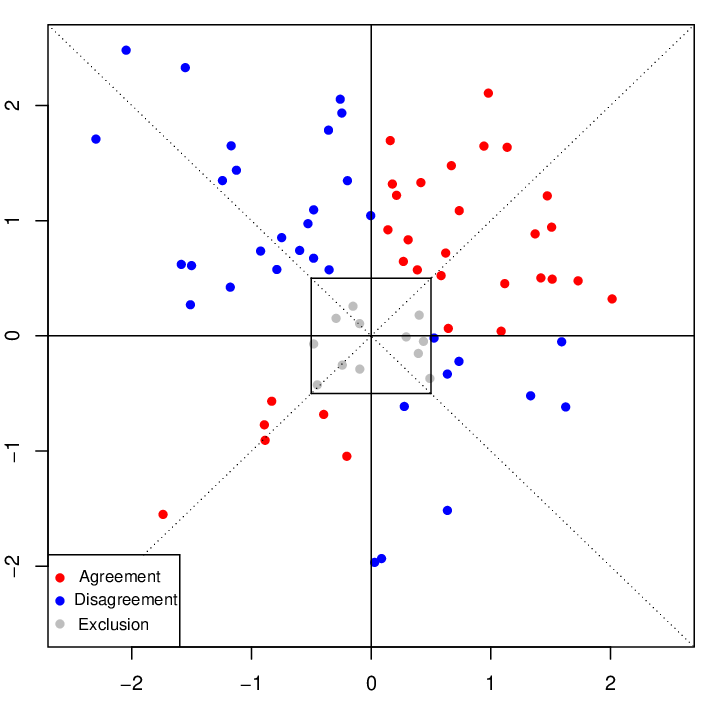
Figure 2 is a four-quadrant plot with artificial example data. In the figure, the red points in the upper-right and lower-left sections are counted as being in “agreement." The blue dots, on the other hand, signify “disagreement." When the difference value of the experimental technique is equal to that of the gold standard, the data dot is on the $45^{\circ}$ lines (dotted lines in Figure 2).

The concordance rate is calculated based on the idea above. The conventional concordance rate (CCR) is defined as follows:

\displaystyle{\rm CCR}(a)=\frac{\#{\rm SA}-\#{\rm AEz}(a)}{nT-\#{\rm Ez}(a)},

(1)

where

	$\displaystyle{\rm SA}=$	$\displaystyle\{(x_{it},y_{it})\|\;{\big(}(x_{it}\geq 0,\;y_{it}\geq 0)\ \cup\ (x_{it}<0,\;y_{it}<0){\big)},$
		$\displaystyle i=1,2,\cdots,n;\;t=1,2,\cdots,T\},$
	$\displaystyle{\rm AEz}(a)=$	$\displaystyle\{(x_{it},y_{it})\|\;{\big(}(0\leq x_{it}\leq a,\;0\leq y_{it}\leq a)\ \cup\ (-a<x_{it}<0,\;-a<y_{it}<0){\big)}$
		$\displaystyle i=1,2,\cdots,n;\;t=1,2,\cdots,T\},\quad{\rm and}$
	$\displaystyle{\rm Ez}(a)=$	$\displaystyle\{(x_{it},y_{it})\|\;-a\leq x_{it},x_{it}\leq a,\;-a\leq y_{it},y_{it}\leq a,\;t=1,2,\cdots,T\}.$

SA is the set of “agreement" pairs of each difference between the values of the gold standard and experimental technique. ${\rm Ez}(a)$ is the set of pairs plotted in the exclusion zone. In the four-quadrant plot, the exclusion zone (middle square in Figure 2) is usually placed to remove data plots close to the origin of the plot, because it is difficult to determine whether such small values have occurred due to the examination or mechanical errors (e.g.,Critchley et al., 2010). The gray points plotted in the exclusion zone in Figure 2 are excluded when calculating the concordance rate. The range of the exclusion zone depends on $a$ , which is set from a clinical point of view (e.g.,Saugel et al., 2015). ${\rm AEz}(a)$ is the set of the “agreement" pairs in the exclusion zone. # signifies the cardinality of a set. The concordance rate in Eq. (1) is the ratio between the number of data points in the “agreement" sections except exclusion zone with all data points that fall outside the exclusion zone.

This conventional concordance rate simply counts the number of data points that show the same trend of change. However, multiple measurements are generally taken for a single patient in a clinical setting. Individual tendencies may influence the measurement results for a single subject. Therefore, individuals must be considered to calculate a more precise concordance rate.

3 Concordance Rate for the Four-quadrant Plot

3.1 General framework of the proposed concordance rate

The proposed concordance rate evaluates the equivalence between the experimental technique and the gold standard through calculation that considers the individual subjects. This proposed method includes the exclusion zone as well, and is defined as the conditional probability, which corresponds to the event falling out of the exclusion zone in all time points. We estimate the parameters of the population with all the data.

The approach for calculation of the proposed method starts with the four-quadrant plot per point $t$ . First, the quadrant sections are named $A_{t}$ to $D_{t}$ . The sample space where the $t$ th value falls in each section can be described in four ways:

	$\displaystyle A_{t}=$	$\displaystyle\{\omega\|\;X_{t}(\omega)\geq 0,Y_{t}(\omega)\geq 0\},$
	$\displaystyle B_{t}=$	$\displaystyle\{\omega\|\;X_{t}(\omega)<0,Y_{t}(\omega)<0\},$
	$\displaystyle C_{t}=$	$\displaystyle\{\omega\|\;X_{t}(\omega)<0,Y_{t}(\omega)\geq 0\},\quad{\rm and}$
	$\displaystyle D_{t}=$	$\displaystyle\{\omega\|\;X_{t}(\omega)\geq 0,Y_{t}(\omega)<0\}\quad(t=1,2,\cdots,T).$

Here, $X_{t}$ and $Y_{t}$ are random variables of each difference of the values of the gold standard and experimental techniques, respectively. $X_{t}$ and $Y_{t}$ correspond to $x_{it}$ and $y_{it}$ , respectively. ${\rm X}=(X_{1},X_{2},\cdots,X_{T})$ and ${\rm Y}=(Y_{1},Y_{2},\cdots,Y_{T})$ are assumed to be distributed from multivariate normal distributions. $A_{t}$ in the upper-right and $B_{t}$ in the lower-left quadrants of the four-quadrant plot (Figure 2) correspond with “agreement," whereas $C_{t}$ in the upper-left and $D_{t}$ in the lower-right quadrants are in “disagreement."

Here, the family of sets is defined as follows:

\displaystyle\mathscr{W}_{t}=\{A_{t}\cup B_{t},C_{t}\cup D_{t}\}\quad(t=1,2,\cdots,T).

Then, exclusion zone at the $t$ th time is

\displaystyle{\rm Ez_{t}}(a)=

\displaystyle\{\omega|\;-a\leq X_{t}(\omega)\leq a,-a\leq Y_{t}(\omega)\leq a\}\quad(t=1,2,\cdots,T).

${\rm Ez}(a)$ is also divided into four-quadrant sections:

	$\displaystyle{\rm EzA_{t}}(a)=$	$\displaystyle\{\omega\|\;0\leq X_{t}(\omega)\leq a,0\leq Y_{t}(\omega)\leq a\},$
	$\displaystyle{\rm EzB_{t}}(a)=$	$\displaystyle\{\omega\|\;-a\leq X_{t}(\omega)\leq 0,-a\leq Y_{t}(\omega)\leq 0\},$
	$\displaystyle{\rm EzC_{t}}(a)=$	$\displaystyle\{\omega\|\;-a\leq X_{t}(\omega)\leq 0,0\leq Y_{t}(\omega)\leq a\},$
	$\displaystyle{\rm EzD_{t}}(a)=$	$\displaystyle\{\omega\|\;0\leq X_{t}(\omega)\leq a,-a\leq Y_{t}(\omega)\leq 0\}\quad(t=1,2,\cdots,T).$

The assets of the random variables in $A_{t},B_{t},C_{t}$ , and $D_{t}$ , except the exclusion zone, are defined as follows:

	$\displaystyle A_{t}^{\dagger}=$	$\displaystyle A_{t}\cap{\rm EzrA_{t}}(a)^{c},$
	$\displaystyle B_{t}^{\dagger}=$	$\displaystyle B_{t}\cap{\rm EzrB_{t}}(a)^{c},$
	$\displaystyle C_{t}^{\dagger}=$	$\displaystyle C_{t}\cap{\rm EzrC_{t}}(a)^{c},\quad{\rm and}$
	$\displaystyle D_{t}^{\dagger}=$	$\displaystyle D_{t}\cap{\rm EzrD_{t}}(a)^{c},$

where $Z^{c}$ is the complement of arbitrary set $Z$ . $A_{t}^{\dagger}$ and $B_{t}^{\dagger}$ are the events of “agreement" that do not fall into the exclusion zone, whereas $C_{t}^{\dagger}$ and $D_{t}^{\dagger}$ are the events of “disagreement" out of the exclusion zone.

The proposed concordance rate is calculated in the condition when all pairs of $(X_{t},Y_{t})$ are not in the exclusion zone. This means that all data of one subject are excluded from the calculation if any pair of data points for that subject drops to the exclusion zone at least once. This can be described as

\displaystyle{\rm NEz(a)}=\Big\{\omega|\;\forall t\;(t=1,2,\cdots,T);\;\omega\notin{\rm Ez}_{t}(a)\Big\}.

Here, the two clinical testing methods are regarded as equivalent if $X_{t}$ and $Y_{t}$ show the same direction of trends more than $m$ times out of $T$ times per subject. Concordance rate in the agreement times more than the setting number in $m$ is calculated. $m$ is determined from a clinical perspective. $T$ is the number of differences of measurement values. Given this idea, we propose the new concordance rate, wherein the probability of “agreement" of more than $m$ times in $T$ is defined as follows:

	$\displaystyle P\Big[\bigcup_{t=m}^{T}H_{t}\|{\rm NEz}(a)\Big]\ =$	$\displaystyle\frac{P\Big[(\bigcup_{t=m}^{T}H_{t})\cap{\rm NEz}(a)\Big]}{P\Big[{\rm NEz}(a)\Big]}$
	$\displaystyle=$	$\displaystyle\frac{\sum_{t=m}^{T}P\Big[H_{t}\cap{\rm NEz}(a)\Big]}{1-P\Big[\bigcup_{s=1}^{T}{\rm Ez_{s}}(a)\Big]},$		(2)

where

\displaystyle H_{t}=\Big\{\omega|\;(W_{1}(\omega),W_{2}(\omega),\cdots,W_{T}(\omega))\in\prod_{s=1}^{T}\mathscr{W}_{s},\sum_{s=1}^{T}I(W_{s}(\omega)=A_{s}(\omega)\cup B_{s}(\omega))=t\Big\}.

(3)

$H_{t}$ in Eq. (2) is the subset of the sample space wherein the trend between $X$ and $Y$ agrees $t$ times. $I$ is the indicator function in the condition wherein the $s$ th data fall in $A^{\dagger}$ or $B^{\dagger}$ . $\prod_{s=1}^{T}\mathscr{W}_{s}$ in Eq. (3) indicates the product.

3.2 Example of the proposal index, T = 2

Next, we explain the proposed concordance rate in the case of $m=1$ and $T=2$ , that is, at three points in time. The probability can be calculated as follows:

\displaystyle P\Big[\Big(\bigcup_{t=1}^{2}H_{t}\Big)\cap{\rm NEz}(a)\Big]\ =\frac{\sum_{t=1}^{2}P\Big[H_{t}\cap{\rm NEz}(a)\Big]}{1-P\Big[\bigcup_{s=1}^{2}{\rm Ez}_{s}(a)\Big]}.

(4)

We apply the definition at $T=2$ to a four-quadrant plot. There are three patterns in the case of $T=2$ : agreement in $t=1$ , agreement in $t=2$ , and agreements in $t=1$ and $t=2$ . The probability of the numerator in the definition formula is

	$\displaystyle P[H_{1}\cap{\rm NEz}(a)]=$	$\displaystyle P[(A_{1}^{\dagger}\cup B_{1}^{\dagger})\cap(C_{2}^{\dagger}\cup D_{2}^{\dagger})]+P[(C_{1}^{\dagger}\cup D_{1}^{\dagger})\cap(A_{2}^{\dagger}\cup B_{2}^{\dagger})]$		(5)
	$\displaystyle P[H_{2}\cap{\rm NEz}(a)]=$	$\displaystyle P[(A_{1}^{\dagger}\cup B_{1}^{\dagger})\cap(A_{2}^{\dagger}\cup B_{2}^{\dagger})].$		(6)

To describe each case, the range wherein the data point enters into each quadrant of the plot is set as $F=\{[0,\infty]^{T},\;[-\infty,0]^{T}\}$ , and the range of the exclusion zone is $E=\{[0,a]^{T},\;[-a,0]^{T}\}$ . Vectors to describe the range for the probability calculations are as follows:

\displaystyle{\bf v_{1}}=\left[\begin{array}[]{c}v_{11}\\ v_{21}\\ \end{array}\right],\quad{\bf v_{2}}=\left[\begin{array}[]{c}v_{12}\\ v_{22}\\ \end{array}\right],\quad{\bf z_{1}}=\left[\begin{array}[]{c}z_{11}\\ z_{21}\\ \end{array}\right],\quad{\bf z_{2}}=\left[\begin{array}[]{c}z_{12}\\ z_{22}\\ \end{array}\right].

The first term of Eq. (5) means the probability with which the trend of $X_{1}$ and $Y_{1}$ is in agreement, whereas that of $X_{2}$ and $Y_{2}$ is not. This can also be expressed as

		$\displaystyle P\Big[(A_{1}^{\dagger}\cup B_{1}^{\dagger})\cap(C_{2}^{\dagger}\cup D_{2}^{\dagger})\Big]$
	$\displaystyle=$	$\displaystyle\sum_{\begin{subarray}{c}{\bf v_{1}}={\bf z_{1}},{\bf v_{2}}\neq{\bf z_{2}}\\ {\bf v_{1}},{\bf v_{2}},{\bf z_{1}},{\bf z_{2}}\in F\end{subarray}}P(v_{11}<X_{1}<v_{21},\;v_{12}<X_{2}<v_{22},\;z_{11}<Y_{1}<z_{21},\;z_{12}<Y_{2}<z_{22})$
		$\displaystyle+\sum_{\begin{subarray}{c}{\bf v_{1}}={\bf z_{1}},{\bf v_{2}}\neq{\bf z_{2}}\\ {\bf v_{1}},{\bf v_{2}},{\bf z_{1}},{\bf z_{2}}\in E\end{subarray}}P(v_{11}<X_{1}<v_{21},\;v_{12}<X_{2}<v_{22},\;z_{11}<Y_{1}<z_{21},\;z_{12}<Y_{2}<z_{22})$
		$\displaystyle-\sum_{\begin{subarray}{c}{\bf v_{1}}={\bf z_{1}},{\bf v_{2}}\neq{\bf z_{2}}\\ {\bf v_{1}},{\bf z_{1}}\in F,\;{\bf v_{2}},{\bf z_{2}}\in E\end{subarray}}P(v_{11}<X_{1}<v_{21},\;v_{12}<X_{2}<v_{22},\;z_{11}<Y_{1}<z_{21},\;z_{12}<Y_{2}<z_{22})$
		$\displaystyle-\sum_{\begin{subarray}{c}{\bf v_{1}}={\bf z_{1}},{\bf v_{2}}\neq{\bf z_{2}}\\ {\bf v_{1}},{\bf z_{1}}\in E,\;{\bf v_{2}},{\bf z_{2}}\in F\end{subarray}}P(v_{11}<X_{1}<v_{21},\;v_{12}<X_{2}<v_{22},\;z_{11}<Y_{1}<z_{21},\;z_{12}<Y_{2}<z_{22}).$

Then, the second term of Eq. (5) is the probability when the trend of $X_{1}$ and $Y_{1}$ is in disagreement, but that of $X_{2}$ and $Y_{2}$ is in agreement. This can be rewritten similarly as

		$\displaystyle P\Big[(C_{1}^{\dagger}\cup D_{1}^{\dagger})\cap(A_{2}^{\dagger}\cup B_{2}^{\dagger})\Big]$
	$\displaystyle=$	$\displaystyle\sum_{\begin{subarray}{c}\bf{v}_{1}\neq{\bf z_{1}},{\bf v_{2}}={\bf z_{2}}\\ {\bf v_{1}},{\bf v_{2}},{\bf z_{1}},{\bf z_{2}}\in F\end{subarray}}P(v_{11}<X_{1}<v_{21},\;v_{12}<X_{2}<v_{22},\;z_{11}<Y_{1}<z_{21},\;z_{12}<Y_{2}<z_{22})$
		$\displaystyle+\sum_{\begin{subarray}{c}{\bf v_{1}}\neq{\bf z_{1}},{\bf v_{2}}={\bf z_{2}}\\ {\bf v_{1}},{\bf v_{2}},{\bf z_{1}},{\bf z_{2}}\in E\end{subarray}}P(v_{11}<X_{1}<v_{21},\;v_{12}<X_{2}<v_{22},\;z_{11}<Y_{1}<z_{21},\;z_{12}<Y_{2}<z_{22})$
		$\displaystyle-\sum_{\begin{subarray}{c}{\bf v_{1}}\neq{\bf z_{1}},{\bf v_{2}}={\bf z_{2}}\\ {\bf v_{1}},{\bf z_{1}}\in F,\;{\bf v_{2}},{\bf z_{2}}\in E\end{subarray}}P(v_{11}<X_{1}<v_{21},\;v_{12}<X_{2}<v_{22},\;z_{11}<Y_{1}<z_{21},\;z_{12}<Y_{2}<z_{22})$
		$\displaystyle-\sum_{\begin{subarray}{c}{\bf v_{1}}\neq{\bf z_{1}},{\bf v_{2}}={\bf z_{2}}\\ {\bf v_{1}},{\bf z_{1}}\in E,\;{\bf v_{2}},{\bf z_{2}}\in F\end{subarray}}P(v_{11}<X_{1}<v_{21},\;v_{12}<X_{2}<v_{22},\;z_{11}<Y_{1}<z_{21},\;z_{12}<Y_{2}<z_{22}).$

Eq. (6) is the probability that the trends of $X_{1}$ and $Y_{1}$ and of $X_{2}$ and $Y_{2}$ are both concordant:

		$\displaystyle P\Big[(A_{1}^{\dagger}\cup B_{1}^{\dagger})\cap(A_{2}^{\dagger}\cup B_{2}^{\dagger})\Big]$
	$\displaystyle=$	$\displaystyle\sum_{\begin{subarray}{c}{\bf v_{1}}={\bf z_{1}},{\bf v_{2}}={\bf z_{2}}\\ {\bf v_{1}},{\bf v_{2}},{\bf z_{1}},{\bf z_{2}}\in F\end{subarray}}P(v_{11}<X_{1}<v_{21},\;v_{12}<X_{2}<v_{22},\;z_{11}<Y_{1}<z_{21},\;z_{12}<Y_{2}<z_{22})$
		$\displaystyle+\sum_{\begin{subarray}{c}{\bf v_{1}}={\bf z_{1}},{\bf v_{2}}={\bf z_{2}}\\ {\bf v_{1}},{\bf v_{2}},{\bf z_{1}},{\bf z_{2}}\in E\end{subarray}}P(v_{11}<X_{1}<v_{21},\;v_{12}<X_{2}<v_{22},\;z_{11}<Y_{1}<z_{21},\;z_{12}<Y_{2}<z_{22})$
		$\displaystyle-\sum_{\begin{subarray}{c}{\bf v_{1}}={\bf z_{1}},{\bf v_{2}}={\bf z_{2}}\\ {\bf v_{1}},{\bf z_{1}}\in F,\;{\bf v_{2}},{\bf z_{2}}\in E\end{subarray}}P(v_{11}<X_{1}<v_{21},\;v_{12}<X_{2}<v_{22},\;z_{11}<Y_{1}<z_{21},\;z_{12}<Y_{2}<z_{22})$
		$\displaystyle-\sum_{\begin{subarray}{c}{\bf v_{1}}={\bf z_{1}},{\bf v_{2}}={\bf z_{2}}\\ {\bf v_{1}},{\bf z_{1}}\in E,\;{\bf v_{2}},{\bf z_{2}}\in F\end{subarray}}P(v_{11}<X_{1}<v_{21},\;v_{12}<X_{2}<v_{22},\;z_{11}<Y_{1}<z_{21},\;z_{12}<Y_{2}<z_{22}).$

Finally, the probability of the denominator in $T=2$ is

		$\displaystyle 1-P\Big[\bigcup_{s=1}^{2}{\rm Ez}_{s}(a)\Big]$
	$\displaystyle=$	$\displaystyle 1-P(-a<X_{1}<a.-\infty<X_{2}<\infty,\;-a<Y_{1}<a,-a<Y_{2}<a)$
		$\displaystyle-P(-\infty<X_{1}<\infty,-a<X_{2}<a,\;-\infty<Y_{1}<\infty,-a<Y_{2}<a)$
		$\displaystyle+P(-a<X_{1}<a,-a<X_{2}<a,\;-a<Y_{1}<a,-a<Y_{2}<a).$

In the proposed concordance rate, we assume that all random variables are distributed from multivariate normal distribution. Therefore, we must estimate the mean vectors and covariance matrices to calculate the concordance rate. The method of estimating these parameters is described next.

3.3 Estimation

First, we define $Z=(X_{1},\;\cdots,\;X_{T},\;Y_{1},\;\cdots,\;Y_{T})=(Z_{1},\;\cdots,\;Z_{T},Z_{T+1},\;\cdots,\;Z_{T+T})$ . Since the proposed method assumes that $Z$ are distributed from $T+T$ -dimensional normal distributions, it is necessary to estimate the $T+T$ -dimensional mean vector and variance covariance matrix to calculate the concordance rate. The estimated mean vector in the proposed approach is $\bar{\bm{z}}=(\bar{x}_{1},\;\cdots,\;\bar{x}_{T},\;\bar{y}_{1},\;\cdots,\;\bar{y}_{T})^{T}$ , where $\bar{x}_{t}$ and $\bar{y}_{t}$ are the mean of the $t$ th value of gold standard and experimental technique, respectively. The covariance matrix based on the differences between the times is ${\bm{S}}=(s_{tk})\quad(t,k=1,2,\cdots,T+T)$ , where $s_{tk}$ is the covariance between $t$ and $k$ . By using these estimator, the proposed concordance rate in Eq (2), defined as the conditional probability, can be calculated.

4 Numerical Simulation

In this section, we describe the simulation design, and present the simulation results. We conducted a simulation and set the two types of evaluation for the simulation. First, we examined how close the concordance rates calculated with the conventional methods and the proposed approach were to the result of the true concordance rate. The assessment of each concordance rate was expressed as the difference from the true concordance rate. The results of the proposed method can not be simply compared with CCR $(a)$ , since CCR $(a)$ does not consider the repeated measurement. In order to compare with the conventional concordance rate, control1 and control2 were adjusted to allow repeated measurements, which details in factor 7. Secondly, to compare the diagnosability of the proposed method with CCR $(a)$ , we calculated ROC curves and Area Under the Curve (AUC) (e.g. Pepe, 2003). The second evaluation is based on AUC. In this simulation, we used RStudio Version 1.1.453.

4.1 Simulation design

We set $T=2$ , and the data generation procedure is as follows:

\displaystyle\bf{Z}\sim N(\bf{\mu}_{z},\Sigma_{z})

where ${\bf Z}=(X_{1},X_{2},Y_{1},Y_{2})^{T}$ . $X_{t}$ is the difference in the measurement values of the gold standard between the $t$ th and $(t+1)$ th times $(t=1,2,3)$ , and $Y_{t}$ is that of experimental technique.

In addition,

\displaystyle\bm{\mu}_{Z}=\left[\begin{array}[]{c}\bm{\mu}_{X}\\ \bm{\mu}_{Y}\\ \end{array}\right],\quad\bm{\Sigma}_{Z}=\left[\begin{array}[]{cc}\bm{\Sigma}_{X}&\bm{\Sigma}_{XY}\\ \bm{\Sigma}_{XY}&\bm{\Sigma}_{Y}\\ \end{array}\right],

where $\bf{\mu}_{X}=(\mu_{x1},\mu_{x2})^{T}$ and $\bf{\mu}_{Y}=(\mu_{y1},\mu_{y2})^{T}$ are the mean vectors of the gold standard and experimental technique, and $\bf{\Sigma}_{X}$ and $\bf{\Sigma}_{Y}$ are the covariance matrices, respectively.
Here,

\displaystyle\bm{\Sigma}_{X}=\left[\begin{array}[]{cc}{\sigma}_{x1}&{\rho}\\ {\rho}&{\sigma}_{x2}\\ \end{array}\right],\quad\bm{\Sigma}_{Y}=\left[\begin{array}[]{cc}{\sigma}_{y1}&{\rho}\\ {\rho}&{\sigma}_{y2}\\ \end{array}\right],\ {\rm and}\ \quad\bm{\Sigma}_{XY}=\left[\begin{array}[]{cc}{\rho}_{XY}&{\rho}_{XY}\\ {\rho}_{XY}&{\rho}_{XY}\\ \end{array}\right].

we set $\sigma_{x1}=\sigma_{x2}=\sigma_{y1}=\sigma_{y2}=1$ .

Factors set in the simulation are presented in Table 1. The number of total patterns is $30\times 3\times 2\times 2\times 2\times 2\times 3=4320$ . For each pattern, corresponding artificial data are generated 100 times and we evaluate the results. The levels of the seven factors are set as follows.

Factor 1: Means

The mean is of 30 patterns, as shown in Table 2. The setting depends on the combination of the magnitude of the mean value and the direction of change in $x$ and $y$ .

Factor 2: Covariance between the difference values within each measurement method

The corvariance within each measurement method of the difference values, ${\rho}$ , is set as $0$ , $1/3$ and $2/3$ in both $X$ and $Y$ .

Factor 3: Covariance between $X$ and $Y$

${\rho}_{XY}=0$ and $1/3$ .

Factor 4: Number of agreements

Factor 4 is the number of trending agreements between $X$ and $Y$ . We set two different situations: (1) agreement more than once in $T=2$ , and (2) agreement at both time points.

Factor 5: Exclusion zone

$a$ of the exclusion zone ${\rm Ez}(a)$ is set as 0.5 and 1.0.

Factor 6: Number of subjects

The number of subjects is set as 15 and 40.

Factor 7: Methods

We calculate the concordance rate by four methods. Control1, control2, and the proposed method are used in the first evaluation, and CCR, Control1, control2, and the proposed method are used in the second evaluation. We denote the proposed concordance rate as “proposal".

Control1, based on binomial distribution, is calculated as follows:

\displaystyle\sum_{s=m}^{2}{}_{2}C_{s}p^{s}(1-p)^{(2-s)},

where

\displaystyle p=\frac{k_{1}+k_{2}}{n_{1}^{\dagger}+n_{2}^{\dagger}}.

${k_{t}}$ ( $t=1,2$ ) is the number of data that show the same trend between $X_{t}$ and $Y_{t}$ out of the exclusion zone. $n_{t}^{\dagger}$ is the number of subjects whose data points fall out of the exclusion zone. The concordance rate in control2 is calculated by the probability at each number of agreement: twice in two time points is $p_{1}p_{2}$ , and once in two time points $p_{1}(1-p_{2})+(1-p_{1})p_{2}$ ,

where

\displaystyle p_{t}=\frac{k_{t}}{n_{t}^{\dagger}}\quad(t=1,2).

Subjects whose difference value fall in the exclusion zone of the four-quadrant plot even once are excluded from the calculation of the concordance rate in both control1 and control2 as same manner of the proposed method.

The first evaluation index for the simulation result is the absolute values of the difference between the concordance rate based on each estimated parameters and the concordance rate computed with the true mean vector $\bm{\mu}_{Z}$ and with true covariance matrix $\bm{\Sigma}_{Z}$ . We set the evaluation to deserve as better assessment if the absolute values of the difference between the true value and the estimated values are smaller among all concordance rate approaches.

For the second evaluation index, we label to each pattern of means in Table 1. If $\bf{\mu}_{X}$ and $\bf{\mu}_{Y}$ are concordant both two times, we mark the corresponding mean pattern as “ $\circ$ ", and the rest as “ $\times$ ". Then, the 4320 $\times$ 100 data in total have this label. ROC and AUC (e.g. Pepe, 2003) are calculated by the label and the results of concordance rates in each method, and we compare these results of AUC among the proposal method, CCR $(a)$ , control1 and control2.

Table 1: Factors of the simulation design

Factor No.	Factor name	levels
Factor 1	Means	30
Factor 2	Covariance between the difference values within each measurement method	3
Factor 3	Covariance between $X$ and $Y$	2
Factor 4	Number of agreements	2
Factor 5	Exclusion zone	2
Factor 6	Number of subjects	2
Factor 7	Methods	3 / 4

Table 2: Mean patterns in Factor 1: Label

\circ

indicates the pattern of agreement between

\mu_{X}

and

\mu_{Y}

2 times,

\times

indicates the pattern of not agreement between

\mu_{X}

and

\mu_{Y}

2 times

Pattern No.	$\mu_{X1}$	$\mu_{X2}$	$\mu_{Y1}$	$\mu_{Y2}$	Label	Pattern No.	$\mu_{X1}$	$\mu_{X2}$	$\mu_{Y1}$	$\mu_{Y2}$	Label
Pattern1	-1.5	-1.5	1.5	1.5	$\times$	Pattern16	0.5	0.5	-0.5	-0.5	$\times$
Pattern2	-0.5	-0.5	0.5	0.5	$\times$	Pattern17	-0.5	-1.5	-0.5	-1.5	$\circ$
Pattern3	-1.5	1.5	1.5	1.5	$\times$	Pattern18	0.5	-1.5	-0.5	-1.5	$\times$
Pattern4	0.5	-0.5	0.5	0.5	$\times$	Pattern19	-0.5	1.5	-0.5	-1.5	$\times$
Pattern5	1.5	1.5	1.5	1.5	$\circ$	Pattern20	0.5	1.5	-0.5	-1.5	$\times$
Pattern6	0.5	0.5	0.5	0.5	$\circ$	Pattern21	-1.5	-1.5	-1.5	1.5	$\times$
Pattern7	-0.5	-1.5	0.5	1.5	$\times$	Pattern22	-0.5	-0.5	-0.5	0.5	$\times$
Pattern8	0.5	-1.5	0.5	1.5	$\times$	Pattern23	-1.5	1.5	-1.5	1.5	$\circ$
Pattern9	-0.5	1.5	0.5	1.5	$\times$	Pattern24	0.5	-0.5	-0.5	0.5	$\times$
Pattern10	0.5	1.5	0.5	1.5	$\circ$	Pattern25	1.5	1.5	-1.5	1.5	$\times$
Pattern11	-1.5	-1.5	-1.5	-1.5	$\circ$	Pattern26	0.5	0.5	-0.5	0.5	$\times$
Pattern12	-0.5	-0.5	-0.5	-0.5	$\circ$	Pattern27	-0.5	-1.5	-0.5	1.5	$\times$
Pattern13	-1.5	1.5	-1.5	-1.5	$\times$	Pattern28	0.5	-1.5	-0.5	1.5	$\times$
Pattern14	0.5	-0.5	-0.5	-0.5	$\times$	Pattern29	-0.5	1.5	-0.5	1.5	$\circ$
Pattern15	1.5	1.5	-1.5	-1.5	$\times$	Pattern30	0.5	1.5	-0.5	1.5	$\times$

4.2 Simulation results

4.2.1 Difference between the true value and the estimation of each concordance rate method

In all simulation results, the proposed approach was closer to the true value than control methods. Figure 3 showed the result of this simulation. We also showed median, the first quartile and the third quartile by each factor in tables. Medians of the proposal method was smaller, and the interquantile range was narrower than than the control1 and control2 in all factors. These results indicate that the variation of the proposed method was smaller than two control concordance methods. The estimation of the proposal was stable. Table 3 are the results par each pattern of the mean. In Pattern3, 13, 21 and 25, the bias of control1 tended to be large. These patterns are the situation that the all absolute values of means of $X$ and $Y$ are 1.5 and the direction of trends disagree two times. compared to the control methods, the proposed method was stable in all patterns. Table 4 is the results of the covariance of the difference values within each measurement method and table 5 is the results of the covariance between $X$ ans $Y$ . The results of all methods were almost same in terms of both covariances. The proposed method was more stable than the conventional methods in both factors. The proposed method resulted more closely to the true values in both $m=1$ and $m=2$ than the control methods (Table 6). It means that the proposal evaluated more properly in all number of agreement in the case of $T=2$ . Regarding the exclusion zone, the concordance rates was slightly higher in larger size of the exclusion zone (Table 7). The concordance rates in all methods were smaller in the larger number of subjects (Table 9).

4.2.2 Diagnosability of the estimation of each concordance method

To compare the diagnosability of the proposed method with that of the conventional methods, we described the ROC curves of the proposal, CCR, control1 and control2 in Figure 4 and calculated their AUC in Table 9. Seeing from the results of AUC, the proposed method was better than the conventional methods. In other words, it showed that the diagnostic capability of the proposed method was superior to the conventional methods.

References

- [1] Altman, D. and Bland, J. (1983) Measurement in medicine: the analysis of method comparison studies. Journal of the Royal Statistical Society. Series D (The Statistician), 32(3), 307–317.
- [2] Altman D.G, and Bland J.M. (1991) The analysis of blood pressure data. In O’Brien E, O’Malley K eds. Blood pressure measurement, 287–314.
- [3] Asamoto, M., Orii, R., Otsuji, M, Bougaki, M., Imai, Y. and Ymada, Y. (2017) Reliability of cardiac output measurements using lidcorapidTM and flotrac/vigileoTM across broad ranges of cardiac output values. Journal of clinical monitoring and computing, 31(4), 709–716.
- [4] Bartko, J. (1976) Agreement between methods of measurement with multiple observations per individual. Psychological Bulletin, 83(5), 762–765.
- [5] Bland, J. and Altman (1986) Statistical methods for assessing agreement between two methods of clinical measurement. The lancet, 327(8476), 307–310.
- [6] Bland, J. and Altman (1999) Measuring agreement in method comparison studies. Statistical methods in medical research, 8(2), 135–160.
- [7] Bland, J. and Altman (2007) Agreement between methods of measurement with multiple observations per individual. Journal of biopharmaceutical statistics, 17(4), 571–582.
- [8] Carstensen, B. (2010) Comparing Clinical Measurement Methods a practical guide, John Wiley Sonsl.
- [9] Carstensen, B., Gurrin, L., Ekstrom, C. T. and Figurski, M. (2020) Methcomp: Analysis of agreement in method comparison studies. https://CRAN.Rproject. org/package=MethComp.
- [10] Choudhary, P. and Nagaraja, H. (2017) Measuring Agreement; Models, Methods, and Applications, John Wiley Sonsl.
- [11] Choundhary, P., and Nagaraja, H.(2005) Assessment of agreement using intersection-union principle. Biometrical Journal, 47(5), 674–681.
- [12] Cox, P., den Ouden, A., Theunissen, M., Montenij, L., Kessels, A., Lanc’e, Buhre, W. and Marcus, M.A.E.(2017) Accuracy, precision, and trending ability of electrical cardiometry cardiac index versus continuous pulmonary artery thermodilution method: A prospective, observational study. Measuring Agreement; Models, Methods, and Applications, BioMed Research International, 2635151.
- [13] Critchley, L. A., Lee, A. and Ho, A. M.-H. (2010) A critical review of the ability of continuous cardiac output monitors to measure trends in cardiac output. Anesth. Analg, 111(5), 1180–1192.
- [14] Critchley, L. A., Yang, X. X. and Lee, A. (2011) Assessment of trending ability of cardiac output monitors by polar plot methodology. Journal of Cardiothoracic and Vascular Anesthesia, 25(3), 536–546.
- [15] Goodman, L.A. and Kruskal, W.H. (1963) Measures of association for cross classifications III: approximate sampling theory. Journal of the American Statistical Association, 58(302), 310–364.
- [16] Monnet, X., Anguel, N., Jozwiak, M., Richard, C. and Teboul, J.-L.(2012) Thirdgeneration flotrac/vigileo does not reliably track changes in cardiac output induced by norepinephrine in critically ill patients. British Journal of Anaesthesia, 108(4), 615–622.
- [17] Pepe, M. S. (2003) The Statistical Evaluation of Medical Tests for Classification and Prediction. Oxford: Oxford University Press.
- [18] Perrino, A. J., Harris, S. and Luther, M.(1998) Intraoperative determination of cardiac output using multiplane transesophageal echocardiography : A comparison to thermodilution. Anesthesiology, 89(8), 350–357.
- [19] Perrino, A. J., O’Connor, T. and Luther, M.(1994) Transtracheal doppler cardiac output monitoring: Comparison to thermodilution during noncardiac surgery. Anesthesia Analgesia, 78(6), 1060–1066.
- [20] Saugel, B., Grothe, O. and Wagner, J.(2015) Tracking changes in cardiac output: Statistical considerations on the 4-quadrant plot and the polar plot methodology. Anesthesia Analgesia, 121(2), 514–524.
- [21] Shieh, G. (2019) Assessing agreement between two methods of quantitative measurements. Statistics in Biopharmaceutical Research, Online.
- [22] Zou, G. (2013) Confidence interval estimation for the bland-altman limits of agreement with multiple observations per individual. Statistical methods in medical research, 22(6), 630–642.