Secure Distributed Matrix Computation with Discrete Fourier Transform

The cryptography community has extensively studied the problem of secure multi-party computation (MPC), also known as secure function evaluation, in which Alice and Bob, having inputs $x$ and $y$, respectively, want to compute a function $f(x,y)$ jointly, without any of them learning anything about the other’s input either from the communication, or from the result of the computation [1]. The SDMM problem is related to MPC yet different; the design has to ensure that no computing server learns anything about the original data, but we can decide which part of the data is revealed to each server and in what form. Fully homomorphic encryption (FHE) is a class of cryptographic schemes that allow computations on ciphertexts, generating an encrypted result which, when decrypted, matches the result of the operations as if they had been performed on plaintext. These techniques rely on working over polynomial rings, and their security is based on the assumed (or proven) hardness of problems in ideal lattices [2, 3]. However, existing FHE schemes are slow and impractical. “Somewhat homomorphic encryption” (SHE) has been proposed as an alternative, which allows a limited number of homomorphic operations on ciphertexts. SHE is relatively faster, and ciphertext packing methods have been proposed for operations like secure inner products [2, 4], and secure matrix multiplications [3], which generalizes Yasuda et al.’s packing method for inner products in [4]. Some works also propose methods for performing other matrix computations in an information theoretically secure manner, like Gaussian elimination, matrix inversion, comparison, equality test, or exponentiation [5, 6].

There is also a growing literature on distributed matrix multiplication, where a lot of effort has been put into speeding up computations, increasing reliability, and/or reducing communication overhead using coding and communication theoretic ideas [7, 8, 9, 10, 11, 12, 13]. The initial papers considered a slightly different context of speeding up parallel computations by introducing “computation redundancy” to mitigate the problem of straggling servers [7, 8]. Straggling servers refer to slow/unresponsive servers due to which completion of the computation is delayed. A standard way of dealing with stragglers is to introduce “computation redundancy”, that is, assigning extra computations to each server. In coded computation against stragglers, the performance metric is the recovery threshold; that is, the minimum integer $r$ such that the computation result is recoverable from any $r$ successful (non-delayed, non-faulty) servers. The common theme in the ‘coded computation’ literature is to treat stragglers as ‘erasures’ in communications, and exploit ideas for coding against erasures, which allows reliable reconstruction of the desired result from an arbitrary set of successfully received symbols. Reference [9] uses polynomial codes to construct a scheme in which the computation is completed as long as any $K$ out of $N$ evaluations of a polynomial are received from the servers. To multiply two matrices $\mathbf{A}$ and $\mathbf{B}$ with the help of $N$ servers, the polynomial code in [9] partitions $\mathbf{A}$ row-wise and $\mathbf{B}$ column-wise (row-by-column partitioning), and generates encoded matrices as evaluations of a polynomial with the blocks as the coefficients, similarly to Reed Solomon codes [14]. A follow-up work [10] proposes a new polynomial coded computation scheme called MatDot, which achieves the optimal recovery threshold for column-wise partitioning of matrix $\mathbf{A}$ and row-wise partitioning of $\mathbf{B}$ (sum-of-outer-products method), which we shall refer to as the column-by-row partitioning henceforth in the paper, at the expense of an increase in the communication cost. In [10], the authors also propose PolyDot codes that interpolate between the polynomial codes of [9] and MatDot codes. PolyDot codes are later improved as generalized PolyDot (GPD) codes in [11], which achieve the optimal recovery threshold for any arbitrary partitioning of the input matrices. Entangled polynomial codes, proposed in parallel in [12], also achieve the same performance as GPD codes. Bivariate polynomial codes are introduced in [15] for straggler mitigation when servers can compute and transmit multiple partial computations.

Subsequent papers, inspired by the works on straggler mitigation in distributed matrix multiplication, consider the SDMM problem from an information theoretic perspective. These papers aim for information theoretic security, independent of the computational capacities of the attackers, as opposed to cryptographic techniques. These works typically assume that the data to be used for computations belongs to the user; hence, they focus on privacy against the servers. The earlier papers on SDMM consider download rate as the performance metric, which is defined as the ratio of the number of bits required to represent the computation result to the total number of bits that the servers must transmit to the user. Reference [16] uses the idea of polynomial codes from the literature on straggler mitigation to propose an SDMM scheme based on Shamir’s secret sharing scheme [17], which is shown to achieve the optimal download rate for one-sided SDMM (where only one of the matrices is kept secure). An achievable scheme is also proposed for two-sided SDMM (both matrices are kept secure). Reference [18] introduces GASP codes, which improve the download rate for two-sided SDMM by aligning the degrees of the terms in the polynomial code so that the desired products appear as distinct terms.

In [19], new converse bounds on the optimal download rate for SDMM are obtained by showing that the capacity of a multi-message X-secure T-private information retrieval (MM-XSTPIR) problem ([20, 21]) provides an upper bound on the download rate of the SDMM problem. The optimal download rate of the MM-XSTPIR problem is shown to depend on the dimensions of the matrices $\mathbf{A}$ and $\mathbf{B}$. The scheme in [19] allows the joint retrieval of a batch of matrix products (batch multiplication), instead of multiplying two matrices using the matrix partitioning approach, resulting in a coding gain. Other recent works on secure distributed batch matrix multiplication include [22] and [23].

Reference [13] combines straggler mitigation and secure computation using the batch multiplication approach. Byzantine security is also considered, which refers to security against adversarial servers that may actively corrupt the results they send back to the user. Their scheme is based on Lagrange polynomials, and it achieves the optimal recovery threshold for any multi-linear function computation. Since the scheme in [13] is designed for batch computation of any function, we can adapt it for matrix multiplication using a matrix-partitioning based approach, and compare its performance with that of other matrix partitioning based schemes. This can be done by treating the partitions of the matrices to be multiplied as batches of data. Therefore, if $\mathbf{A}$ is partitioned column-wise and $\mathbf{B}$ is partitioned row-wise into $K$ partitions each, the scheme in [13] has the recovery threshold of $2(K+T-1)+S+2A+1$, where $S$ and $A$ are the numbers of stragglers and Byzantine adversaries, respectively. If $\mathbf{A}$ is partitioned row-wise and $\mathbf{B}$ is partitioned column-wise, into $K$ and $L$ partitions respectively, the recovery threshold is $2(KL+T-1)+S+2A+1$, which is the same performance as that of the GASP codes in [18] for big $T$, which can be seen by setting $S=A=0$. For arbitrary matrix partitions, the Lagrange coded scheme does not perform as well as the secure generalized PolyDot (SGPD) codes introduced later in [24]. In [24], the trade-off between the download rate and the recovery threshold, first studied in [25] using the MatDot and PolyDot schemes for straggler mitigation, is extended to SDMM. The SGPD codes achieve the same recovery threshold as Lagrange codes for the sum-of-outer-products method.

In [26], the trade-off between the upload and download costs for SDMM is studied. While the download cost is simply the reciprocal of the download rate, the upload cost is defined as the ratio of the total number of bits that the user must send to the servers to the total size in bits of the data matrices. In [26], a secure cross subspace alignment (SCSA) scheme with adjustable upload cost (USCSA) is presented for SDMM. The tradeoff between the upload and download costs for SDMM schemes using only the row-by-column partitioning is studied in [26], but not the tradeoff for SDMM schemes using the column-by-row partitioning.

The work that is most related to ours is [27], which considers the setting in which the data is generated at distributed source nodes, and does not belong to the user requesting the computation. It extends the BGW (Ben-Or, Goldwasser and Widgerson) scheme from [28], which was first proposed in the context of secure MPC, for multiplication of matrices using a connected network of computing servers. The sources are assumed not to be connected with each other, while the servers are. The latter assumption is exploited to reduce the communication to the user by allowing the servers to cooperate securely. Thus, the servers share their results from the first round of computation among each other using Shamir’s secret sharing scheme, and compute a linear combination of the received shares of the results. This inter-server cooperation allows a smaller number of servers to send these linear combinations to the user. This particular model also imposes privacy against the user, that is, the user cannot learn anything about the data beyond what it learns from the computation result. This constraint is not imposed in other papers, where the user is the source of the input data; and neither in [19], where distributed source nodes generate the data.

With respect to the rich literature on the topic that we have summarized above, the main novel contributions of our work can be summarized as follows:

• •

  We first introduce a novel polynomial coding scheme exploiting the properties of discrete Fourier transform, and show that it achieves a near optimal upload cost for SDMM of two matrices, while achieving the optimal upload cost for the special case of computation with own data, in which the user has access to the matrices used in the computations. The key difference between the existing polynomial coded SDMM schemes and the one proposed in this paper is that instead of evaluating the polynomial over some arbitrary distinct points, here we evaluate the polynomial at the $N$-th roots of unity, which yields a discrete Fourier transform over the finite field, also known as the number theoretic transform (NTT).

• •

  The proposed scheme can be implemented in an efficient manner using the recently developed fast Fourier transform (FFT) algorithm on finite fields [29], and has negligible decoding complexity.

• •

  We generalize the proposed scheme for SDMM of two matrices to introduce straggler mitigation.

• •

  We extend the proposed scheme to securely multiply multiple matrices on distributed servers securely. Our scheme has a significantly lower upload cost than the existing alternatives, and is naturally scalable to the multiplication of an arbitrary number of matrices.

• •

  We also present some schemes for other matrix operations, such as addition, transpose, exponentiation, changing the parameters of the secret shares, and solving linear systems, which includes computing the matrix inverse. As a result, it is shown that arbitrary matrix polynomials can be computed securely on distributed servers.

Notations: The notation $[b]$ denotes the set of consecutive integers $\{1,\ldots,b\}$. The set of natural numbers is denoted by $\mathbb{N}$. Sets are denoted by calligraphic letters $\mathcal{L}$. Matrices and vectors are denoted by bold upper-case letters $\mathbf{A}$ and bold lower-case letters $\mathbf{a}$, respectively. The notation $[[\mathbf{A}]]_{i}$ denotes the secret share of matrix $\mathbf{A}$ delivered to server $i$, while the notation $[[\mathbf{A}]]_{\mathcal{L}}$ denotes the set of secret shares of matrix $\mathbf{A}$ delivered to servers belonging to the set $\mathcal{L}$.

For the special case in which the data matrices belong to the user, the upload cost can be further reduced since the user also has access to the random secret keys used for generating the secret shares. Most previous literature on SDMM considers this special case. The user partitions the input matrices into $K$ blocks as in Eq. (III-1), where $K=N-T$. The user then encodes the matrices using the following polynomials.

and

where $\mathbf{A}(x)$ is the same as in Eq. (18) while we have a slight change from Eq. (19) in the way the secret key is embedded into the $\mathbf{B}(x)$ polynomial. The user evaluates the polynomials on the $N^{th}$ roots of unity to generate the secret shares, and sends these shares to the servers. The servers return their computed results back to the user, where the constant term in the product polynomial $\mathbf{C}(x)$ is now given by $\sum_{i=1}^{K}\mathbf{A}_{i}\mathbf{B}_{i}+\sum_{i=1}^{T}\mathbf{R}_{i}\mathbf{S}_{i}$. The user then averages the received results to obtain

Since the user has access to the secret keys it has used to encrypt the partitions, it can subtract their product, $\sum_{i=1}^{T}\mathbf{R}_{i}\mathbf{S}_{i}$, to obtain the desired result. We note here that the product of the random matrices $\mathbf{R}$ and $\mathbf{S}$ needs to be pre-computed by the user in order to obtain the desired matrix product from Eq. (24). If $T<<N-T$, this would require much less computational resources compared to multiplying the matrices $\mathbf{A}$ and $\mathbf{B}$, or alternatively these multiplications can be done in advance in an offline manner, and stored at the user, and hence, this computation does not affect the computation latency.

We next prove that the proposed scheme is secure, i.e., the security constraint (3) is satisfied. We point out that there is no exchange of messages between the servers, that is, $\mathcal{M}_{i,i^{\prime}}=\phi$ for all $i,i^{\prime}\in[N],i\neq i^{\prime}$. For any $\mathcal{L}$ with $|\mathcal{L}|=T$, we have

where $(a)$ follows from (18) and (19); $(b)$ follows from the fact that $[[\mathbf{A}]]_{\mathcal{L}}$, $[[\mathbf{B}]]_{\mathcal{L}}$, $\mathbf{R}$ and $\mathbf{S}$ are independent of each other; (29) follows because the elements of the secret shares $[[\mathbf{A}]]_{i}\in\mathbb{F}_{q}^{m\times\frac{n}{K}}$ and $[[\mathbf{B}]]_{i}\in\mathbb{F}_{q}^{\frac{n}{K}\times p},\forall i\in\mathcal{L}$ are independent and uniformly distributed in $\mathbb{F}_{q}$. Hence, $\sum_{i\in\mathcal{L}}H([[\mathbf{A}]]_{i})=\frac{mnT}{K}\log|\mathbb{F}_{q}|$ and $\sum_{i\in\mathcal{L}}H([[\mathbf{B}]]_{i})=\frac{pnT}{K}\log|\mathbb{F}_{q}|$, where $|\mathbb{F}_{q}|$ denotes the cardinality of the field $\mathbb{F}_{q}$.

When the input matrices are generated by distributed source nodes, the user must not gain additional information beyond the result of the computation. Most existing schemes [16, 18, 13, 24] which rely on polynomial interpolation, do not satisfy this condition, since they are designed for the case when the data is generated by the user. If those schemes are employed, once $\mathbf{C}(x)=\mathbf{A}(x)\mathbf{B}(x)$ is interpolated by the user after receiving the evaluations of $\mathbf{C}(x)$ at a number of points equal to the number of terms in $\mathbf{C}(x)$, it can be factorized to obtain information about $\mathbf{A}(x)$ and $\mathbf{B}(x)$, thus leaking additional information to the user. Generally, factorizations of matrices are not unique in any field, but even then they can narrow the search space significantly in certain cases, thus leaking partial information, and in some cases, factorization leaks complete information of $\mathbf{A}$ and $\mathbf{B}$ by providing unique factors. For example, consider that $m=p=1$ and $K=n$, and the polynomials $\mathbf{A}(x)$ and $\mathbf{B}(x)$ are irreducible polynomials over $\mathbb{F}_{q}$. Then, on recovering the polynomial $\mathbf{C}(x)=\mathbf{A}(x)\mathbf{B}(x)$, there is a unique factorization of $\mathbf{C}(x)$ in $\mathbb{F}_{q}$ which provides the factors as the two constituent irreducible polynomials. Our scheme is robust to such information leakages.

We point out that besides the constant term, the user can recover the sum of the coefficients of $x^{N-i}$ and $x^{-i},i\in[N-1]$, due to aliasing in Eq. (14), because $\alpha_{N}^{-i}=\alpha_{N}^{N-i}$. The polynomial after considering the aliasing effect is shown in Eq. (15). These residual terms may or may not leak partial information about the input matrices to the user. To show this, first we mention a result from [19] that determines the entropy of the product of two matrices depending on their dimensions:

A relaxed notion of security against the user can be shown to be satisfied under certain conditions. The coefficient of each power of $x$, where the coefficient of the $j^{th}$ power of $x$ is denoted by $\mathbf{C}_{j}$, is the sum of at least $K$ matrix products. Therefore, the coefficient of $x^{4}$, for example, can be written as:

which is a product of two matrices of dimensions $m\times n$ and $n\times p$, respectively. If $n\geq\max(m,p)$, and matrices $\mathbf{A}$ and $\mathbf{B}$ are i.i.d. uniform, then from Lemma 4 we have $H(\mathbf{A}_{3}\mathbf{S}_{1}+\mathbf{R}_{1}\mathbf{S}_{2}+\mathbf{R}_{2}\mathbf{B}_{1})=H(\mathbf{A}_{3}\mathbf{S}_{1}+\mathbf{R}_{1}\mathbf{S}_{2}+\mathbf{R}_{2}\mathbf{B}_{1}\mid\mathbf{A},\mathbf{R})=mp$ in q-ary units. Therefore, we have $I(\mathbf{A},\mathbf{R};\mathbf{A}_{3}\mathbf{S}_{1}+\mathbf{R}_{1}\mathbf{S}_{2}+\mathbf{R}_{2}\mathbf{B}_{1})=0$. Similarly, we have $I(\mathbf{B},\mathbf{S};\mathbf{A}_{3}\mathbf{S}_{1}+\mathbf{R}_{1}\mathbf{S}_{2}+\mathbf{R}_{2}\mathbf{B}_{1})=0$. Thus the coefficient of $x^{4}$, that is $\mathbf{C}_{4}$, is i.i.d. uniformly distributed and independent of the input matrices. Similarly, we have $I(\mathbf{A},\mathbf{R};\mathbf{C}_{j})=0$ and $I(\mathbf{B},\mathbf{S};\mathbf{C}_{j})=0$ for all $j=1,\ldots,N-1$. On the other hand, if $p\leq n\leq m$, we have $I(\mathbf{A},\mathbf{R};\mathbf{A}_{3}\mathbf{S}_{1}+\mathbf{R}_{1}\mathbf{S}_{2}+\mathbf{R}_{2}\mathbf{B}_{1})=mp-np>0$, and $I(\mathbf{B},\mathbf{S};\mathbf{A}_{3}\mathbf{S}_{1}+\mathbf{R}_{1}\mathbf{S}_{2}+\mathbf{R}_{2}\mathbf{B}_{1})=0$, while if $m\leq n\leq p$, we have $I(\mathbf{A},\mathbf{R};\mathbf{A}_{3}\mathbf{S}_{1}+\mathbf{R}_{1}\mathbf{S}_{2}+\mathbf{R}_{2}\mathbf{B}_{1})=0$, and $I(\mathbf{B},\mathbf{S};\mathbf{A}_{3}\mathbf{S}_{1}+\mathbf{R}_{1}\mathbf{S}_{2}+\mathbf{R}_{2}\mathbf{B}_{1})=mp-mn>0$.

When $n<\min(m,p)$, or in general, when matrices $\mathbf{A}$ and $\mathbf{B}$ are not i.i.d. uniform randomly distributed, the user can infer partial information about both $\mathbf{A}$ and $\mathbf{B}$, and instead the following procedure can be implemented where the servers exchange shares of their computed results with each other in a secure way to discard the residual terms, thus ensuring security against the user. The servers exchange shares of their results from the computation phase in a secure way, similarly to [27], so that each server ends up with a $(N,N-T,T)$ left-share of matrix $\mathbf{C}$, which can then be delivered to the user. To do this,

• •

  Server $i$ generates $(N,N-T,T)$ left-shares of $[[\mathbf{C}]]_{i}$, evaluated on the $N^{th}$ roots of unity $\alpha_{N}^{j-1},\forall j\in[N]$, with $\alpha_{N}$ being a primitive $N^{th}$ root of unity in $\mathbb{F}_{q}$, and enumerated as $[[\mathbf{C}]]_{i,j}^{L}=\left[\left[[[\mathbf{C}]]_{i}\right]\right]_{j}^{L},\forall j\in[N]$.

• •

  Server $i$ sends the left-share $[[\mathbf{C}]]_{i,j}^{L}$ to server $j$. The privacy requirement against the servers is satisfied, since any $T$ colluding servers cannot gain any information about server $i$’s share $[[\mathbf{C}]]_{i}$ from the left-shares received in the communication phase.

• •

  Server $j$ averages the received left-shares $[[\mathbf{C}]]_{i,j}^{L},\forall i\in[N]$, to obtain the $(N,N-T,T)$ left-share $[[\mathbf{C}]]^{L}_{j}$.

To see the correctness of the above procedure, note that, for given $N,K$ and $T$ values, the secret sharing scheme is linear for both left and right shares; that is, $[[\mathbf{A}]]+[[\mathbf{B}]]=[[\mathbf{A}+\mathbf{B}]]$. Therefore, following from Eq. (21), we have

There exists a trade-off between the upload cost and the download cost depending on the kind of partitioning employed for matrix multiplication. In [30, 26], the trade-off within the class of schemes that employ row-by-column partitioning is considered. The other class of schemes that employ column-by-row partitioning, like MatDot and our scheme, provide different points on the upload cost-download cost trade-off. A comparative summary is described in Table I. The GASP [18], secure PolyDot [24], and USCSA [26] schemes, which employ row-by-column partitioning generally result in a higher upload cost and lower download cost than those employing column-by-row partitioning. Consider $K$ row-wise partitions of $\mathbf{A}$, and $K$ column-wise partitions of $\mathbf{B}$. For $T=0$, the matrices are encoded by evaluating their corresponding polynomials at $N=K^{2}$ distinct points in $\mathbb{F}_{q}$. SDMM schemes employing the row-by-column partitioning require $N=O(K^{2})$ servers. Hence, the upload cost is $\chi_{UL}=\frac{N}{K}=O(\frac{N}{\sqrt{N}})=O(\sqrt{N})$. Since the complexity of evaluating a polynomial at $N$ points is $O(N\log^{2}N\log\log N)$ [31], the total encoding complexity is $O(\frac{mn}{\sqrt{N}}N\log^{2}N\log\log N)\approx O(mn\sqrt{N}\log^{2}N\log\log N)$. This is significantly larger than the encoding complexity of our scheme, which grows only logarithmically with $N$.

The secure MatDot scheme of [24], which employs column-by-row partitioning, has an upload cost of $\chi_{UL}=\frac{2N}{N-2T+1}$, which is also larger than that of our scheme by a factor of two (see Fig. 2).

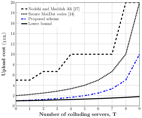
Compared to [27], which also considers the general case with the source nodes separate from the user, our scheme provides significant improvements in terms of the upload cost. The upload cost achieved by the scheme in [27] is given by $\chi_{UL}=\frac{\min(2K^{2}+2T-3,K^{2}+KT+T-2)}{K}$, which is significantly higher than that provided by our scheme (see Fig. 2). We also highlight that, as opposed to the scheme in [27], our scheme does not require inter-server communication in the computation and communication phases for multiplying two matrices, which significantly reduces both the latency and the complexity.

References

- [1] S. Rane, W. Sun, and A. Vetro, “Secure function evaluation based on secret sharing and homomorphic encryption,” in Annual Allerton Conf. on Comm., Control, and Computing, Sep. 2009, pp. 827–834.
- [2] M. Yasuda, T. Shimoyama, J. Kogure, K. Yokoyama, and T. Koshiba, “Secure statistical analysis using rlwe-based homomorphic encryption,” in Information Security and Privacy, E. Foo and D. Stebila, Eds. Cham: Springer International Publishing, 2015, pp. 471–487.
- [3] D. H. Duong, P. K. Mishra, and M. Yasuda, “Efficient secure matrix multiplication over lwe-based homomorphic encryption,” Tatra Mountains Mathematical Publications, vol. 67, no. 1, pp. 69 – 83, 2016. [Online]. Available: https://content.sciendo.com/view/journals/tmmp/67/1/article-p69.xml
- [4] M. Yasuda, T. Shimoyama, J. Kogure, K. Yokoyama, and T. Koshiba, “Practical packing method in somewhat homomorphic encryption,” in Data Privacy Management and Autonomous Spontaneous Security. Berlin, Heidelberg: Springer Berlin Heidelberg, 2014, pp. 34–50.
- [5] N. J. Bouman and N. de Vreede, “New protocols for secure linear algebra: Pivoting-free elimination and fast block-recursive matrix decomposition,” IACR Cryptology ePrint Archive, vol. 2018, p. 703, 2018.
- [6] R. Cramer and I. Damgård, “Secure distributed linear algebra in a constant number of rounds,” in Advances in Cryptology — CRYPTO 2001, J. Kilian, Ed. Berlin, Heidelberg: Springer Berlin Heidelberg, 2001, pp. 119–136.
- [7] K. Lee, M. Lam, R. Pedarsani, D. Papailiopoulos, and K. Ramchandran, “Speeding up distributed machine learning using codes,” IEEE Transactions on Information Theory, vol. 64, no. 3, pp. 1514–1529, March 2018.
- [8] R. Tandon, Q. Lei, A. G. Dimakis, and N. Karampatziakis, “Gradient coding: Avoiding stragglers in distributed learning,” in Proceedings of the 34th International Conference on Machine Learning, ser. Proceedings of Machine Learning Research, D. Precup and Y. W. Teh, Eds., vol. 70. International Convention Centre, Sydney, Australia: PMLR, 06–11 Aug 2017, pp. 3368–3376. [Online]. Available: http://proceedings.mlr.press/v70/tandon17a.html
- [9] Q. Yu, M. Maddah-Ali, and S. Avestimehr, “Polynomial codes: an optimal design for high-dimensional coded matrix multiplication,” in Advances in Neural Information Processing Systems 30, I. Guyon, U. V. Luxburg, S. Bengio, H. Wallach, R. Fergus, S. Vishwanathan, and R. Garnett, Eds. Curran Associates, Inc., 2017, pp. 4403–4413. [Online]. Available: http://papers.nips.cc/paper/7027-polynomial-codes-an-optimal-design-for-high-dimensional-coded-matrix-multiplication.pdf
- [10] S. Dutta, M. Fahim, F. Haddadpour, H. Jeong, V. Cadambe, and P. Grover, “On the optimal recovery threshold of coded matrix multiplication,” IEEE Transactions on Information Theory, vol. 66, no. 1, pp. 278–301, Jan 2020.
- [11] S. Dutta, Z. Bai, H. Jeong, T. M. Low, and P. Grover, “A unified coded deep neural network training strategy based on generalized polydot codes,” 2018 IEEE International Symposium on Information Theory (ISIT), pp. 1585–1589, 2018.
- [12] Q. Yu, M. A. Maddah-Ali, and A. S. Avestimehr, “Straggler mitigation in distributed matrix multiplication: Fundamental limits and optimal coding,” in 2018 IEEE International Symposium on Information Theory (ISIT), June 2018, pp. 2022–2026.
- [13] Q. Yu, N. Raviv, J. So, and A. S. Avestimehr, “Lagrange coded computing: Optimal design for resiliency, security and privacy,” CoRR, vol. abs/1806.00939, 2018. [Online]. Available: http://arxiv.org/abs/1806.00939
- [14] I. S. Reed and G. Solomon, “Polynomial codes over certain finite fields,” Journal of the Society for Industrial and Applied Mathematics, vol. 8, no. 2, pp. 300–304, 1960. [Online]. Available: https://doi.org/10.1137/0108018
- [15] B. Hasircioglu, J. Gómez-Vilardebó, and D. Gündüz, “Bivariate polynomial coding for exploiting stragglers in heterogeneous coded computing systems,” ArXiv, vol. abs/2001.07227, 2020.
- [16] W.-T. Chang and R. Tandon, “On the capacity of secure distributed matrix multiplication,” arXiv e-prints, Jun. 2018.
- [17] A. Shamir, “How to share a secret,” Commun. ACM, vol. 22, no. 11, pp. 612–613, Nov. 1979. [Online]. Available: http://doi.acm.org/10.1145/359168.359176
- [18] R. D’Oliveira, S. El Rouayheb, and D. Karpuk, “GASP codes for secure distributed matrix multiplication,” arXiv e-prints, Dec. 2018.
- [19] Z. Jia and S. A. Jafar, “On the Capacity of Secure Distributed Matrix Multiplication,” arXiv e-prints, Aug. 2019.
- [20] K. Banawan and S. Ulukus, “Multi-message private information retrieval: Capacity results and near-optimal schemes,” IEEE Transactions on Information Theory, vol. 64, no. 10, pp. 6842–6862, Oct 2018.
- [21] R. Tajeddine, O. W. Gnilke, D. Karpuk, R. Freij-Hollanti, and C. Hollanti, “Private information retrieval from coded storage systems with colluding, Byzantine, and unresponsive servers,” IEEE Transactions on Information Theory, vol. 65, no. 6, pp. 3898–3906, June 2019.
- [22] Q. Yu and A. S. Avestimehr, “Entangled polynomial codes for secure, private, and batch distributed matrix multiplication: Breaking the "cubic" barrier,” CoRR, vol. abs/2001.05101, 2020. [Online]. Available: https://arxiv.org/abs/2001.05101
- [23] Z. Chen, Z. Jia, Z. Wang, and S. A. Jafar, “GCSA codes with noise alignment for secure coded multi-party batch matrix multiplication,” in 2020 IEEE International Symposium on Information Theory (ISIT). IEEE, jun 2020. [Online]. Available: https://doi.org/10.1109%2Fisit44484.2020.9174230
- [24] M. Aliasgari, O. Simeone, and J. Kliewer, “Distributed and private coded matrix computation with flexible communication load,” in 2019 IEEE International Symposium on Information Theory (ISIT), July 2019, pp. 1092–1096.
- [25] S. Dutta, M. Fahim, F. Haddadpour, H. Jeong, V. Cadambe, and P. Grover, “On the optimal recovery threshold of coded matrix multiplication,” arXiv e-prints, Jan. 2018.
- [26] J. Kakar, A. Khristoforov, S. Ebadifar, and A. Sezgin, “Uplink-downlink tradeoff in secure distributed matrix multiplication,” ArXiv, vol. abs/1910.13849, 2019.
- [27] H. A. Nodehi and M. A. Maddah-Ali, “Limited-sharing multi-party computation for massive matrix operations,” in 2018 IEEE International Symposium on Information Theory (ISIT), June 2018, pp. 1231–1235.
- [28] M. Ben-Or, S. Goldwasser, and A. Wigderson, Completeness Theorems for Non-Cryptographic Fault-Tolerant Distributed Computation. New York, NY, USA: Association for Computing Machinery, 2019, p. 351–371. [Online]. Available: https://doi.org/10.1145/3335741.3335756
- [29] S. Lin, T. Y. Al-Naffouri, Y. S. Han, and W. Chung, “Novel polynomial basis with fast Fourier transform and its application to Reed-Solomon erasure codes,” IEEE Transactions on Information Theory, vol. 62, no. 11, pp. 6284–6299, 2016.
- [30] J. Kakar, S. Ebadifar, and A. Sezgin, “Rate-efficiency and straggler-robustness through partition in distributed two-sided secure matrix computation,” ArXiv, vol. abs/1810.13006, 2018.
- [31] A. Borodin and R. Moenck, “Fast modular transforms,” Journal of Computer and System Sciences, vol. 8, no. 3, pp. 366 – 386, 1974. [Online]. Available: http://www.sciencedirect.com/science/article/pii/S0022000074800292
- [32] M. Ylinen, A. Burian, and J. Takala, “Direct versus iterative methods for fixed-point implementation of matrix inversion,” in IEEE Int’l Symposium on Circuits and Systems, vol. 3, 2004, pp. III–225.