Density-Fixing: Simple yet Effective Regularization Method
based on the Class Priors
Abstract
Machine learning models suffer from overfitting, which is caused by a lack of labeled data. To tackle this problem, we proposed a framework of regularization methods, called density-fixing, that can be used commonly for supervised and semi-supervised learning. Our proposed regularization method improves the generalization performance by forcing the model to approximate the class’s prior distribution or the frequency of occurrence. This regularization term is naturally derived from the formula of maximum likelihood estimation and is theoretically justified. We further provide the several theoretical analyses of the proposed method including asymptotic behavior. Our experimental results on multiple benchmark datasets are sufficient to support our argument, and we suggest that this simple and effective regularization method is useful in real-world machine learning problems.
1 Introduction
Machine learning has achieved great success in many areas. However, such machine learning models suffer from an over-fitting problem caused by a lack of data [9, 19, 5]. To tackle such problems, research on semi-supervised learning [32, 15] or regularization [30, 27] has been very active.
We focus on leveraging the class density of the entire dataset as prior knowledge about labeled and unlabeled data. This means that we assume that the density of each class is obtained as prior knowledge. This assumption is a natural one in many actual machine learning problems. Based on this idea, we propose a framework of regularization methods, called density-fixing, both supervised and semi-supervised settings can commonly use that. Our proposed density-fixing regularization improves the generalization performance by forcing the model to approximate the class’s prior distribution or the frequency of occurrence. This regularization term of density-fixing is naturally derived from the formula for maximum likelihood estimation and is theoretically justified. We further investigated the asymptotic behavior of the density-fixing and how the regularization terms behave when assuming a prior distribution of several classes in practice. Our experimental results on multiple benchmark datasets are sufficient to support our argument, and we suggest that this simple and effective regularization method is useful in real-world problems.
Contribution: We propose the density-fixing regularization, which has the following properties:
- •
simplicity: density-fixing is very simple to implement and has almost no computational overhead.
- •
naturalness: density-fixing is derived naturally from the formula for maximum likelihood estimation and has a theoretical guarantee. We also provide several theoretical analyses.
- •
versatility: density-fixing is generally applicable to many problem settings.
In a nutshell, density-fixing forcing the balance of class density:
| (1) |
where is the some loss function (e.g. cross-entropy loss), and is the parameter of the regularization term. For the true distribution of a class, we can use it if it is given as prior knowledge, otherwise we can average the frequency of occurrence of the labels in the training sample and use it as an estimator :
| (2) |
The sample mean provides the unbiased and consistent estimator of the frequency of class occurrence, so it is sufficient to use it.
The source-code necessary to replicate our CIFAR-10 experiments is available at GitHub 11 1 https://github.com/nocotan/density_fixing.
2 Related Works
In this section, we introduce some related works that are relevant to our work.
2.1 Over-fitting and Regularization
Machine learning models suffer from an over-fitting problem caused by a lack of data. In order to avoid over-fitting, various regularization methods have been proposed. For example, Dropout [27] is a powerful regularization method that introduces ensemble learning-like behavior by randomly removing connections between neurons of the Deep Neural Network. Another recently proposed simple regularization method is mixup and its variants [30, 13, 29], which takes a linear combination of training data as a new input. There are many regularization methods for some specific models (e.g., for Generative Adversarial Networks [26, 14]).
2.2 Semi-Supervised Learning
There are many studies on semi-supervised learning [32, 33]. The method of assigning pseudo-labels to unlabeled data as new training data is very popular [20]. Another approach to semi-supervised learning is the use of Generative Adversarial Networks, which are famous for their expressive power [18].
3 Notations and Problem Formulation
Let be the input space, be the output space, be the number of classes and be a set of concepts we may wish to learn. We assume that each input vector is of dimension d. We also assume that examples are independently and identically distributed (i.i.d) according to some fixed but unknown distribution .
Then, the learning problem formulated as follows: we consider a fixed set of possible concepts , called hypothesis set. We receives a sample drawn i.i.d. according to as well as the labels , which are based on a specific target concept . In the semi-supervised learning problem, we additionally have access to unlabeled sample drawn i.i.d according to . Our task is to use the labeled sample and unlabeled sample to find a hypothesis that has a small generalization error for the concept . The generalization error is defined as follows.
Definition 1.
(Generalization error) Given a hypothesis , a target concept , and unknown distribution , the generalization error of is defined by
| (3) |
where is the indicator function of the event .
The generalization error of a hypothesis is not directly accessible since both the underlying distribution and the target concept are unknown Then, we have to measure the empirical error of hypothesis on the observable labeled sample . The empirical error is defined as follows.
Definition 2.
(Empirical error) Given a hypothesis , a target concept , and a sample , the empirical error of is defined by
| (4) |
In learning problems, we are interested in how much difference there is between empirical and generalization errors. Therefore, in general, we consider the relative generalization error . In the following sections, we derive a regularization method that reduces the relative generalization error and asymptotic behavior of our proposed method.
4 Density-Fixing Regularization
In this paper, we assume that is a class of functions mapping input vectors to the class densities:
| (5) |
Therefore, we can replace the learning problem with a problem that approximates the true distribution with the estimated distribution .
We assume that the class-conditional probability for labeled data and that for unlabeled data (or test data) are the same:
| (6) |
Then, our goal is to estimate from labeld data drawn i.i.d from and unlabeled data
Theorem 1.
Let be the estimated distribution parameterized by , and be the true distribution. Then, we can write the sum of log-likelihood function as follows:
| (7) |
where is the Kullback-Leibler divergence [17] from to :
| (8) | |||||
| (9) |
This means that when we consider maximum likelihood estimation, we can decompose the objective function into two terms: the term depending on and the term depending only on .
Proof.
From Bayes’ theorem, we can obtain
| (10) | |||||
| (11) |
Then, combining Eq (6), (10) and (11),
| (12) | |||||
The maximum likelihood estimator is the maximizer of the likelihood:
| (13) | |||||
Considering the maximization of the likelihood function, we can have the log-likelihood function as follows:
| (14) | |||||
Finally, we compute sum of log-likelihood function,
and then, we have Eq (7). ∎
Considering that we maximize Eq (7), it is clear that should be small value or closer to . The Kullback–Leibler divergence is defined if and only if , implies , and this property is so called absolute continuity.
From the above theorem, if the probability of class occurrence is known in advance, it can be used to perform regularization. We call this term density-fixing regularization. Regularization is performed so that the density of each class in the inference result for the unlabeled sample approximates the .
In addition, the well-known properties of KL-divergence also naturally lead to the following proposition about density-fixing.
Corollary 1.
(Zero-forcing property) The estimation that approximates satisfies .
Proof.
If we approximate and by continuous functions, then the KL-divergence is given as follows:
Since and are continuous functions and then, if at some point , there exists a neighborhood around , where . Therefore, if , will be very large in that neighborhood, which makes the integral grow very large. Thus, any minimization algorithm will result in a , where if . ∎
This mean that the best approximation satisfies
| (16) |
for at which . This property is called zero-forcing, and we can see that our regularization behave as if the probabilities of classes we do not know remain .

5 Asymptotic Normality
In this section, we discuss how the density-fixing regularization behaves asymptotically. In general, the bias of the estimator is defined by
| (17) |
when is the true parameter. An estimator is unbiased when .
The asymptotic theory studies the behavior of an estimator when sample size is large. When the bias satisfies
| (18) |
this estimator is asymptotically unbiased. It is known that the maximum likelihood estimator is asymptotically unbiased. This means that the maximum likelihood estimator converges to the true parameter as tends to infinity:
| (19) |
Then, the accuracy of an estimator is measured by the error covariance matrix, ,
| (20) |
The following theorem states that density-fixing reduces the error covariance of the maximum likelihood estimator depending on the shape of the distribution.
Theorem 2.
Let . The asymptotic variance of the maximum likelihood estimator applying the density-fixing regularization is given by . Here, is a function that always takes a positive value, parameterized by .
Proof.
In the maximum likelihood estimator for the number of samples , we can obtain the following by Taylor expansion of around :
here, we assume that has the third-order derivative with respect to parameter and be bounded. From Eq (5) and central limit theorem, we can obtain
| (22) |
when is sufficiently large. Here, is the Fisher information matrix:
| (23) |
Then, let as the original likelihood function, we can obtain
| (24) | |||||
Therefore, the maximum likelihood estimator applying the density-fixing regularization satisfies the following:
| (25) |
Here, let be the exponential family. An exponential family of probability distribution is written as
| (26) |
where is the natural parameter and is the sufficient statistcs of . Let and , we can have
| (27) | ||||
Here, expressing by through variable transformation, we obtain the following equation:
Then, the second-order derivative of is
| (30) |
This means that the second-order derivative of the log-likelihood function of the exponential family has always negative value. Therefore, we can obtain the proof of Theorem 2 with . ∎
This theorem implies that the convergence rate of the asymptotic variance of the maximum likelihood estimator becomes faster by by applying the density-fixing regularization. Figure 1 illustrates the asymptotic behavior of the estimator by our regularization.
5.1 Some Examples
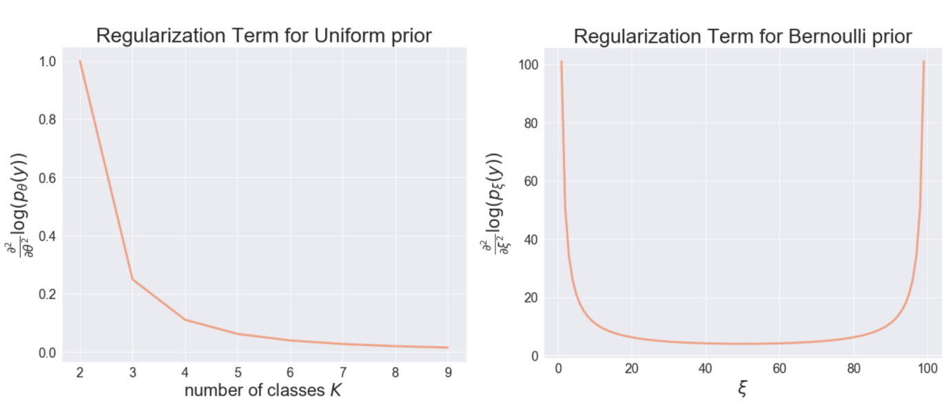
In this subsection, we investigate the behavior of our proposed method by assuming some class distributions as examples. To summarize our results:
- •
For discrete uniform distribution, the effect of regularization becomes weaker as the number of classes increases,
- •
For Bernoulli distribution, our regularization behaves to give strong regularization when there is a class imbalance.
Figure 2 shows the behavior of the regularization terms under each distribution.
5.1.1 Discrete Uniform Distribution
We assume that the probability density function of classes is as follows:
| (31) |
here is the number of classes. This is the discrete uniform distribution . From theorem 2, the following corollary can be derived.
Corollary 2.
The effect of regularization becomes weaker as the number of classes increase when the class probability follows a discrete uniform distribution.
Proof.
From theorem 2, the asymptotic behavior of density-fixing training is
| (32) |
It is clear that from the above equation. ∎
The discrete uniform distribution corresponds to the case of multi-class classification where all classes have the same probability of occurrence and is a general problem setup.

5.1.2 Bernoulli Distribution
We assume that and the probability density function of classes is as follows:
| (33) |
here and this is the Bernoulli distribution. This case is a binary classification problem.
Corollary 3.
For binary classification problem, our proposed method behaves to give strong regularization when there is a class imbalance.
Proof.
Our regularization term is
| (34) | |||||
and we can obtain the asymptotic behavior of density-fixing training as follows:
| (35) |
Thus, we can see that regularization is stronger when is away from . ∎
6 Connection to Knowledge Distillation
Knowledge distillation [11] is the model compression method in which a small model is trained to mimic a pre-trained larger model. The large pretrained model is called the teacher model and the small model learned by knowledge distillation is called the student model. In knowledge distillation, knowledge is transferred from the teacher model to the student model by minimizing a loss function in which the target is the distribution of class probabilities predicted by the teacher model. Furthermore, it has been shown that knowledge distillation can be used not only for model compression, but also for model regularization [7, 28]. For example, it has been experimentally shown that an iterative knowledge distillation method using the same architecture for teacher and student models contributes to the generalization performance of the models [7].
Let the output of the teacher model be and the output of the student model be . Here, the knowledge distillation scheme is formulated as follows:
| (36) |
where is the parameter. Comparing Eq (1) and Eq (36), we can see that the knowledge distillation loss function is a special case of the density-fixing loss function. In other words, knowledge distillation is the injection of knowledge extracted by the teacher model instead of human prior knowledge in density-fixing regularization. Thus, we can switch between density-fixing and knowledge distillation based on how much we know about the distribution of the data. Our proposed density-fixing is useful if we are very familiar with the distribution of the data, while knowledge distillation is useful if we have no knowledge of the data at all.
7 Experimental Results
In this section, we introduce our experimental results. We implement the density-fixing regularization as follows:
| (37) |
where is the cross-entropy loss and is the weight parameter for the regularization term. The implementation of density-fixing regularization is straightforward, Figure 7 shows the few lines of code necessary to implement density-fixing regularization in PyTorch [25].
The datasets we use are CIFAR-10 [16], CIFAR-100 [16], STL-10 [4] and SVHN [24]. We determined the prior distribution of classes based on the number of data accounted for in each class of the data set, and we used ResNet-18 [10] as the baseline model.
| Dataset | Model | Top 1 Error | Top 5 Error |
|---|---|---|---|
| CIFAR-10 | ResNet-18 | 12.720% | 0.812% |
| ResNet-18 + density-fixing () | 12.230% | 0.779% | |
| ResNet-18 + density-fixing () | |||
| ResNet-18 + density-fixing () | 12.341% | 0.770% | |
| CIFAR-100 | ResNet-18 | 25.562% | 6.710% |
| ResNet-18 + density-fixing () | 25.241% | 6.302% | |
| ResNet-18 + density-fixing () | 25.965% | 6.887% | |
| ResNet-18 + density-fixing () |
| dataset | ||||||
|---|---|---|---|---|---|---|
| CIFAR-10 | 28.235 | 28.510 | 29.086 | 30.964 | 30.892 | |
| CIFAR-100 | 66.622 | 66.723 | 66.861 | 66.895 | 67.007 | |
| STL-10 | 59.770 | 60.110 | 60.124 | 60.405 | 60.897 | |
| SVHN | 27.937 | 28.028 | 30.110 | 32.025 | 32.879 |

| Model | mean IOU |
|---|---|
| FCN ResNet-50 | |
| FCN ResNet-50 + density-fixing () | |
| FCN ResNet-50 + density-fixing () | |
| FCN ResNet-50 + density-fixing () | |
| FCN ResNet-50 + density-fixing () |
7.1 Supervised Classification
In this subsection, we introduce the supervised classification results, and we assumed a discrete uniform distribution for the class distribution.
Figure 3 shows the experimental results for CIFAR-10 with density-fixing regularization. As seen in the left of this figure, baseline model and density-fixing converge at a similar speed to their best test errors. At around epoch, a second loss reduction, Deep Double Descent [23], can be observed, but this phenomenon is not disturbed by density-fixing. From the right, we can see that by increasing the parameter , we can reduce the generalization gap.
Also, Table 1 shows the contribution of density-fixing to the reduction of test errors.
7.2 Semi-Supervised Classification
In this subsection, we introduce the semi-supervised classification results. In our experiments, we assumed a discrete uniform distribution for the class distribution and treated of the training data as labeled and of the training data as unlabeled.
Figure 4 show test loss and train-test differences for each in the semi-supervised setting. We can see that by increasing the parameter , it reduce the generalization gap. In addition, CIFAR-10 and CIFAR-100, which consist of images from the same domain, have and classes, respectively, but the experimental results show that CIFAR-10 has a more significant regularization effect than CIFAR-100. This result supports our example in Eq (32).
Table 2 shows a comparison of classification error for each . These experimental results show that our regularization leads to improving error on the test data.

7.3 Semantic Segmentation for the Pascal VOC Dataset
We present the results of an experiment on semantic segmentation in the Pascal VOC2012 dataset [6]. This dataset contains around labeled images belonging to categories.
We computed pixel-wise the frequency of class occurrence in the training data as a prior distribution to apply our density-fixing. We also used FCN ResNet50 [21] as a baseline model to investigate the performance difference with and without density-fixing.
Table 3 shows a comparison of mean IOU for each models. We can see that our density-fixing regularization can improve the performance.
Figure 5 shows the visualization of the semantic segmentation result. In this experiment, we apply our density-fixing with parameter . Recall that our density-fixing regularization has the zero-forcing property, and we can see that our regularization term contributes to eliminating the labels that never happens (e.g., the light green label in the first row which occurs in the result of FCN represents the sofa, and density-fixing eliminate it.).
7.4 Stabilization of Generative Adversarial Networks
Generative Adversarial Networks (GANs) [8] is one of the powerful generative model paradigms that are currently successful in various tasks, such as image generation [12, 2] and image-to-image translation [3, 31]. However, GANs have the problem that their learning is very unstable. To tackle this problem, many approaches have been proposed [22, 1]. We suggest that regularization by density-fixing contributes to improving the stability of GANs. The density-fixing formulation of GANs is:
| (38) |
where is the discriminator, is the generator, is the binary cross entropy and .
Figure 6 illustrates the stabilizing effect of density-fixing the training of GANs when modeling a toy dataset (blue samples). The neural networks in these experiments are fully-connected and have three hidden layers of ReLU units. We can see that density-fixing contributes to the stabilization of the training of GANs.

8 Conclusion and Discussion
In this paper, we proposed a framework of regularization methods that can be used commonly for both supervised and semi-supervised learning. Our proposed regularization method improves the generalization performance by forcing the model to approximate the prior distribution of the class. We proved that this regularization term is naturally derived from the formula of maximum likelihood estimation. We further investigated the asymptotic behavior of the proposed method and how the regularization terms behave when assuming a prior distribution of several classes in practice. Our experimental results have sufficiently demonstrated the effectiveness of our proposed method.
References
- [1] Martin Arjovsky, Soumith Chintala, and Léon Bottou. Wasserstein generative adversarial networks. In International Conference on Machine Learning, pages 214–223, 2017.
- [2] Andrew Brock, Jeff Donahue, and Karen Simonyan. Large scale gan training for high fidelity natural image synthesis. In International Conference on Learning Representations, 2018.
- [3] Yunjey Choi, Minje Choi, Munyoung Kim, Jung-Woo Ha, Sunghun Kim, and Jaegul Choo. Stargan: Unified generative adversarial networks for multi-domain image-to-image translation. In Proceedings of the IEEE conference on computer vision and pattern recognition, pages 8789–8797, 2018.
- [4] Adam Coates, Andrew Ng, and Honglak Lee. An analysis of single-layer networks in unsupervised feature learning. In Proceedings of the fourteenth international conference on artificial intelligence and statistics, pages 215–223, 2011.
- [5] Tom Dietterich. Overfitting and undercomputing in machine learning. ACM computing surveys (CSUR), 27(3):326–327, 1995.
- [6] M. Everingham, S. M. A. Eslami, L. Van Gool, C. K. I. Williams, J. Winn, and A. Zisserman. The pascal visual object classes challenge: A retrospective. International Journal of Computer Vision, 111(1):98–136, Jan. 2015.
- [7] Tommaso Furlanello, Zachary Lipton, Michael Tschannen, Laurent Itti, and Anima Anandkumar. Born again neural networks. In International Conference on Machine Learning, pages 1607–1616, 2018.
- [8] Ian Goodfellow, Jean Pouget-Abadie, Mehdi Mirza, Bing Xu, David Warde-Farley, Sherjil Ozair, Aaron Courville, and Yoshua Bengio. Generative adversarial nets. In Advances in neural information processing systems, pages 2672–2680, 2014.
- [9] Douglas M Hawkins. The problem of overfitting. Journal of chemical information and computer sciences, 44(1):1–12, 2004.
- [10] Kaiming He, Xiangyu Zhang, Shaoqing Ren, and Jian Sun. Deep residual learning for image recognition. In Proceedings of the IEEE conference on computer vision and pattern recognition, pages 770–778, 2016.
- [11] Geoffrey Hinton, Oriol Vinyals, and Jeffrey Dean. Distilling the knowledge in a neural network. In NIPS Deep Learning and Representation Learning Workshop, 2015.
- [12] Tero Karras, Timo Aila, Samuli Laine, and Jaakko Lehtinen. Progressive growing of gans for improved quality, stability, and variation. In International Conference on Learning Representations, 2018.
- [13] Masanari Kimura. Mixup training as the complexity reduction. arXiv preprint arXiv:2006.06231, 2020.
- [14] Masanari Kimura and Takashi Yanagihara. Anomaly detection using gans for visual inspection in noisy training data. In Asian Conference on Computer Vision, pages 373–385. Springer, 2018.
- [15] Durk P Kingma, Shakir Mohamed, Danilo Jimenez Rezende, and Max Welling. Semi-supervised learning with deep generative models. In Advances in neural information processing systems, pages 3581–3589, 2014.
- [16] Alex Krizhevsky, Geoffrey Hinton, et al. Learning multiple layers of features from tiny images. 2009.
- [17] S. Kullback and R. A. Leibler. On information and sufficiency. Ann. Math. Statist., pages 22:79–86, 1951.
- [18] Abhishek Kumar, Prasanna Sattigeri, and Tom Fletcher. Semi-supervised learning with gans: Manifold invariance with improved inference. In Advances in Neural Information Processing Systems, pages 5534–5544, 2017.
- [19] Steve Lawrence, C Lee Giles, and Ah Chung Tsoi. Lessons in neural network training: Overfitting may be harder than expected. In AAAI/IAAI, pages 540–545. Citeseer, 1997.
- [20] Dong-Hyun Lee. Pseudo-label: The simple and efficient semi-supervised learning method for deep neural networks. In Workshop on challenges in representation learning, ICML, volume 3, 2013.
- [21] Jonathan Long, Evan Shelhamer, and Trevor Darrell. Fully convolutional networks for semantic segmentation. In Proceedings of the IEEE conference on computer vision and pattern recognition, pages 3431–3440, 2015.
- [22] Takeru Miyato, Toshiki Kataoka, Masanori Koyama, and Yuichi Yoshida. Spectral normalization for generative adversarial networks. In International Conference on Learning Representations, 2018.
- [23] Preetum Nakkiran, Gal Kaplun, Yamini Bansal, Tristan Yang, Boaz Barak, and Ilya Sutskever. Deep double descent: Where bigger models and more data hurt. In International Conference on Learning Representations, 2020.
- [24] Yuval Netzer, Tao Wang, Adam Coates, Alessandro Bissacco, Bo Wu, and Andrew Y Ng. Reading digits in natural images with unsupervised feature learning. 2011.
- [25] Adam Paszke, Sam Gross, Francisco Massa, Adam Lerer, James Bradbury, Gregory Chanan, Trevor Killeen, Zeming Lin, Natalia Gimelshein, Luca Antiga, et al. Pytorch: An imperative style, high-performance deep learning library. In Advances in neural information processing systems, pages 8026–8037, 2019.
- [26] Kevin Roth, Aurelien Lucchi, Sebastian Nowozin, and Thomas Hofmann. Stabilizing training of generative adversarial networks through regularization. In Advances in neural information processing systems, pages 2018–2028, 2017.
- [27] Nitish Srivastava, Geoffrey Hinton, Alex Krizhevsky, Ilya Sutskever, and Ruslan Salakhutdinov. Dropout: a simple way to prevent neural networks from overfitting. The journal of machine learning research, 15(1):1929–1958, 2014.
- [28] Qizhe Xie, Minh-Thang Luong, Eduard Hovy, and Quoc V Le. Self-training with noisy student improves imagenet classification. In Proceedings of the IEEE/CVF Conference on Computer Vision and Pattern Recognition, pages 10687–10698, 2020.
- [29] Sangdoo Yun, Dongyoon Han, Seong Joon Oh, Sanghyuk Chun, Junsuk Choe, and Youngjoon Yoo. Cutmix: Regularization strategy to train strong classifiers with localizable features. In Proceedings of the IEEE International Conference on Computer Vision, pages 6023–6032, 2019.
- [30] Hongyi Zhang, Moustapha Cisse, Yann N. Dauphin, and David Lopez-Paz. mixup: Beyond empirical risk minimization. In International Conference on Learning Representations, 2018.
- [31] Jun-Yan Zhu, Taesung Park, Phillip Isola, and Alexei A Efros. Unpaired image-to-image translation using cycle-consistent adversarial networks. In Proceedings of the IEEE international conference on computer vision, pages 2223–2232, 2017.
- [32] Xiaojin Zhu and Andrew B Goldberg. Introduction to semi-supervised learning. Synthesis lectures on artificial intelligence and machine learning, 3(1):1–130, 2009.
- [33] Xiaojin Jerry Zhu. Semi-supervised learning literature survey. Technical report, University of Wisconsin-Madison Department of Computer Sciences, 2005.