Giant micropulse emission in the Vela pulsar at C bandJournal: ApJ
Abstract
We present here the analysis of giant micropulses from the Vela pulsar. A total of 4187 giant micropulses with peak flux density 2.5 Jy were detected during almost 4 hours of observations carried out with the Yunnan 40-m radio telescope at 6800 MHz. Nine of the giant micropulses arrived approximately 3 to 4 ms earlier than the peak of average pulse profile, longer than that at lower frequencies. The remaining giant micropulses were clustered into three distributions which correspond to three main emission regions, including four occurring on the trailing edge of averaged profile. We find that the peak flux density distribution follows a power law with index . Furthermore, a certain amount of memory is present from the giant micropulse waiting time distribution. Possible emission mechanisms are discussed.
Keywords:
pulsars: general – pulsars: individual (Vela) – radiation mechanisms:non-thermalI Introduction
Vela pulsar (PSR J08354510 or B083345) is a multi-wavelength emitting, young, close, luminous and isolated neutron star associated with the Vela supernova remnant in the constellation of Vela. It is known to emit giant micropulses with high peak flux density and narrow pulse width, which are located at the leading edge of the pulse profile both at 660 MHz and 1413 MHz (Johnston et al. 2001). No genuine giant pulses have been detected since their mean flux densities do not exceed 10 times the mean flux density of average pulse profile, according to the working giant pulse definition (Knight 2006). The giant micropulses at 2.3 GHz were observed to have a power-law distribution of flux density with a slope of (Kramer et al. 2002). Consecutive bright radio pulses with five times the flux of the average pulse were detected at 1440 MHz, which suggests that the individual bright pulses may not be independent random events (Palfreyman et al. 2011).
At lower observing frequencies, the pulse scatter broadening smooths over the microstructure features, and the pulse intensity fluctuates in time and frequency domains caused by the interstellar scintillation. These effects can be ruled out at higher frequencies. Nonetheless, no giant micropulses above 2.3 GHz have been mentioned in the literatue. Furthermore, whether giant micropulses are limited in the leading edge of the average pulse profile, and whether they evolve with observing frequencies, are necessary to be investigated. No strict naming convention for giant micropulses has been formalized. In this paper, we present results of giant micropulse emission (peak flux density 2.5 Jy) from the Vela pulsar at higher frequency. The nomenclature of giant micropulse will be used here for continuty. In Section II, we describe our observations and data reduction. We show the results on giant micropulse emission in Section III. In Section IV, we discuss our findings.
II Observations and Data Reduction
The Vela pulsar was observed on 17 August, 2019 using the Yunnan 40-m radio telescope in a frequency band centered at 6800 MHz. The orthogonal linear polarizations with a bandwidth of 800 MHz (508 MHz is usable) were injected into a cryogenic receiving system. Then the output power was recorded with 1024 channels over the passband using a ROACH211 1 https://casper.berkeley.edu/wiki/ROACH2 based digital filterbank system with an effective sampling time of 40.96 s.
Observations of individual pulses from the vela pulsar allowed us to perform a variety of analysis techniques which we describe below. Before performing the analysis, data were converted into the filterbank format required for the SIGPROC22 2 http://sigproc.sourceforge.net/ analysis package, and only the total intensity (Stokes I) was preserved. The radio frequency interference (RFI) was rejected by excluding narrow band as well as bursty broad band RFI by visual inspection. Incoherent de-dispersion was performed to remove sub-channel dispersive smearing using a dispersion measure (DM) of 67.97 pc cm-3(Petroff et al. 2013). Then, the data were folded to 2182 phase bins across the period with the ephemery of the pulsar, using the TEMPO33 3 http://tempo.sourceforge.net/ package to obtain a single pulse sequence for further analysis. In total, almost 4-hour successive observations we observed over 150,000 rotations of the pulsar.
Subsequently, the temporally resolved pulses were converted to flux based on a nominal system temperature of 40 K and efficiency of 50% for the C band receiver, since no flux calibrators were observed. With these values, the average flux density is measured to be mJy by integrating intesity of the folded pulse profile over the entire period. Generally, the pulsar spectra follow a simple power law , where is the mean flux density at the observing frequency and is the spectral index (Sieber 1973). However, the Vela pulsar presents a broken power-law spectral form with a spectral index of before and after a spectral break at MHz (Jankowski et al. 2018). According to the recent measure of the mean flux density ( mJy) at 5000 MHz (Zhao et al. 2019), the derived mean flux density from the power-law relationship at 6800 MHz is mJy, which is consistent with our measurement.
A pulse phase blind search algorithm was carried out to select giant micropulses in the whole de-dispersed timestreams, which are required to have signal-to-noise ratio (S/N) larger than 10. The detection threshold corresponds to a limiting flux of 2.5 Jy. This yielded a complete sample of 4187 giant micropulses were detected, most of which are close to the detection threshold.
III Results
Figure 1 shows where the giant micropulses arrive relative to the average pulse profile. Three main emission regions correspond to the leading, central and trailing components of the average pulse profile, and the phase boundaries are shown with vertical dashed lines. The giant micropulse emission are present at a wide phases, not just prior to the main pulse window as reported by Johnston et al. 2001. Three clusters are presented with four giant micropulses falling in the trailing edge of the pulse profile, which are consistent with three main emission regions. It is worthy to note that nine giant micropulses appear at the pulse phase prior to the nominal main emission window. The maximum phase jitter between giant micropulses and the main pulse peak is measured to be 4 ms, which is greater than that of 2.2 ms at 1413 MHz (Johnston et al. 2001). The brightest of these has a peak flux density in excess of 21.8 Jy, almost 40 times the peak flux density in the integrated pulse profile. Very little overall effect on the integrated profile is resulted from these giant micropulses. This may give an indication of the nature of the pulse emission process.

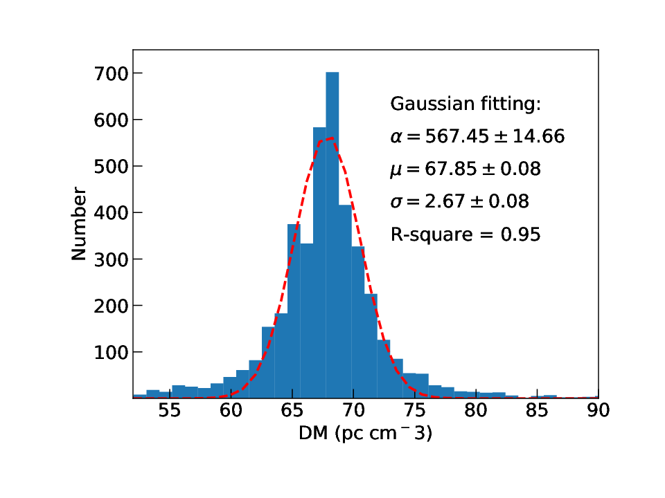
In order to identify whether the giant micropulses are originated from the Velar pulsar or terrestrial interference, the selected signals with S/N above the detection threshold are reprocessed with DM varying from 0 to 140 pc cm-3 in steps of 0.14 pc cm-3. To each DM, the time series after de-dispersion are shown in the lower left panels of Figure 2. The burst dissolves as the DM increases or decreases from the nominal DM of 67.97 pc cm-3, which provides a significant criterion for identifying a real burst. We are confident that the giant micropulses presented are not influenced by spurious signals after visual inspection, since no sources of interference are seen with dispersion like that of the Vela pulsar. Then the DM of a giant micropulse is calculated from the maximum amplitude over the whole pulse period (shown in the lower right panels). The middle left panels present four example dynamic spectra of the detected pulses. The dispersive sweep of the burst is clearly shown in the patchy spectra, which further demonstrates the authenticity of the pulses. Figure 3 shows the histogram for the DMs derived from all giant micropulses. The mean value of DM is 67.39 pc cm-3, which is in agreement with the value published by Petroff et al. 2013.


As reported by Johnston et al. 2001, a threshold of larger than 25 was taken to pick out the giant micropulses at 1413 MHz. The parameter is defined as , where is the maximum intensity, is the mean intensity and is the rms in the th bin. The phase-resolved at 6800 MHz is shown in Figure 4. Two peaks are clearly presented in the leading and leading edge of the pulse, which implies the existence of giant micropulses with extremely high amplitude with respect to the mean intensity in these phase ranges. And the value of decreases exponentially in the center and trailing of the pulse, which is inconsistent with the Gaussian statistics at 1413 MHz. As shown in Figure 1, the giant micropulse emission in the center component have higher occurrence rate and higher amplitude than that in the trailing component. Furthermore, none detection of giant micropulses with significant -value occur in the bump region.

The main panel of Figure 5 shows a scatter plot of peak flux density and the full width of half maximum (FWHM) for detected giant micropulses. The pulse broadening caused by inner-channel dispersion (1.4 s) and scattering (1.0 ns) is negelected due to high observing frequency. To obtain the FWHM, a Gaussian function is adopted to fit each giant micropulse. The position of the center of the peak is kept fixed with the pulse phase of the maximum value. Then FWHM is given by , where is the determined parameter using the least-square method. The giant micropulses have timescales (1.55 ms) much smaller than that of the average pulse profile (2.62 ms). As can be seen, the majority of giant micropulses tend to cluster in width of 50 to 500 s. In this interval, the width of a giant micropulse seems to be independent of its peak flux density, which is consistent with the result at 2.3 GHz (Kramer et al. 2002). The pulse-to-pulse energy distribution is served as one of the important differentiator between various emission processes (Burke-Spolaor et al. 2012). Probability density function (PDF) for the peak flux densities is shown in the upper panel, which is well described by a power law. The slope, obtained via least-square fitting, is give by , which is the steepest distribution to our best knowledge. While a logarithmic normal distribution is presented for the PDF formed from the peak flux densities of normal pulses, as shown in Figure 6. The distinctive distributions between giant micropulses and normal pulses may indicate their different emission mechanism. The pulse energies of the bursts from the Vela pulsar do not exceed 10 times the corresponding mean quantity. Nevertheless, the peak flux densities of the bursts are very large in absolute terms. For example, the brightest pulse detected corresponds to a peak flux density of approximately 28 Jy, which is 46 times the peak flux density of averaged profile. The pulse width PDF is given in the right panel, which clearly shows a normal distribution centered at around 250 s. In order to test if the pulse width PDF is multimodal for FWHMs, we model it as a sum of Gaussian distributions and a lognormal distribution. Models composed of one and up to three Gaussians and a lognormal distribution are tested against the data. The best fits obtained are presented in the right panel of Figure 5. Table 1 gives the parameters of the models using the maximum likelihood technique. The lognormal distribution gives the best description of the pulse width PDF using the Akaike information criterion (Akaike 1974, AIC,). We note, however, that distinctive distributions are presented for the phase resolved pulse width distributions as shown in Figure 7. The histograms of pulse widths for the first and third clusters both show normal distributions, where the third cluster has a greater typical width than the first cluster. While, a lognormal distribution is presented for the pulse width histogram for the second giant micropulse cluster. The best-fit values of the amplitude , the mean and the standard deviation of normal distributions for C1 and C3 and a lognormal distribution for C2 are listed in Table 2.
| Parameters | 1-G | 2-G | 3-G | Lognormal |
|---|---|---|---|---|
| 1 | 0.73 | 0.66 | 1 | |
| 0.23 | 0.22 | 0.23 | -1.30 | |
| 0.15 | 0.12 | 0.10 | 0.66 | |
| … | 0.27 | 0.04 | … | |
| … | 0.48 | 0.08 | … | |
| … | 0.28 | 0.02 | … | |
| … | … | 0.30 | … | |
| … | … | 0.46 | … | |
| … | … | 0.27 | … | |
| R-square | 0.93 | 0.96 | 0.98 | 0.95 |
| 888.49 | 198.64 | 208.80 | 168.88 | |
| 719.61 | 29.76 | 39.92 | 0 | |
| 1 |
Notes. The label -G in each column denotes the model of a sum of Gaussians. , and are the weight, mean and the standard deviation of the component of the sum of Gaussians. , and represent the AIC value, the relative respect to the model with the minimum value, and the Akaike weights of the model, respectively. R-square stands for the value of goodness of fit.


| Parameters | |||
|---|---|---|---|
| C1 | 1773 | 0.2380.002 | 0.1160.002 |
| C2 | 79.50.9 | -1.3360.002 | 0.4760.007 |
| C3 | 543 | 0.530.02 | 0.330.02 |
In order to investigate whether a giant micropulse is related to or independent of the previous one, the intervals between successive giant micropulses (waiting time, ) are calculated. The statistics of waiting time is intensively studied for solar flares, which can provide critical information about how an individual event occurs (Wheatland 2000). The waiting time PDF shown in Figure 8 presents a domination of short waiting times (25 periods), which indicates the production of giant micropulses occur in clusters, in other words, with a certain amount of memory. It leads us to interpret the distribution of giant micropulse waiting time with the Weibull distribution:
| (1) |
where is the reciprocal of the mean occurrence rate. Using the maximum-likelihood estimation, the best fitting coefficients are , , and R-square = 0.99. A implies that the probability of a giant micropulse occurring decreases with time, namely, the giant micropulse occurrence is clustered. A describes that the occurrence probability is zeros for consecutive giant micropulses. The estimated occurrence rate is higher than that calculated from our observation, which appears to be resulted from the clustering effect. A simple Poisson process, where the probability of a giant micropulse occurring is time invariant, produces an exponential distribution, which is fitted poorly as shown in the yellow dashed line. The best-fitted power-law distribution with an index of 0.02 does not fit the waiting time distributions well, as shown in Figure 8.

IV Discussion
The origin of giant pulses has been remaining a mystery since the discovery of giant pulses from Crab pulsar (Staelin & Reifenstein 1968). The generation of giant pulse activity was pointed to be an intrinsic phenomenon within the pulsar (Hankins 1971). The Giant pulses are supposed to be the product of induced Compton scattering of the radio radiation off the plasma in the pulsar magnetosphere (Petrova 2006). The extremely high intensity is as well caused by an enhanced number of charges partaking in the nonthermal, coherent radiation processes (Hankins et al. 2003). Alternatively, the origination of giant pulses is proposed from the coherent instability of plasma near the magnetic equator of light cylinder (Wang et al. 2019). Singal & Vats 2012 suggested that the giant pulse emission and nulling may be opposite manifestations of the same physical process. The giant pulses are suggested to occur in pulsars with extremely high magnetic fields at the light cylinder of G (Cognard et al. 1996). Therefore, the giant pulses are proposed to be originated near the light cylinder (Istomin 2004). However, the giant pulses are also detected in the pulsars with ordinary magnetic fields at the light cylinder of G, such as PSRs B003107 (Kuzmin & Ershov 2004), B1112+50 (Ershov & Kuzmin 2003), J1752+2359 (Ershov & Kuzmin 2005), B0950+08 (Smirnova 2012). B0656+14 (Kuzmin & Ershov 2006), B1237+25 (Kazantsev & Potapov 2017) and B0301+19 (Kazantsev et al. 2019), and it does not seem to support the high hypothesis. The Vela giant micropulse emission physics maybe independent on the high magnetic field at the light cylinder. Although the Vela’s is about 20 times smaller than that of PSR B1937+21 and the Crab pulsar, it is still in the top 5% of pulsars with estimate. The giant pulses from PSR J18242452A occur in narrow phase windows that correlate in phase with X-ray emission, and the two emission phenomena likely originate from the similar magnetospheric regions but not the same physical mechanism (Knight et al. 2006). In order to reveal the nature of the giant micropulses, simultaneous radio and X-ray observations on the Vela pulsar will be required.
Considering a scenario of narrow band emission, the high-frequency emission is assumed to be generated at low altitude and vice verse, called radio-to-frequency mapping (RFM) (Cordes 1978). This empirical relationship is well demonstrated from the Vela pulsar, the integrated pulse profile becomes narrower and narrower along with the increasing frequency (Liu et al. 2019). Plausible interpretations are proposed for the two types of giant micropulse emission. The giant micropulses may originate from two different emission regions in the pulsar magnetosphere. A certain amount of memory shown in the occurrance of giant micropulses may indicate that the normal giant micropulses are likely arised from the homologous region with the normal pulse emission, but with a different plasma state, since they are coincident with averaged profile in pulse phase. For instance, the fluctuations in the number of charges partaking in the coherent radiation process that gives rise the intense variation in the net radio emission of the pulse intensity, These kind of giant micropulses are emitted with high occurrance rate, because the frequent turbulence of plasma in the inner acceleration region could result in the enhancement of subbeam emission. While the leading giant micropulses are likely originated from a higher altitude within the same magnetic flux tube than the normal pulses. In this model, the giant micropulses are supposed to be accompanied by normal pulse emission, which are shown in some cases. However, according to the RFM, the higher frequency the narrower pulse width, which is inconsistent with the fact that our observed jitter in the arrival times at 6800 MHz is greater than that at lower frequencies. Therefore, the giant micropulses at different frequencies may be emitted from different magnetic field lines. The giant micropulse emission region at higher frequency is closer to the last open dipolar field lines than that at low frequency.
The Vela pulsar is known to be active in glitching, at least 7 glitches have been reported since 2003 44 4 http://www.atnf.csiro.au/research/pulsar/psrcat/. An intensive single-pulse observing campaign of the Vela pulsar at 1376 MHz showed that the pulse profile varied temporally, and was affected with a micro-glitch (Palfreyman et al. 2016). Furthermore, recent analysis of the 2016 glitch in the Vela pulsar, the accompanying alteration of the magnetospheric was observed (Palfreyman et al. 2018). Therefore, the detailed phase distribution of giant micropulses possibly provide additional clues on how the magnetosphere changes. As suggested by Palfreyman et al. 2016, the widening of emission cone could be caused by a glitch since the emission beam approaches the line of sight. Meanwhile, the giant micropulse distribution broadens under the assumption that both regular and giant micropulses originate from the same emission region. Futhermore, The glitch could lead to the increase of the plasma density in open field lines. The coherent instability enhances due to plasma oscillation. Then the giant micropulses within the emission window emerge, which broadens the distribution. The variation of pulse phase distribution of giant micropulses after the 2016 glitch is the topic of continuing observations. The radio spectrum of giant pulses shows a power-law distribution, its spectral index is compared to the average pulse value for a pulsar (Popov et al. 2006). The giant pulses do not occur simultaneously in both frequency ranges (Popov & Stappers 2003). Our detected giant micropulse rate at 6800 MHz is 1/36, which is higher than the previous bright pulse rate at 1376 MHz. The rate of bright pulse activity was reported to increase after some micro-glitches (Palfreyman et al. 2016). Therefore, this increase in statistics is possible to be affected by the glitches. The separation of giant pulse emission regions at lower frequency is larger than that at higher frequency for PSR B003107 (Kuzmin & Ershov 2004), which is contrary to the Vela pulsar. Therefore, the temporal evolution is preferrable to cause the observed difference in the pulse phase distribution of giant micropulses.
Further long-term simultaneous multi-frequency single pulse observations with full Stokes parameters would be very worthwhile in discerning the pulse emission mechanism and glitching process.
Acknowledgements
We thank the referee for comments which improved the paper. Much of this work was made possible by grant support from the West Light Foundation of Chinese Academy of Sciences (WLFC 2016-QNXZ-B-24), the Chinese National Science Foundation Grant (U1838109, U1731238, U1831102, U1631106, 11873080), the National Basic Research Program of China (973 Program 2015CB857100). JPY is supported by a prospective project of the Astronomical Research Center of the Chinese Academy of Sciences. NW is supported by the National Program on Key Research and Development Project (grant No. 2016YFA0400804). HGW is supported by 2018 project of Xinjiang uygur autonomous region of China for flexibly fetching in upscale talents. JLC is supported by the Scientific and Technologial Innovation Programs of Higher Education Institutions in Shanxi (Grant No. 2019L0863). We thank members of the Pulsar Group at XAO for helpful discussions. We thank the staff of the Yunnan Astronomical Observatory who have made these observations possible.
References
- Akaike (1974) Akaike, H. 1974, IEEE Transactions on Automatic Control, 19, 716
- Burke-Spolaor et al. (2012) Burke-Spolaor, S., Johnston, S., Bailes, M., et al. 2012, MNRAS, 423, 1351, doi: 10.1111/j.1365-2966.2012.20998.x
- Cognard et al. (1996) Cognard, I., Shrauner, J. A., Taylor, J. H., & Thorsett, S. E. 1996, ApJ, 457, L81, doi: 10.1086/309894
- Cordes (1978) Cordes, J. M. 1978, ApJ, 222, 1006, doi: 10.1086/156218
- Ershov & Kuzmin (2003) Ershov, A. A., & Kuzmin, A. D. 2003, Astronomy Letters, 29, 91, doi: 10.1134/1.1544530
- Ershov & Kuzmin (2005) —. 2005, A&A, 443, 593, doi: 10.1051/0004-6361:20052790
- Hankins (1971) Hankins, T. H. 1971, ApJ, 169, 487, doi: 10.1086/151164
- Hankins et al. (2003) Hankins, T. H., Kern, J. S., Weatherall, J. C., & Eilek, J. A. 2003, Nature, 422, 141, doi: 10.1038/nature01477
- Istomin (2004) Istomin, Y. N. 2004, in IAU Symposium, Vol. 218, Young Neutron Stars and Their Environments, ed. F. Camilo & B. M. Gaensler, 369
- Jankowski et al. (2018) Jankowski, F., van Straten, W., Keane, E. F., et al. 2018, MNRAS, 473, 4436, doi: 10.1093/mnras/stx2476
- Johnston et al. (2001) Johnston, S., van Straten, W., Kramer, M., & Bailes, M. 2001, ApJ, 549, L101, doi: 10.1086/319154
- Kazantsev & Potapov (2017) Kazantsev, A. N., & Potapov, V. A. 2017, Astronomy Reports, 61, 747, doi: 10.1134/S1063772917080054
- Kazantsev et al. (2019) Kazantsev, A. N., Potapov, V. A., & Safronov, G. B. 2019, Astronomy Reports, 63, 134, doi: 10.1134/S1063772919020045
- Knight (2006) Knight, H. S. 2006, Chinese Journal of Astronomy and Astrophysics Supplement, 6, 41
- Knight et al. (2006) Knight, H. S., Bailes, M., Manchester, R. N., & Ord, S. M. 2006, ApJ, 653, 580, doi: 10.1086/508253
- Kramer et al. (2002) Kramer, M., Johnston, S., & van Straten, W. 2002, MNRAS, 334, 523, doi: 10.1046/j.1365-8711.2002.05478.x
- Kuzmin & Ershov (2004) Kuzmin, A. D., & Ershov, A. A. 2004, A&A, 427, 575, doi: 10.1051/0004-6361:20035904
- Kuzmin & Ershov (2006) —. 2006, Astronomy Letters, 32, 583, doi: 10.1134/S1063773706090027
- Liu et al. (2019) Liu, K., Young, A., Wharton, R., et al. 2019, ApJ, 885, L10, doi: 10.3847/2041-8213/ab4da8
- Palfreyman et al. (2018) Palfreyman, J., Dickey, J. M., Hotan, A., Ellingsen, S., & van Straten, W. 2018, Nature, 556, 219, doi: 10.1038/s41586-018-0001-x
- Palfreyman et al. (2016) Palfreyman, J. L., Dickey, J. M., Ellingsen, S. P., Jones, I. R., & Hotan, A. W. 2016, ApJ, 820, 64, doi: 10.3847/0004-637X/820/1/64
- Palfreyman et al. (2011) Palfreyman, J. L., Hotan, A. W., Dickey, J. M., Young, T. G., & Hotan, C. E. 2011, ApJ, 735, L17, doi: 10.1088/2041-8205/735/1/L17
- Petroff et al. (2013) Petroff, E., Keith, M. J., Johnston, S., van Straten, W., & Shannon, R. M. 2013, MNRAS, 435, 1610, doi: 10.1093/mnras/stt1401
- Petrova (2006) Petrova, S. A. 2006, Chinese Journal of Astronomy and Astrophysics Supplement, 6, 113. https://arxiv.org/abs/astro-ph/0605154
- Popov & Stappers (2003) Popov, M. V., & Stappers, B. 2003, Astronomy Reports, 47, 660, doi: 10.1134/1.1601634
- Popov et al. (2006) Popov, M. V., Kuz’min, A. D., Ul’yanov, O. M., et al. 2006, Astronomy Reports, 50, 562, doi: 10.1134/S1063772906070067
- Sieber (1973) Sieber, W. 1973, A&A, 28, 237
- Singal & Vats (2012) Singal, A. K., & Vats, H. O. 2012, AJ, 144, 155, doi: 10.1088/0004-6256/144/5/155
- Smirnova (2012) Smirnova, T. V. 2012, Astronomy Reports, 56, 430, doi: 10.1134/S106377291205006X
- Staelin & Reifenstein (1968) Staelin, D. H., & Reifenstein, Edward C., I. 1968, Science, 162, 1481, doi: 10.1126/science.162.3861.1481
- Wang et al. (2019) Wang, W., Lu, J., Zhang, S., et al. 2019, Science China Physics, Mechanics, and Astronomy, 62, 979511, doi: 10.1007/s11433-018-9334-y
- Wheatland (2000) Wheatland, M. S. 2000, ApJ, 536, L109, doi: 10.1086/312739
- Zhao et al. (2019) Zhao, R.-S., Yan, Z., Wu, X.-J., et al. 2019, ApJ, 874, 64, doi: 10.3847/1538-4357/ab05de