Dipolar localization of waves in twisted phononic crystal plates
Abstract
The localization of waves in two-dimensional clusters of scatterers arranged in relatively twisted lattices is studied by multiple scattering theory. It is found that, for a given frequency, it is always possible to find localized modes for a discrete set of rotation angles, analogous to the so-called “magic angles” recently found in two-dimensional materials like graphene. Similarly, for small rotations of the lattices, a large number of resonant frequencies is found, whose position strongly depends on the rotation angle. Moreover, for angles close to those that make the two lattices commensurable a single mode appears that can be easily tuned by the rotation angle. Unlike other twisted materials, where the properties of the bilayers are mainly explained in terms of the dispersion relation of the individual lattices, the special angles in these clusters happen because of the formation of dipolar scatterers due to the relative rotation between the two lattices, enhancing therefore their interaction. While the presented results are valid for any type of wave, the specific case of flexural waves in thin elastic plates is numerically studied, and the different modes found are comprehensively explained in terms of the interaction between pairs of scatterers. The analysis presented here shows that these structures are promising candidates for the inverse design of tunable wave-trapping devices for classical waves.
Twisted bilayers are a special type of quasi-crystals in which two periodic materials are stacked and rotated a relative angle. In this configuration, the periodicity disappears in general and different patterns, also named “moiré patterns”, are formed as a function of the rotation angle. Only for a set of discrete angles the patterns are periodic and the bilayers are in a commensurable phaseZeller and Günther 2014. The study of this type of materials has received a renewed interest due to the discovery of the extraordinary properties of bilayers of graphene twisted small anglesMorell et al. 2010; Bistritzer and MacDonald 2011; San-Jose et al. 2012; Cao et al. 2018; Cao et al. 2020, giving birth to “twistronics”Carr et al. 2017, a new research field devoted to the study of these structures.
Twisted bilayers have also been studied in the realm of photonicsHuang et al. 2016; Wang et al. 2020; Hu et al. 2020 and phononicsJin et al. 2020, and it has also been shown that strong localization regimes occur with strong dependence on the rotation angle.
The theoretical study of these complex systems is mainly done within the framework of periodic materials, in which the eigenmodes of the two lattices are coupled by means of properly defined interaction termsBouchitté et al. 2010; Bistritzer and MacDonald 2011; Tarnopolsky et al. 2019, although it is clear that the lattice points defining the two crystals are closer each other in a slightly twisted configuration, for which the interaction between points will be much higher than in the individual lattices. Therefore, a deeper theoretical analysis has to be done, taking into account these stronger interactions.
In this work, we present a comprehensive study of the localization of waves in twisted bilayer crystals. We have shown that multiple scattering between closer scatterers plays a central role in the formation of localized states. It will be shown that, for a given frequency, a set of localized modes appear for a discrete set of rotation angles. Also, for a small rotation angle, it will be shown that a large number of localized modes appear, nonexistent in the periodic or commensurable phases. Numerical examples will be given for the special case of flexural waves in thin elastic plates with spring-mass attachments, since Green’s function in this case is non-singular at the origin and allows for a deeper understanding of the underlying physics, although the conclusions can be applied to any kind of waves.
Let us assume we have a cluster of point scatterers located in positions , for . Each scatterer is defined by a characteristic impedance , which can be a resonant quantity, depending on the response model employed. When an external incident field impinges the cluster, the total field will be the sum of the incident field plus the scattered field by all the scatterers of the clusterFoldy 1945; Martin 2006,
| (1) |
where is Green’s function of the corresponding wave equation and the coefficients are obtained from the system of equations
| (2) |
with the matrix elements given by
| (3) |
The eigenmodes of the cluster can be obtained by the imposition of a non-trivial solution of the system of equations (2) when there is no incident field , which is equivalent to impose the determinant of the M matrix to be equal to zeroOchiai and Sánchez-Dehesa 2002 or, equivalently, that this matrix presents a zero eigenvalue, which is a more suitable condition from the numerical point of view.
Let us assume now that the cluster of scatterers is divided in two sets, and , defined by positions and , with the set being a rotated version of the set . For an arbitrary rotation angle , the two lattices are incommensurable, i.e., we have that for all the possible lattice points, thus periodicity is broken. But we can find some special values of so that, for a given set of we arrive to , so that periodicity is recovered, being the smaller of the new period of the lattice.
Let us define the complex vector such that , for , and similarly for . In this representation, we have that , so that . The clusters will be in a commensurable phase as long as the rotation angle given by
| (4) |
is a real quantity.
Figure 1, upper panel, shows the period of the super-cell as a function of the rotation angle for a triangular arrangement of lattice constant . For small angles the period is divergent, then we will need a large cluster of scatterers if we want to have some degree of periodicity. For the number of commensurable angles is small, then building finite clusters below that radius will only have a few commensurable phases. Lower panel of figure 1 shows a cluster of radius at the four commensurable phases marked with red dots in the upper panel. We see how the Moiré patterns present a small periodicity. At the lattice points, where the condition is met, two scatterers of the different lattices are at the same point.
The relative rotation of the two clusters allows the formation of a set of “dipoles”, whose distances will be tuned by means of the rotation angle . These scatterers will be closer each other than they are in the individual lattices, so that their interaction in this configuration is higher. Since the rotation occurs from the center of the cluster, the relative distance between dipoles depends on the relative position of the scatterers in the cluster, so that in general a large number of different dipoles will be formed and, consequently, a large number of different resonant modes.
In the following lines we will show that these dipoles are the responsible for the strong localization characteristics of twisted lattices. Therefore, it is important to define the “cluster potential” ,
| (5) |
where is the number of scatterers in one cluster, so that . The cluster potential quantifies how close to each other are the scatterers of cluster and . This quantity has poles at the commensurable angles, i.e., around those angles where a periodic pattern is formed again.
The role of the dipoles in the localization of modes can be understood from the form of the multiple scattering matrix given by equation (3). As we mentioned before, the modes of the cluster are defined by the zeros of the determinant of matrix . In the first approximation we ignore the off-diagonal terms and consider only the diagonal of the matrix, which is the inverse of the impedance term , we have then
| (6) |
In this approximation, the modes of the cluster will be defined by the zeros of , i.e., the poles of . This condition might be satisfied for instance if the scatterers are local resonators at their resonant condition.
Let us assume now that we are in a frequency region where no resonance occurs. Resonant modes can happen now due to the interaction between closer scatterers. Given the geometry of the rotated cluster, for small rotation angles a set of dipoles will be formed. We can consider then that matrix factorizes in a set of matrices , so that the modes of the cluster are given by the different modes of each dipole. Thus, dipolar modes are defined by the zeros of the determinant
| (7) |
where is the distance between the two scatterers forming the dipole, which have been considered identical and with . Since this distance depends on the position of the scatterers in the cluster, for a given rotation angle we will have a set of different resonances.
Numerical experiments can now be done to compare the existence of resonances due to the dipolar interaction. However, the Green function is singular for the Helmholtz equation in 2D, and some normalization methods have to be done to properlyMartin 2006 analyze these effects. Nevertheless, flexural waves in thin plates of mass density , rigidity and thickness , assuming harmonic time dependence of frequency , are described by means of the bi-Heltmholtz equationNorris and Vemula 1995; Torrent et al. 2014, with a Green’s function given byTorrent et al. 2013; Packo et al. 2019
| (8) |
where , which has the remarkable property of being finite at the origin, since , being therefore more suitable for numerical calculations.
Using this model, the point scatterers can be considered spring-mass attachments to a thin elastic plate, with the impedance defined as
| (9) |
with being the reduced frequency and with and being the reduced mass and resonant frequency of the resonator, respectivelyXiao et al. 2012; Torrent et al. 2013. A more accurate description should require the inclusion of some damping in the denominator but we are far away from the resonant condition.
The condition can only be achieved for complex frequencies, since it is an open system with no bounded modes of infinite lifetime. However, we can see an approximated position for the modes if we plot the smallest eigenvalue of for real frequencies. Then, the normalized frequency at which the condition is satisfied is shown in figure 2 as a function of the rotation angle for different positions of the dipoles in the cluster. We have selected and in this example. When the rotation angle is large enough the dipoles are too far away to excite a resonance. Even though, the periodic nature of the lattice makes that near the commensurable angles other dipoles will be formed, as shown in figure 1, and new modes will appear.
The global behaviour of the cluster can be shown in figure 3, where the smallest eigenvalue of the matrix of a circular cluster of radius and scatterers with the same properties as before has been represented. The underlying lattice of the cluster is triangular and the total number of scatterers in each cluster is , so the full structure has 326 scatterers. The upper panel shows the cluster potential defined in equation (5). We can distinguish in this map two types of modes, all of them related with dipolar resonances. The first type of modes is due to the dipoles formed when the cluster is rotated a small angle, so that the scatterers of the two clusters are very close each other. These modes appear in the range to . Above this angle the scatterers of each cluster begin to be too far away each other and dipolar modes are not possible. The second type of modes appears near the peaks of , where the two lattices form a commensurable structure and, consequently, some of the scatterers at each cluster are at the same position, but not all of them. The modes corresponding to the last two commensurable angles are splitted in two; the reason for this splitting is that at these angles the period of the super-lattice is so mall that there are two periods in the cluster, for a given rotation angle we excite the dipoles of one period, but due to the radial roation, the dipoles of the second period are not excited, since their distance is smaller. As we rotate the angles, these dipoles are finally excited as well. Near the angles and some modes appear which do not correspond to the peaks of , but there the dipoles are close enough to excite a resonance.
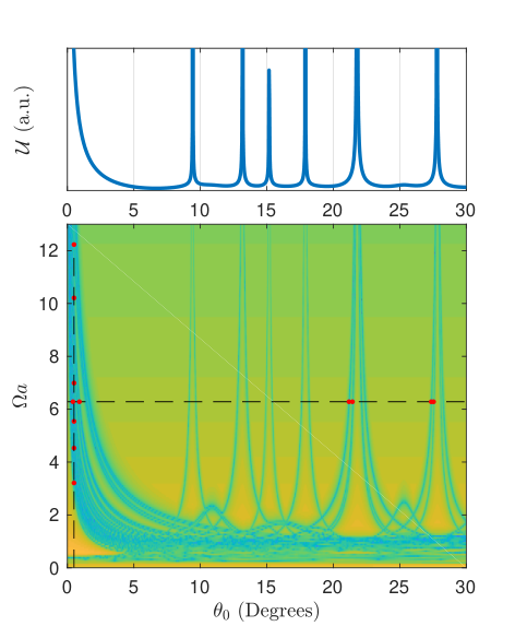
Figure 4 shows examples of the different modes found along the line , and marked in figure 3 as red dots in the horizontal line. Labeled from to , the patterns correspond to the rotation angles degrees. Mode corresponds to the excitation of dipoles due to a small rotation angle, while all the other modes correspond to the excitation of dipolar modes because of the commensurable phase of the cluster. Modes and are clearly paired and correspond to the excitation of dipoles in the same commensurable phase but at different distances due to the radial symmetry of the rotation, as explained before.

Figure 5 shows the different modes found at a fixed small rotation angle of , so that a large number of resonances is excited. Labeled from to , we show plots at frequencies . The modes are more and more interior to the cluster (except mode , probably a cluster mode). This variation is due to the fact that for a small rotation angle the distance between dipoles is radially increasing, therefore following the curve of figure 2 the wavelength of the corresponding mode will also be increasing with the distance to the center or the cluster and the frequency will be decreasing. This remarkable property shows how we can generate a large number of resonant modes for a small rotation angle, in opposite to what we have near the commensurable angles, where the number of frequencies is one or two for small clusters, though tunable with the rotation angle.

Finally, figure 6 shows the effect of the impedance term with the localization and number of modes. Results are shown for . For a high value of , which is the situation considered so far, the modes localize at small rotation angles and near the commensurable ones, as has been discussed before. However, decreasing the value of we find that, since the interaction between dipoles is weaker, the modes are more spread along the different angles. While we still can see a large number of these at special values of the rotation angle, their interpretation is however more complex since localization can be due to the interference between scattered waves, in a similar mechanism to “Anderson localization”Wiersma et al. 1997.
In summary, it has been found that the multiple scattering of waves between two nearby scatterers creates localized waves, so that when two lattices of scatterers are stacked and relatively twisted a large number of dipoles is formed and, consequently, a set of resonances appears. We have found that, for a fixed frequency, this set of resonances appears at special values of the rotation angle, which have been comprehensively explained in terms of multiple scattering theory . This work shows that, since the scatterers in the two lattices are closer each other than in the individual lattices, this effect should play a central role in the study of twisted bilayers, which have been deeply studied in condensed matter physics by coupling hamiltonians of the equivalent continuous layers. In the domain of phononics, where the lattices are artificial man-made structures and contain much less scattering units, it is obvious that the individual analysis presented here will be the dominant phenomenon. Finally, we believe that these structures are promising candidates for the realization of mechanically tunable wave-trapping devices, not only for their efficient functionality but also for the relatively easy design based on multiple scattering theory. Although numerical examples have been reported for flexural waves in thin elastic plates, the conclusions of this work can be applied to any kind of waves, including electronic waves.
Acknowledgements.
Daniel Torrent acknowledges financial support through the “Ramón y Cajal” fellowship under grant number RYC-2016-21188 and to the Ministry of Science, Innovation and Universities through Project No. RTI2018- 093921-A-C42. Marc Martí-Sabaté acknowledges financial support through the FPU program under grant number FPU18/02725.References
- Zeller and Günther (2014) P. Zeller and S. Günther, New Journal of Physics 16, 083028 (2014).
- Morell et al. (2010) E. S. Morell, J. Correa, P. Vargas, M. Pacheco, and Z. Barticevic, Physical Review B 82, 121407(R) (2010).
- Bistritzer and MacDonald (2011) R. Bistritzer and A. H. MacDonald, Proceedings of the National Academy of Sciences 108, 12233 (2011).
- San-Jose et al. (2012) P. San-Jose, J. Gonzalez, and F. Guinea, Physical review letters 108, 216802 (2012).
- Cao et al. (2018) Y. Cao, V. Fatemi, S. Fang, K. Watanabe, T. Taniguchi, E. Kaxiras, and P. Jarillo-Herrero, Nature 556, 43 (2018).
- Cao et al. (2020) Y. Cao, D. Chowdhury, D. Rodan-Legrain, O. Rubies-Bigorda, K. Watanabe, T. Taniguchi, T. Senthil, and P. Jarillo-Herrero, Physical Review Letters 124, 076801 (2020).
- Carr et al. (2017) S. Carr, D. Massatt, S. Fang, P. Cazeaux, M. Luskin, and E. Kaxiras, Physical Review B 95, 075420 (2017).
- Huang et al. (2016) C. Huang, F. Ye, X. Chen, Y. V. Kartashov, V. V. Konotop, and L. Torner, Scientific reports 6, 32546 (2016).
- Wang et al. (2020) P. Wang, Y. Zheng, X. Chen, C. Huang, Y. V. Kartashov, L. Torner, V. V. Konotop, and F. Ye, Nature 577, 42 (2020).
- Hu et al. (2020) G. Hu, Q. Ou, G. Si, Y. Wu, J. Wu, Z. Dai, A. Krasnok, Y. Mazor, Q. Zhang, Q. Bao, et al., Nature 582, 209 (2020).
- Jin et al. (2020) Y. Jin, W. Wang, Z. Wen, D. Torrent, and B. Djafari-Rouhani, Extreme Mechanics Letters p. 100777 (2020).
- Bouchitté et al. (2010) G. Bouchitté, S. Guenneau, and F. Zolla, Multiscale Modeling & Simulation 8, 1862 (2010).
- Tarnopolsky et al. (2019) G. Tarnopolsky, A. J. Kruchkov, and A. Vishwanath, Physical review letters 122, 106405 (2019).
- Foldy (1945) L. L. Foldy, Physical review 67, 107 (1945).
- Martin (2006) P. A. Martin, 107 (Cambridge University Press, 2006).
- Ochiai and Sánchez-Dehesa (2002) T. Ochiai and J. Sánchez-Dehesa, Physical Review B 65, 245111 (2002).
- Norris and Vemula (1995) A. Norris and C. Vemula, Journal of sound and vibration 181, 115 (1995).
- Torrent et al. (2014) D. Torrent, Y. Pennec, and B. Djafari-Rouhani, Physical Review B 90, 104110 (2014).
- Torrent et al. (2013) D. Torrent, D. Mayou, and J. Sánchez-Dehesa, Physical Review B 87, 115143 (2013).
- Packo et al. (2019) P. Packo, A. N. Norris, and D. Torrent, Physical Review Applied 11, 014023 (2019).
- Xiao et al. (2012) Y. Xiao, J. Wen, and X. Wen, Journal of Physics D: Applied Physics 45, 195401 (2012).
- Wiersma et al. (1997) D. S. Wiersma, P. Bartolini, A. Lagendijk, and R. Righini, Nature 390, 671 (1997).