: Probabilistic In-band Network TelemetryCCS: Networks Network protocolsCCS: Networks Network algorithmsCCS: Networks Network monitoring
Abstract.
Commodity network devices support adding in-band telemetry measurements into data packets, enabling a wide range of applications, including network troubleshooting, congestion control, and path tracing. However, including such information on packets adds significant overhead that impacts both flow completion times and application-level performance.
We introduce , an in-band telemetry framework that bounds the amount of information added to each packet. encodes the requested data on multiple packets, allowing per-packet overhead limits that can be as low as one bit. We analyze and prove performance bounds, including cases when multiple queries are running simultaneously. is implemented in P4 and can be deployed on network devices.Using real topologies and traffic characteristics, we show that concurrently enables applications such as congestion control, path tracing, and computing tail latencies, using only sixteen bits per packet, with performance comparable to the state of the art.
1. Introduction
Network telemetry is the basis for a variety of network management applications such as network health monitoring (Tammana et al. 2016), debugging (Guo et al. 2015), fault localization (Arzani et al. 2018), resource accounting and planning (Narayana et al. 2016), attack detection (Savage et al. 2000; Gkounis et al. 2016), congestion control (Li et al. 2019), load balancing (Alizadeh et al. 2014; Katta et al. 2016; Katta et al. 2017), fast reroute (Liu et al. 2013), and path tracing (Jeyakumar et al. 2014). A significant recent advance is provided by the In-band Network Telemetry (INT) (The P4.org Applications Working Group 11111). INT allows switches to add information to each packet, such as switch ID, link utilization, or queue status, as it passes by. Such telemetry information is then collected at the network egress point upon the reception of the packet.
INT is readily available in programmable switches and network interface cards (NICs) (Broadcom 11111; Barefoot 11111; Netronome 11111; Xilinx 11111c), enabling an unprecedented level of visibility into the data plane behavior and making this technology attractive for real-world deployments (Central 11111; Li et al. 2019). A key drawback of INT is the overhead on packets. Since each switch adds information to the packet, the packet byte overhead grows linearly with the path length. Moreover, the more telemetry data needed per-switch, the higher the overhead is: on a generic data center topology with 5 hops, requesting two values per switch requires 48 Bytes of overhead, or 4.8% of a 1000 bytes packet (§2). When more bits used to store telemetry data, fewer bits can be used to carry the packet payload and stay within the maximum transmission unit (MTU). As a result, applications may have to split a message, e.g., an RPC call, onto multiple packets, making it harder to support the run-to-completion model that high-performance transport and NICs need (Barbette et al. 2015). Indeed, the overhead of INT can impact application performance, potentially leading in some cases to a 25% increase and 20% degradation of flow completion time and goodput, respectively (§2). Furthermore, it increases processing latency at switches and might impose additional challenges for collecting and processing the data (§2).
We would like the benefits of in-band network telemetry, but at smaller overhead cost; in particular, we wish to minimize the per-packet bit overhead. We design Probabilistic In-band Network Telemetry (), a probabilistic variation of INT, that provides similar visibility as INT while bounding the per-packet overhead according to limits set by the user. allows the overhead budget to be as low as one bit, and leverages approximation techniques to meet it. We argue that often an approximation of the telemetry data suffices for the consuming application. For example, telemetry-based congestion control schemes like HPCC (Li et al. 2019) can be tuned to work with approximate telemetry, as we demonstrate in this paper. In some use cases, a single bit per packet suffices.
With , a query is associated with a maximum overhead allowed on each packet. The requested information is probabilistically encoded onto several different packets so that a collection of a flow’s packets provides the relevant data. In a nutshell, while with INT a query triggers every switch along the path to embed their own information, spreads out the information over multiple packets to minimize the per-packet overhead. The insight behind this approach is that, for most applications, it is not required to know all of the per-packet-per-hop information that INT collects. existing techniques incur high overheads due to requiring perfect telemetry information. For applications where some imperfection would be sufficient, these techniques may incur unnecessary overheads. Is designed for precisely such applications For example, it is possible to check a flow’s path conformance (Handigol et al. 2014; Tammana et al. 2016; Narayana et al. 2016), by inferring its path from a collection of its packets. Alternatively, congestion control or load balancing algorithms that rely on latency measurements gathered by INT, e.g., HPCC (Li et al. 2019), Clove (Katta et al. 2017) can work if packets convey information about the path’s bottleneck, and do not require information about all hops.
We present the framework (§3) and show that it can run several concurrent queries while bounding the per-packet bit overhead. To that end, uses each packet for a query subset with cumulative overhead within the user-specified budget. We introduce the techniques we used to build this solution (§4) alongside its implementation on commercial programmable switches supporting P4 (§5). Finally, we evaluate (§6) our approach with three different use cases. The first traces a flow’s path, the second uses data plane telemetry for congestion control, and the third estimates the experienced median/tail latency. Using real topologies and traffic characteristics, we show that enables all of them concurrently, with only sixteen bits per packet and while providing comparable performance to the state of the art.
In summary, the main contributions of this paper are:
- •
We present , a novel in-band network telemetry approach that provides fine-grained visibility while bounding the per-packet bit overhead to a user-defined value.
- •
We analyze and rigorously prove performance bounds.
- •
We evaluate in on path tracing, congestion control, and latency estimation, over multiple network topologies.
- •
We open source our code (cod 2020).
| Metadata value | Description |
|---|---|
| Switch ID | ID associated with the switch |
| Ingress Port ID | Packet input port |
| Ingress Timestamp | Time when packet is received |
| Egress Port ID | Packet output port |
| Hop Latency | Time spent within the device |
| Egress Port TX utilization | Current utilization of output port |
| Queue Occupancy | The observed queue build up |
| Queue Congestion Status | Percentage of queue being used |
2. INT and its Packet Overhead
INT is a framework designed to allow the collection and reporting of network data plane status at switches, without requiring any control plane intervention. In its architectural model, designated INT traffic sources, (e.g., the end-host networking stack, hypervisors, NICs, or ingress switches), add an INT metadata header to packets. The header encodes telemetry instructions that are followed by network devices on the packet’s path. These instructions tell an INT-capable device what information to add to packets as they transit the network. Table 1 summarizes the supported metadata values. Finally, INT traffic sinks, e.g., egress switches or receiver hosts, retrieve the collected results before delivering the original packet to the application. The INT architectural model is intentionally generic, and hence can enable a number of high level applications, such as (1) Network troubleshooting and verification, i.e., microburst detection (Jeyakumar et al. 2014), packet history (Handigol et al. 2014), path tracing (Jeyakumar et al. 2014), path latency computation (Ivkin et al. 2019); (2) Rate-based congestion control, i.e., RCP (Dukkipati and McKeown 2006), XCP (Katabi et al. 2002), TIMELY (Mittal et al. 2015); (3) Advanced routing, i.e, utilization-aware load balancing (Alizadeh et al. 2014; Katta et al. 2016).
INT imposes a non insignificant overhead on packets though. The metadata header is defined as an 8B vector specifying the telemetry requests. Each value is encoded with a 4B number, as defined by the protocol (The P4.org Applications Working Group 11111). As INT encodes per-hop information, the overall overhead grows linearly with both the number of metadata values and the number of hops. For a generic data center topology with 5 hops, the minimum space required on packet would be 28 bytes (only one metadata value per INT device), which is 2.8% of a 1000 byte packet (e.g., RDMA has a 1000B MTU). Some applications, such as Alibaba’s High Precision Congestion Control (Li et al. 2019) (HPCC), require three different INT telemetry values for each hop. Specifically, for HPCC, INT collects timestamp, egress port tx utilization, and queue occupancy, alongside some additional data that is not defined by the INT protocol. This would account for around 6.8% overhead using a standard INT on a 5-hop path.11 1 HPCC reports a slightly lower (4.2%) overhead because they use customized INT. For example, they do not use the INT header as the telemetry instructions do not change over time. This overhead poses several problems:
1. High packet overheads degrade application performance. The significant per-packet overheads from INT affect both flow completion time and application-level throughput, i.e., goodput. We ran an NS3 (The University of Washington NS-3 Consortium 11111) experiment to demonstrate this. We created a 5-hop fat-tree data center topology with 64 hosts connected through 10Gbps links. Each host generates traffic to randomly chosen destinations with a flow size distribution that follows a web search workload (Alizadeh et al. 2010). We employed the standard ECMP routing with TCP Reno. We ran our experiments with a range of packet overheads from 28B to 108B. The selected overheads correspond to a 5-hop topology, with one to five different INT values collected at each hop. Figure 2 shows the effect of increasing overheads on the average flow completion time (FCT) for 30% (average) and 70% (high) network utilization. Figure 2, instead, focuses on the goodput for only the long flows, i.e., with flow size >10 MBytes. Both graphs are normalized to the case where no overhead is introduced on packets.
| Application | Description | Measurement Primitives |
|---|---|---|
| Per-packet aggregation | ||
| Congestion Control (Katabi et al. 2002; Dukkipati and McKeown 2006; Han et al. 2013; Li et al. 2019) | Congestion Control with in-network support | timestamp, port utilization, queue occupancy |
| Congestion Analysis (Joshi et al. 2018; Chen et al. 2019; Narayana et al. 2017) | Diagnosis of short-lived congestion events | queue occupancy |
| Network Tomography (Geng et al. 2019) | Determine network state, i.e., queues status | switchID, queue occupancy |
| Power Management (Heller et al. 2010) | Determine under-utilized network elements | switchID, port utilization |
| Real-Time Anomaly Detection (Schweller et al. 2004; Yu et al. 2013) | Detect sudden changes in network status | timestamp, port utilization, queue occupancy |
| Static per-flow aggregation | ||
| Path Tracing (Savage et al. 2000; Jeyakumar et al. 2014; Tammana et al. 2016; Narayana et al. 2016) | Detect the path taken by a flow or a subset | switchID |
| Routing Misconfiguration (Snoeren et al. 2001; Tammana et al. 2016; Li et al. 2016) | Identify unwanted path taken by a given flow | switchID |
| Path Conformance (Li et al. 2016; Tammana et al. 2018; Snoeren et al. 2001) | Checks for policy violations. | switchID |
| Dynamic per-flow aggregation | ||
| Utilization-aware Routing (Alizadeh et al. 2014; Katta et al. 2016; Katta et al. 2017) | Load balance traffic based on network status. | switchID, port utilization |
| Load Imbalance (Li et al. 2016; Tammana et al. 2018; Savage et al. 2000) | Determine links processing more traffic. | switchID, port utilization |
| Network Troubleshooting (Jeyakumar et al. 2014; Narayana et al. 2017; Tammana et al. 2018) | Determine flows experiencing high latency. | switchID, timestamp |
In the presence of 48 bytes overhead, which corresponds to 3.2% of a 1500B packet (e.g., Ethernet has a 1500B MTU), the average FCT increases by 10%, while the goodput for long flows degrades by 10% if network utilization is approximately 70%. Further increasing the overhead to 108B (7.2% of a 1500B packet) leads to a 25% increase and 20% degradation of flow completion time and goodput, respectively. This means that even a small amount of bandwidth headroom can provide a dramatic reduction in latency (Alizadeh et al. 2012). The long flows’ average goodput is approximately proportional to the residual capacity of the network. That means, at a high network utilization, the residual capacity is low, so the extra bytes in the header cause larger goodput degradation than the byte overhead itself (Alizadeh et al. 2012). As in our example, the theoretical goodput degradation should be around when increasing the header overhead from 48B to 108B at around 70% network utilization. This closely matches the experiment result, and is much larger than the extra byte overhead (4%).
Although some data center networks employ jumbo frames to mitigate the problem22 2 https://docs.aws.amazon.com/AWSEC2/latest/UserGuide/network_mtu.html, it is worth noting that (1) not every network can employ jumbo frames, especially the large number of enterprise and ISP networks; (2) some protocols might not entirely support jumbo frames; for example, RDMA over Converged Ethernet NICs provides an MTU of only 1KB (Mittal et al. 2018).
2. Switch processing time. In addition to consuming bandwidth, the INT overhead also affects packet processing time at switches. Every time a packet arrives at and departs from a switch, the bits carried over the wire need to be converted from serial to parallel and vice versa, using the 64b/66b (or 66b/64b) encoding as defined by the IEEE Standard 802.3 (IEEE 11111). For this reason, any additional bit added into a packet affects its processing time, delaying it at both input and output interfaces of every hop. For example, adding 48 bytes of INT data on a packet (INT header alongside two telemetry information) would cause a latency increase with respect to the original packet of almost and for 10G and 100G interfaces, respectively33 3 Consuming 48Bytes on a 10G interface requires 6 clock cycles each of them burning 6.4 ns (Xilinx 11111a). On a 100G interface, it needs just one clock cycle of 3ns (Xilinx 11111b).. On a state-of-the-art switch with 10G interfaces, this can represent an approximately 3% increase in processing latency (Oudin et al. 2019). On larger topologies and when more telemetry data is needed, the overhead on the packet can cause an increase of latency in the order of microseconds, which can hurt the application performance (Popescu et al. 2017).
3. Collection overheads. Telemetry systems such as INT generate large amounts of traffic that may overload the network. Additionally, INT produces reports of varying size (depending on the number of hops), while state-of-the-art end-host stack processing systems for telemetry data, such as Confluo (Khandelwal et al. 2019), rely on fixed-byte size headers on packets to optimize the computation overheads.
3. The Framework
We now discuss the supported functionalities of our system, formalizing the model it works in.
Telemetry Values. In our work, we refer to the telemetry information as values. Specifically, whenever a packet reaches a switch , we assume that the switch observes a value . The value can be a function of the switch (e.g., port or switch ID), switch state (e.g., timestamp, latency, or queue occupancy), or any other quantity computable in the data plane. In particular, our definition supports the information types that INT (The P4.org Applications Working Group 11111) can collect.
3.1. Aggregation Operations
We design with the understanding that collecting all (per-packet per-switch) values pose an excessive and unnecessary overhead. Instead, supports several aggregation operations that allow efficient encoding of the aggregated data onto packets. For example, congestion control algorithms that rely on the bottleneck link experienced by packets (e.g., (Li et al. 2019)) can use a per-packet aggregation. Alternatively, applications that require discovering the flow’s path (e.g., path conformance) can use per-flow aggregation.
- •
Per-packet aggregation summarizes the data across the different values in the packet’s path, according to an aggregation function (e.g., max/min/sum/product). For example, if the packet traverses the switches and we perform a max-aggregation, the target quantity is .
- •
Static per-flow aggregation targets summarizing values that may differ between flows or switches, but are fixed for a (flow, switch) pair. Denoting the packets of flow by , the static property means that for any switch on ’s path we have ; for convenience, we denote . If the path taken by is , the goal of this aggregation is then to compute all values on the path, i.e., . As an example, if is the ID of the switch , then the aggregation corresponds to inferring the flow’s path.
- •
Dynamic per-flow aggregation summarizes, for each switch on a flow’s path, the stream of values observed by its packets. Denote by the packets of and by its path, and let sequence of values measured by on ’s packets be denoted as . The goal is to compute a function of according to an aggregation function (e.g., median or number of values that equal a particular value ). For example, if is the latency of the packet on the switch , using the median as an aggregation function equals computing the median latency of flow on .
3.2. Use Cases
can be used for a wide variety of use cases (see Table 2). In this paper, we will mainly discuss three of them, chosen in such a way that we can demonstrate all the different aggregations in action.
Per-packet aggregation: Congestion Control. State of the art congestion control solutions often use INT to collect utilization and queue occupancy statistics (Li et al. 2019). shows that we can get similar or better performance while minimizing the overheads associated with collecting the statistics.
Static per-flow aggregation: Path Tracing. Discovering the path taken by a flow is essential for various applications like path conformance (Li et al. 2016; Tammana et al. 2018; Snoeren et al. 2001). In , we leverage multiple packets from the same flow to infer its path. For simplicity, we assume that each flow follows a single path.
Dynamic per-flow aggregation: Network Troubleshooting. For diagnosing network issues, it is useful to measure the latency quantiles from each hop (Jeyakumar et al. 2014; Narayana et al. 2017; Chen et al. 2019; Ivkin et al. 2019). Tail quantiles are reported as the most effective way to summarize the delay in an ISP (Choi et al. 2007). For example, we can detect network events in real-time by noticing a change in the hop latency (Barefoot Networks 2018). To that end, we leverage to collect the median and tail latency statistics of (switch, flow) pairs.
3.3. Query Language
Each query in is defined as a tuple that specifies
which values are used (e.g., switch IDs or latency), the aggregation type as in Section 3.1, and the query bit-budget (e.g., bits per packet). The user may also specify a space-budget that determines how much per-flow storage is allowed, the flow-definition (e.g., 5-tuple, source IP, etc.) in the case of per-flow queries,
and the query frequency (that determines which fraction of the packets should be allocated for the query).
works with static bit-budgets to maximize its effectiveness while remaining transparent to the sender and receiver of a packet. Intuitively, when working with INT/PINT one needs to ensure that a packet’s size will not exceed the MTU even after the telemetry information is added. For example, for a 1500B network MTU, if the telemetry overhead may add to bytes, then the sender would be restricted to sending packets smaller than 1500. Thus, by fixing the budget, we allow the network flows to operate without being aware of the telemetry queries and path length.
3.4. Query Engine
allows the operator to specify multiple queries that should run concurrently and a global bit-budget. For example, if the global bit-budget is bits, we can run two -bit-budget queries on the same packet. In , we add to packets a digest – a short bitstring whose length equals the global bit budget. This digest may compose of multiple query digests as in the above example.

Each query instantiates an Encoding Module, a Recording Module, and an Inference Module. The Encoding runs on the switches and modifies the packet’s digest. When a packet reaches a Sink (the last hop on its path), the sink extracts (removes) the digest and sends the data packet to its destination. This way, remains transparent to both the sender and receiver. The extracted digest is intercepted by the Recording Module, which processes and stores the digests. We emphasize that the per-flow data stored by the Recording Module sits in an offline storage and no per-flow state is stored on the switches. Another advantage of is that, compared with INT, we send fewer bytes from the sink to be analyzed and thereby reduce the network overhead. The Inference Module runs on a commodity server that uses the stored data to answer queries. Fig. 3 illustrates ’s architecture.
Importantly, all switches must agree on which query set to run on a given packet, according to the distribution chosen by the Query Engine. We achieve coordination using a global hash function, as described in Section 4.1. Unlike INT, we do not add a telemetry header; in this way we minimize the bit overhead.44 4 We note that removing the header is minor compared to the overhead saving obtains by avoiding logging all per-hop values. Instead, the Query Engine compiles the queries to decide on the execution plan (which is a probability distribution on a query set, see Fig. 3) and notifies the switches.
3.5. Challenges
We now discuss several challenges we face when designing algorithms for .
Bit constraints. In some applications, the size of values may be prohibitively large to a point where writing a single value on each packet poses an unacceptable overhead.
Switch Coordination. The switches must agree on which query set to use for each packet. While the switches can communicate by exchanging bits that are added to packets, this increases the bit-overhead of and should be avoided.
Switch constraints. The hardware switches have constraints, including limited operations per packet, limited support for arithmetic operations (e.g., multiplication is not supported), inability to keep per-flow state, etc. See (Ben-Basat et al. 2018) for a discussion of the constraints. For , these constraints mean that we must store minimal amount of state on switches and use simple encoding schemes that adhere to the programmability restrictions.
4. Aggregation Techniques
In this section, we present the techniques used by to overcome the above challenges. We show how global hash functions allow efficient coordination between different switches and between switches and the Inference Module. We also show how distributed encoding schemes help reduce the number of packets needed to collect the telemetry information. Finally, we adopt compression techniques to reduce the number of bits required to represent numeric values (e.g., latency).
Our techniques reduce the bit-overhead on packets using probabilistic techniques. As a result, some of our algorithms (e.g., latency quantile estimation) are approximate, while others (e.g., path tracing) require multiple packets from the same flow to decode. Intuitively, oftentimes one mostly cares about tracing large (e.g., malicious) flows and does not require discovering the path of very short ones. Similarly, for network diagnostics it is OK to get approximated latency measurements as we usually care about large latencies or significant latency changes. We summarize which techniques apply for each of the use cases in Table 3.
| Use Case | Global Hashes | Distributed Coding | Value Approximation |
|---|---|---|---|
| Congestion Control | ✗ | ✗ | ✓ |
| Path Tracing | ✓ | ✓ | ✗ |
| Latency Quantiles | ✓ | ✗ | ✓ |
4.1. Implicit Coordination via Global Hash Functions
In , we extensively use global hash functions to determine probabilistic outcomes at the switches. As we show, this solves the switch coordination challenge, and also enables implicit coordination between switches and the Inference Module – a feature that allows us to develop efficient algorithms.
Coordination among switches. We use a global (i.e., that is known to all switches) hash function to determine which query set the current packet addresses. For example, suppose that we have three queries, each running with probability , and denote the query-selection hash, mapping packet IDs to the real interval55 5 For simplicity, we consider hashing into real numbers. In practice, we hash into bits (the range ) for some integer (e.g., ). Checking if the real-valued hash is in corresponds to checking if the discrete hash is in the interval . , by . Then if , all switches would run the first query, if the second query, and otherwise the third. Since all switches compute the same , they agree on the executed query without communication. This approach requires the ability to derive unique packet identifiers to which the hashes are applied (e.g., IPID, IP flags, IP offset, TCP sequence and ACK numbers, etc.). For a discussion on how to obtain identifiers, see (Duffield and Grossglauser 2001).
Coordination between switches and Inference Module. The Inference Module must know which switches modified an incoming packet’s digest, but we don’t want to spend bits on encoding switch IDs in the packet. Instead, we apply a global hash function on a (packet ID, hop number)66 6 The hop number can be computed from the current TTL on the packet’s header. pair to choose whether to act on a packet. This enables the Recording Module to compute ’s outcome for all hops on a packet’s path and deduct where it was modified. This coordination plays a critical role in our per-flow algorithms as described below.
Example #1: Dynamic Per-flow aggregation. In this aggregation, we wish to collect statistics from values that vary across packets, e.g., the median latency of a (flow, switch) pair. We formulate the general problem as follows: Fix some flow . Let denote the packets of and denote its path. For each switch , we need to collect enough information about the sequence while meeting the query’s bit-budget. For simplicity of presentation, we assume that packets can store a single value.77 7 If the global bit-budget does not allow encoding a value, we compress it at the cost of an additional error as discussed in Section 4.3. If the budget allows storing multiple values, we can run the algorithm independently multiple times and thereby collect more information to improve the accuracy.
’s Encoding Module runs a distributed sampling process. The goal is to have each packet carry the value of a uniformly chosen hop on the path. That is, each packet should carry each value from with probability . This way, with probability , each hop will get samples, i.e., almost an equal number.
To get a uniform sample, we use a combination of global hashing and the Reservoir Sampling algorithm (Vitter 1985). Specifically, when the ’th hop on the path (denoted ) sees a packet , it overwrites its digest with if . Therefore, the packet will end up carrying the value only if (i) , and (ii) . To get uniform sampling, we follow the Reservoir Sampling algorithm and set . Indeed, for each hop (i) and (ii) are simultaneously satisfied with probability . Intuitively, while later hops have a lower chance of overriding the digest, they are also less likely to be replaced by the remaining switches along the path.
Intuitively, we can then use existing algorithms for constructing statistics from subsampled streams. That is, for each switch , the collected data is a uniformly subsampled stream of . One can then apply different aggregation functions. For instance, we can estimate quantiles and find frequently occurring values. As an example, we can estimate the median and tail latency of the (flow, switch) pair by finding the relevant quantile of the subsampled stream.
On the negative side, aggregation functions like the number of distinct values or the value-frequency distribution entropy are poorly approximable from subsampled streams (Mcgregor et al. 2016).
aims to minimize the decoding time and amount of per-flow storage. To that end, our Recording Module does not need to store all the incoming digests. Instead, we can use a sketching algorithm that suits the target aggregation (e.g., a quantile sketch (Karnin et al. 2016)). That is, for each switch through which flow is routed, we apply a sketching algorithm to the sampled substream of . If given a per-flow space budget (see §3.3) we split it between the sketches evenly. This allows us to record a smaller amount of per-flow information and process queries faster. Further, we can use a sliding-window sketch (e.g., (Arasu and Manku 2004; Basat et al. 2018; Ben-Basat et al. 2018)) to reflect only the most recent measurements. Finally, the Inference Module uses the sketch to provide estimates on the required flows.
The accuracy of for dynamic aggregation depends on the aggregation function, the number of packets , the length of the path , and the per-flow space stored by the Recording Module (which sits off-switch in remote storage). We state results for two typical aggregation functions. The analysis is deferred to Section A.1.
Theorem 1.
Fix an error target and a target quantile (e.g., is the median). After seeing packets from a flow , using space, produces a -quantile of for each hop .
Theorem 2.
Fix an error target and a target threshold . After seeing packets from a flow , using space, produces all values that appear in at least a -fraction of , and no value that appears less than a -fraction, for each hop .
4.2. Distributed Coding Schemes
When the values are static for a given flow (i.e., do not change between packets), we can improve upon the dynamic aggregation approach using distributed encoding. Intuitively, in such a scenario, we can spread each value over multiple packets. The challenge is that the information collected by is not known to any single entity but is rather distributed between switches. This makes it challenging to use existing encoding schemes as we wish to avoid adding extra overhead for communication between switches. Further, we need a simple encoding scheme to adhere to the switch limitations, and we desire one that allows efficient decoding.
Traditional coding schemes assume that a single encoder owns all the data that needs encoding. However, in , the data we wish to collect can be distributed among the network switches. That is, the message we need to transfer is partitioned between the different switches along the flow’s path.
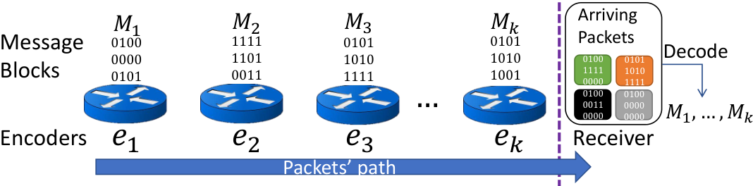
We present an encoding scheme that is fully distributed without any communication between encoders. Specifically, we define our scheme as follows: a sequence of encoders hold a -block message such that encoder has for all . The setting is illustrated in Fig. 4. Each packet carries a digest which has a number of bits that equals the block size and has a unique identifier which distinguishes it from other packets. Additionally, each encoder is aware of its hop number (e.g., by computing it from the TTL field in the packet header). The packet starts with a digest of (a zero bitstring) and passes through . Each encoder can modify the packet’s digest before passing it to the next encoder. After the packet visits , it is passed to the Receiver, which tries to decode the message. We assume that the encoders are stateless to model the switches’ inability to keep a per-flow state in networks.
Our main result is a distributed encoding scheme that needs packets for decoding the message with near-linear decoding time. We note that Network Coding (Ho et al. 2003) can also be adapted to this setting. However, we have found it rather inefficient, as we explain later on.
Baseline Encoding Scheme. A simple and intuitive idea for a distributed encoding scheme is to carry a uniformly sampled block on each packet. That is, the encoders can run the Reservoir Sampling algorithm using a global hash function to determine whether to write their block onto the packet. Similarly to our Dynamic Aggregation algorithm, the Receiver can determine the hop number of the sampling switch, by evaluating the hash function, and report the message.
The number of packets needed for decoding the message using this scheme follows the Coupon Collector Process (e.g., see (Flajolet et al. 1992)), where each block is a coupon and each packet carries a random sample. It is well-known that for coupons, we would need samples on average to collect them all. For example, for , Coupon Collector has a median (i.e., probability of 50% to decode) of packets and a 99’th percentile of packets, as shown in Fig. 5.
The problem with the Baseline scheme is that while the first blocks are encoded swiftly, later ones require a higher number of packets. The reason is that after seeing most blocks, every consecutive packet is unlikely to carry a new block. This is because the encoders are unaware of which blocks were collected and the probability of carrying a new block is proportional to number of missing blocks. As a result, the Baseline scheme has a long “tail”, meaning that completing the decoding requires many packets.
Distributed XOR Encoding. An alternative to the Baseline scheme is to use bitwise-xor while encoding. We avoid assuming that the encoders know , but assume that they know a typical length , such that . Such an assumption is justified in most cases; for example, in data center topologies we often know a tight bound on the number of hops (Tammana et al. 2016). Alternatively, the median hop count in the Internet is estimated to be (Van Mieghem et al. 2001), while only a few paths have more than hops (Theilmann and Rothermel 2000; Carter and Crovella 1997). The XOR encoding scheme has a parameter , and each encoder on the path bitwise-xors its message onto the packet’s digest with probability , according to the global hash function. That is, the ’th encoder changes the digest if . We note that this probability is uniform and that the decision of whether to xor is independent for each encoder, allowing a distributed implementation without communication between the encoders.
When a packet reaches the Receiver, the digest is a bitwise-xor of multiple blocks , where is a binomial random variable . The Receiver computes to determine the values . If this set contains exactly one unknown message block, we can discover it by bitwise-xoring the other blocks. For example, if we have learned the values of and the current digest is , we can derive since .
On its own, the XOR encoding does not asymptotically improve over the Baseline. Its performance is optimized when , where it requires packets to decode, i.e., within a constant factor from the Baseline’s performance. Interestingly, we show that the combination of the two approaches gives better results.
Interleaving the Encoding Schemes. Intuitively, the XOR and Baseline schemes behave differently. In the Baseline, the chance of learning the value of a message block with each additional packet decreases as we receive more blocks. In contrast, to recover data from an XOR packet, we need to know all xor-ed blocks but one. When is much larger than , many packet digests are modified by multiple encoders, which means that the probability to learn a message block value increases as we decode more blocks.
As an example for how the interleaved scheme helps, consider the case of encoders. The Baseline scheme requires three packets to decode the message in expectation; the first packet always carries an unknown block, but each additional packet carries the missing block with probability only . In contrast, suppose each packet chooses the Baseline scheme and the XOR scheme each with probability , using . For the interleaved scheme to complete, we need either two Baseline packets that carry different blocks or one XOR packet and one Baseline packet. A simple calculation shows that this requires just packets in expectation.
For combining the schemes, we first choose whether to run the Baseline with probability , or the XOR otherwise. Once again, switches make the decision based on a global hash function applied to the packet identifier to achieve implicit agreement on the packet type. Intuitively, the Baseline scheme should reduce the number of undecoded blocks from to , and the XOR will decode the rest. To minimize the number of packets, we can set and the XOR probability88 8 If then ; in this case we set the probability to . to to reduce the required number of packets to ). In such setting, the Baseline decodes most hops, leaving for the XOR layer. For example, when , we get a median of packets and a 99’th percentile of packets to decode the message. That is, not only does it improve the average case, the interleaving has sharper tail bounds. This improvement is illustrated in Fig. 5.
Multi-layer Encoding. So far, we used a single probability for xor-ing each packet, which was chosen inversely proportional to (the number of hops that were not decoded by the Baseline scheme). This way, we maximized the probability that a packet is xor-ed by exactly one of these blocks, and we xor any block from the that are known already to remove them from the decoding. However, when most of the blocks left for XOR are decoded, it also “slows down” and requires more packets for decoding each additional block. Therefore, we propose to use multiple XOR layers that vary in their sampling probabilities. We call the Baseline scheme layer , and the XOR layers . Each XOR layer starts with undecoded blocks, xors with probability , and ends when blocks are undecoded.
Our analysis, given in Section A.2, shows that by optimizing the algorithm parameters and , we obtain the following result. The value of is a function of , and we have that if and if ; i.e., in practice we need only one or two XOR layers.
Theorem 3.
After seeing packets, the Multi-layer scheme can decode the message.
We note that the term hides an packets additive term, where the constant depends on how well approximates . Namely, when , our analysis indicates that packets are enough. Finally, we note that if is not representative of at all, we still get that packets are enough, the same as in the Baseline scheme (up to lower order terms). The reason is that our choice of is close to , i.e., only a small fraction of the packets are used in the XOR layers.
Comparison with Linear Network Coding. Several algorithms can be adapted to work in the distributed encoding setting. For example, Linear Network Coding (LNC) (Ho et al. 2003) allows one to decode a message in a near-optimal number of packets by taking random linear combinations over the message blocks. That is, on every packet, each block is xor-ed into its digest with probability . Using global hash functions to select which blocks to xor, one can determine the blocks that were xor-ed onto each digest. LNC requires just packets to decode the message. However, in some cases, LNC may be suboptimal and can use alternative solutions. First, the LNC decoding algorithm requires matrix inversion which generally takes time in practice (although theoretically faster algorithms are possible). If the number of blocks is large, we may opt for approaches with faster decoding. Second, LNC does not seem to work when using hashing to reduce the overhead. As a result, in such a setting, LNC could use fragmentation, but may require a larger number of packets than the XOR-based scheme using hashing.
Example #2: Static Per-flow Aggregation. We now discuss how to adapt our distributed encoding scheme for ’s static aggregation. Specifically, we present solutions that allow us to reduce the overhead on packets to meet the bit-budget in case a single value cannot be written on a packet. For example, for determining a flow’s path, the values may be -bit switch IDs, while the bit-budget can be smaller (even a single bit per packet). We also present an implementation variant that allows to decode the collection of packets in near-linear time. This improves the quadratic time required for computing for all packets and hops .
Reducing the Bit-overhead using Fragmentation. Consider a scenario where each value has bits while we are allowed to have smaller -bits digests on packets. In such a case, we can break each value into fragments where each has bits. Using an additional global hash function, each packet is associated with a fragment number in . We can then apply our distributed encoding scheme separately on each fragment number. While fragmentation reduces the bit overhead, it also increases the number of packets required for the aggregation, and the decode complexity, as if there were hops.
Reducing the Bit-overhead using Hashing. The increase in the required number of packets and decoding time when using fragmentation may be prohibitive in some applications. We now propose an alternative that allows decoding with fewer packets, if the value-set is restricted. Suppose that we know in advance a small set of possible block values , such that any is in . For example, when determining a flow’s path, can be the set of switch IDs in the network. Intuitively, the gain comes from the fact that the keys may be longer than bits (e.g., switch IDs are often 32-bit long, while networks have much fewer than switches). Instead of fragmenting the values to meet the -bits query bit budget, we leverage hashing. Specifically, we use another global hash function that maps (value, packet ID) pairs into -bit bitstrings. When encoder sees a packet , if it needs to act it uses to modify the digest. In the Baseline scheme will write on , and in the XOR scheme it will xor onto its current digest. As before, the Recording Module checks the hop numbers that modified the packet. The difference is in how the Inference Module works – for each hop number , we wish to find a single value that agrees with all the Baseline packets from hop . For example, if and were Baseline packets from hop , must be a value such that and . If there is more than one such value, the inference for the hop is not complete and we require additional packets to determine it. Once a value of a block is determined, from any digest that was xor-ed by the ’th encoder, we xor from . This way, the number of unknown blocks whose hashes xor-ed decreases by one. If only one block remains, we can treat it similarly to a Baseline packet and use it to reduce the number of potential values for that block. Another advantage of the hashing technique is that it does not assume anything about the width of the values (e.g., switch IDs), as long as each is distinct.
Reducing the Decoding Complexity. Our description of the encoding and decoding process thus far requires processing is super-quadratic () in . That is because we need packets to decode the message, and we spend time per packet in computing the function to determine which encoders modified its digest. We now present a variant that reduces the processing time to nearly linear in . Intuitively, since the probability of changing a packet is , the number of random bits needed to determine which encoders modify it is . Previously, each encoder used the global function to get pseudo-random bits and decide whether to change the packet. Instead, we can use to create pseudo-random -bit vectors. Intuitively, each bit in the bitwise-and of these vectors will be set with probability (as defined by the relevant XOR layer). The ’th encoder will modify the packet if the ’th bit is set in the bitwise-and of the vectors99 9 This assumes that the probability is a power of two, or provides a approximation of it. By repeating the process we can get a better approximation.. At the Recording Module, we can compute the set of encoders that modify a packet in time by drawing the random bits and using their bitwise-and. Once we obtain the bitwise-and vector we can extract a list of set bits in time using bitwise operations. Since the average number of set bits is , the overall per-packet complexity remains and the total decoding time becomes . We note that this improvement assumes that fits in machine words (e.g., ) and that encoders can do operations per packet.
Improving Performance via Multiple Instantiations. The number of packets needs to decode the message depends on the query’s bit-budget. However, increasing the number of bits in the hash may not be the best way to reduce the required number of packets. Instead, we can use multiple independent repetitions of the algorithm. For example, given an -bit query budget, we can use two independent -bit hashes.
4.3. Approximating Numeric Values
Encoding an exact numeric value on packet may require too many bits, imposing an undesirable overhead. For example, the 32-bit latency measurements that INT collects may exceed the bit-budget. We now discuss to compress the value, at the cost of introducing an error.
Multiplicative approximation. One approach to reducing the number of bits required to encode a value is to write on the packet’s digest instead of . Here, the operator rounds the quantity to the closest integer. At the Inference Module, we can derive a -approximation of the original value by computing . For example, if we want to compress a -bit value into bits, we can set .
Additive approximation. If distinguishing small values is not as crucial as bounding the maximal error, we obtain better results by encoding the value with additive error instead of multiplicative error. For a given error target (thereby reducing the overhead by bits), the Encoding Module writes , and the Inference Module computes .
Randomized counting. For some aggregation functions, the aggregation result may require more bits than encoding a single value. For example, in a per-packet aggregation over a -hop path with -bit values, the sum may require bits to write explicitly while the product may take bits. This problem is especially evident if is small (e.g., a single bit specifying whether the latency is high). Instead, we can take a randomized approach to increase the value written on a packet probabilistically. For example, we can estimate the number of high-latency hops or the end-to-end latency to within a -multiplicative factor using bits (Morris 1978).
Example #3: Per-packet aggregation. Here, we wish to summarize the data across the different values in the packet’s path. For example, HPCC (Li et al. 2019) collects per-switch information carried by INT data, and adjusts the rate at the end host according to the highest link utilization along the path. To support HPCC with , we have two key insights: (1) we just need to keep the highest utilization (i.e., the bottleneck) in the packet header, instead of every hop; (2) we can use the multiplicative approximation to further reduce the number of bits for storing the utilization. Intuitively, improves HPCC as it reduces the overheads added to packets, as explained in Section 2.
In each switch, we calculate the utilization as in HPCC, with slight tuning to be supported by switches (discussed later). The multiplication is calculated using log and exp based on lookup tables (Sharma et al. 2017). The result is encoded using multiplicative approximation. To further eliminate systematic error, we write , the randomly performs floor or ceiling, with a probability distribution that gives an expected value equals to . This way, some packets will overestimate the utilization while others underestimate it, thus resulting in the correct value on average. In practice, we just need 8 bits to support .
Tuning HPCC calculation for switch computation. We maintain the exponential weighted moving average (EWMA) of link utilization of each link in the switch. is updated on every packet with: , where is the new sample for updating . Here, is the base RTT and is the link bandwidth (both are constants). Intuitively, the weight of the EWMA, , corresponds to each new packet’s time occupation . The calculation of also corresponds to each new packet: is the packet’s size, and is the queue length when the packet is dequeued1010 10 This is slightly different from HPCC, where the calculation is done in the host, which can only see packets of its own flow. Therefore, the update is scaled for packets of the same flow ( is time gap between packets of the same flow, and includes the bytes from other flows in between). Here, the update is performed on all packets on the same link. Since different flows may interleave on the link, our calculation is more fine-grained..
To calculate the multiplications, we first do the following transformation: . Then we calculate the multiplications using logarithm and exponentiation as detailed in Appendix B.
5. Implementation
is implemented using the P4 language and can be deployed on commodity programmable switches. We explain how each of our use cases is executed.
For running the path tracing application (static per-flow aggregation), we require four pipeline stages. The first chooses a layer, another computes , the third hashes the switch ID to meet the query’s bit budget, and the last writes the digest. If we use more than one hash for the query, both can be executed in parallel as they are independent.
Computing the median/tail latency (dynamic per-flow aggregation) also requires four pipeline stages: one for computing the latency, one for compressing it to meet the bit budget; one to compute ; and one to overwrite the value if needed.
Our adaptation of the HPCC congestion control algorithm requires six pipeline stages to compute the link utilization, followed by a stage for approximating the value and another to write the digest. For completeness, we elaborate on how to implement in the data plane the different arithmetic operations needed by HPCC in Appendix C. We further note that running it may require that the switch would need to perform the update of in a single stage. In other cases, we propose to store the last values of on separate stages and update them in a round-robin manner, for some integer . This would mean that our algorithm would need to recirculate every ’th packet as the switch’s pipeline is one-directional.
Since the switches have a limited number of pipeline stages, we parallelize the processing of queries as they are independent of each other. We illustrate this parallelism for a combination of the three use cases of .We start by executing all queries simultaneously, writing their results on the packet vector. Since HPCC requires more stages than the other use cases, we concurrently compute which query subset to run according to the distribution selected by the Query Engine (see §3.4). We can then write the digests of all the selected queries without increasing the number of stages compared with running HPCC alone. The switch layout for such a combination is illustrated in Fig. 6.
6. Evaluation
We evaluate on the three use cases discussed on §3.2.
6.1. Congestion Control
We evaluate how affects the performance of HPCC (Li et al. 2019) using the same simulation setting as in (Li et al. 2019). Our goal is not to propose a new congestion control scheme, but rather to present a low-overhead approach for collecting the information that HPCC utilizes. We use NS3 (The University of Washington NS-3 Consortium 11111) and a FatTree topology with 16 Core switches, 20 Agg switches, 20 ToRs, and 320 servers (16 in each rack). Each server has a single 100Gbps NIC connected to a single ToR. The capacity of each link between Core and Agg switches, as well as Agg switches and ToRs, are all 400Gbps. All links have a 1s propagation delay, which gives a 12s maximum base RTT. The switch buffer size is 32MB. The traffic is generated following the flow size distribution in web search from Microsoft (Alizadeh et al. 2010) and Hadoop from Facebook (Roy et al. 2015). Each server generates new flows according to a Poisson process, destined to random servers. The average flow arrival time is set so that the total network load is 50% (not including the header bytes). We use the recommended setting for HPCC: bytes, , , and s.
The results, depicted in Fig. 7(b) and Fig. 7(c), show that has similar performance (in terms of slowdown) to HPCC, despite using just bits per packet. Here, slowdown refers to the ratio between the completion time of the flow in the presence of other flows and alone. Specifically, has better performance on long flows while slightly worse performance on short ones. The better performance on long flows is due to ’s bandwidth saving. Fig. 7(a) shows the relative goodput improvement, averaged over all flows over 10MB, of using at different network load. At higher load, the byte saving of brings more significant improvement. For example, at 70% load, using improves the goodput by 71%. This trend aligns with our observation in §2.
To evaluate how the congestion control algorithm would perform alongside other queries, we experiment in a setting where only a fraction of the packets carry the query’s digest. As shown in Fig. 8(a) and Fig. 8(b), the performance only slightly degrades for . This is expected, because the bandwidth-delay product (BDP) is 150 packets, so there are still 9.4 (150/16) packets per RTT carrying feedback. Thus the rate is adjusted on average once per 1/9.4 RTT (as compared to 1/150 RTT with per-packet feedback), which is still very frequent. With , the performance of short flows degrades significantly, because it takes longer than an RTT to get feedback. The implication is that congestion caused by long flows is resolved slowly, so the queue lasts longer, resulting in higher latency for short flows. The very long flows (e.g., > 5MB) also have worse performance. The reason is that they are long enough to collide with many shorter flows, so when the competing shorter flows finish, the long flows have to converge back to the full line rate. With , it takes much longer time to converge than with smaller .
In principle, the lower feedback frequency only affects the convergence speed as discussed above, but not the stability and fairness. Stability is guaranteed by no overreaction, and HPCC’s design of reference window (constant over an RTT) provides this regardless of . Fairness is guaranteed by additive-increase-multiplicative-decrease (AIMD), which is preserved regardless of .
6.2. Latency Measurements
Using the same topology and workloads as in our congestion control experiments, we evaluate ’s performance on estimating latency quantiles. We consider in four scenarios, using and bit-budgets, with sketches (denoted S), and without. In our experiment, we have used the, state of the art, KLL sketch (Karnin et al. 2016). The results, appearing in Fig. 9, show that when getting enough packets, the error of the aggregation becomes stable and converges to the error arising from compressing the values. As shown, by compressing the incoming samples using a sketch (e.g., that keeps identifiers regardless of the number of samples), accuracy degrades only a little even for small B sketches. We conclude that such sketches offer an attractive space to accuracy tradeoff.
6.3. Path Tracing
We conduct these experiments on Mininet (Mininet 11111) using two large-diameter (denoted ) ISP topologies (Kentucky Datalink and US Carrier) from Topology Zoo (Knight et al. 2011) and a () Fat Tree topology. The Kentucky Datalink topology consisted of 753 switches with a diameter of 59 and the US carrier topology consisted of 157 switches with a diameter of 36. For each topology and every path, we estimate the average and 99’th percentile number of packets needed for decoding over 10K runs. We consider three variants of – using 1-bit, 4-bit, and two independent 8-bit hash functions (denoted by ). We compare to two state-of-the-art IP Traceback solutions PPM (Savage et al. 2000) and AMS2 (Song and Perrig 2001) with and . When configured with , AMS2 requires more packets to infer the path but also has a lower chance of false positives (multiple possible paths) compared with . We implement an improved version of both algorithms using Reservoir Sampling, as proposed in (Sattari 2007). is configured with on the ISP topologies and (as this is the diameter) on the fat tree topology. In both cases, this means a single XOR layer in addition to a Baseline layer.
The results (Fig. 10) show that significantly outperforms previous works, even with a bit-budget of a single bit (PPM and AMS both have an overhead of bits per packet). As shown, the required number of packets for grows near-linearly with the path length, validating our theoretical analysis. For the Kentucky Datalink topology (), with on average uses 25–36 times fewer packets when compared to competing approaches. Even when using with , needs 7–10 times fewer packets than competing approaches. For the largest number of hops we evaluated (, in the Kentucky Datalink topology), requires only 42 packets on average and 94 for the 99’th percentile, while alternative approaches need at least 1–1.5K on average and 3.3–5K for 99’th percentile, respectively.
6.4. Combined Experiment
We test the performance of when running all three use cases concurrently. Based on the previous experiments, we tune to run each query using a bit budget of bits and a global budget of bits. Our goal is to compare how performs in such setting, compared with running each application alone using bits per packet (i.e., with an effective budget of bits). That is, each packet can carry digests of two of the three concurrent queries. As we observe that the congestion control application has good performance when running in of the packets, and the path tracing requires more packets than the latency estimation, we choose the following configuration. We run the path algorithm on all packets, alongside the latency algorithm in of the packets, and alongside HPCC in of the packets. As Fig. 11 shows, the performance of is close to a Baseline of running each query separately. For estimating median latency, the relative error increases by only 0.7% from the Baseline to the combined case. In case of HPCC, we that observe short flows become 6.6% slower while the performance of long flows does not degrade. As for path tracing, the number of packets increases by 0.5% compared with using two bit hashes as in Fig. 10. We conclude that, with a tailored execution plan, our system can support these multiple concurrent telemetry queries using an overhead of just two bytes per packet.
7. Limitations
In this section, we discuss the limitations associated with our probabilistic approach. The main aspect to take into consideration is the required per-packet bit-budget and the network diameter. The bigger overhead allowed and the smaller the network, the more resilient will be in providing results in different scenarios.
Tracing short flows. leverages multiple packets from the same flow to infer its path. In our evaluation (§6), we show that our solution needs significantly fewer packets when compared to competing approaches. However, in data center networks, small flows can consist of just a single packet (Alizadeh et al. 2010). In this case, is not effective and a different solution, such as INT, would provide the required information.
Data plane complexity. Today’s programmable switches have a limited number of pipeline stages. Although we show that it is possible to parallelize the processing of independent queries (§5), thus saving resources, the requirements might restrict the amount of additional use cases to be implemented in the data plane, e.g., fast reroute (Chiesa et al. 2019) or in-network caching (Jin et al. 2017) and load balancing (Alizadeh et al. 2014; Katta et al. 2016).
Tracing flows with multipath routing. The routing of a flow may change over time (e.g., when using flowlet load balancing (Alizadeh et al. 2014; Katta et al. 2016)) or multiple paths can be taken simultaneously when appropriate transport protocols such as Multipath TCP are used (Ford et al. 2013). In those cases, the values (i.e, switch IDs) for some hops will be different. Here, can detect routing changes when observing a digest that is not consistent with the part of the path inferred so far. For example, if we know that the sixth switch on a path is , and a Baseline packet comes with a digest from this hop that is different than , then we can conclude that the path has changed. The number of packets needed to identify a path change depends on the fraction of the path that has been discovered. If path changes are infrequent, and knows the entire path before the change, a Baseline packet will not be consistent with the known path (and thus signify a path change) with probability . Overall, in the presence of flowlet routing, can still trace the path of each flowlet, provided enough packets for each flowlet-path are received at the sink. can also profile all paths simultaneously at the cost of additional overhead (e.g., by adding a path checksum to packets we can associate each with the path it followed).
Current implementation. At the time of writing, the execution plan is manually selected. We envision that an end to end system that implements would include a Query Engine that automatically decides how to split the bit budget.
8. Related Work
Many previous works aim at improving data plane visibility. Some focus on specific flows selected by operators (Narayana et al. 2016; Tilmans et al. 2018; Zhu et al. 2015) or only on randomly selected sampled flows (Duffield and Grossglauser 2001; Basat et al. 2020). Such approaches are insufficient for applications that need global visibility on all flows, such as path tracing. Furthermore, the flows of interest may not be known in advance, if we wish to debug high-latency or malicious flows.
Other works can be classified into three main approaches: (1) keep information out-of-band; (2) keep flow state at switches; or (3) keep information on packets. The first approach applies when the data plane status is recovered by using packet mirroring at switches or by employing specially-crafted probe packets. Mirroring every packet creates scalability concerns for both trace collection and analysis. The traffic in a large-scale data center network with hundreds of thousands of servers can quickly introduce terabits of mirrored traffic (Roy et al. 2015; Guo et al. 2015). Assuming a CPU core can process tracing traffic at 10 Gbps, thousands of cores would be required for trace analysis (Zhu et al. 2015), which is prohibitively expensive. Moreover, with mirroring it is not possible to retrieve information related to switch status, such as port utilization or queue occupancy, that are of paramount importance for applications such as congestion control or network troubleshooting. While such information can be retrieved with specially-crafted probes (Tan et al. 2019), the feedback loop may be too slow for applications like high precision congestion control (Li et al. 2019). We can also store flow information at switches and periodically export it to a collector (Snoeren et al. 2001; Li et al. 2016). However, keeping state for a large number of active flows (e.g., up to 100K (Roy et al. 2015)), in the case of path tracing, is challenging for limited switch space (e.g., 100 MB (Miao et al. 2017)). This is because operators need the memory for essential control functions such as ACL rules, customized forwarding (Sivaraman et al. 2015), and other network functions and applications (Miao et al. 2017; Jin et al. 2017). Another challenge is that we may need to export data plane status frequently (e.g., every 10 ms) to the collector, if we want to enable applications such as congestion control. This creates significant bandwidth and processing overheads (Li et al. 2016).
Proposals that keep information on packets closely relate to this work (The P4.org Applications Working Group 11111; Jeyakumar et al. 2014; Tammana et al. 2016), with INT being considered the state-of-the-art solution. Some of the approaches, e.g., Path Dump (Tammana et al. 2016), show how to leverage properties of the topology to encode only part of each path (e.g., every other link). Nonetheless, this still imposes an overhead that is linear in the path length, while keeps it constant. Alternative approaches add small digests to packets for tracing paths (Sattari et al. 2010; Savage et al. 2000; Song and Perrig 2001). However, they attempt to trace back to potential attackers (e.g., they do not assume unique packet IDs or reliable TTL values as these can be forged) and require significantly more packets for identification, as we show in Section 6. In a recent effort to reduce overheads on packets, similarly to this work, Taffet et al. (Taffet and Mellor-Crummey 2019) propose having switches use Reservoir Sampling to collect information about a packet’s path and congestion that the packet encounters as it passes through the network. takes the process several steps further, including approximations and coding (XOR-based or network coding) to reduce the cost of adding information to packets as much as possible. Additionally, our work rigorously proves performance bounds on the number of packets required to recover the data plane status as well as proposes trade-offs between data size and time to recover.
9. Conclusion
We have presented , a probabilistic framework to in-band telemetry that provides similar visibility to INT while bounding the per-packet overhead to a user-specified value. This is important because overheads imposed on packets translate to inferior flow completion time and application-level goodput. We have proven performance bounds (deferred to Appendix A due to lack of space) for and have implemented it in P4 to ensure it can be readily deployed on commodity switches. goes beyond optimizing INT by removing the header and using succinct switch IDs by restricting the bit-overhead to a constant that is independent of the path length. We have discussed the generality of and demonstrated its performance on three specific use cases: path tracing, data plane telemetry for congestion control and estimation of experienced median/tail latency. Using real topologies and traffic characteristics, we have shown that enables the use cases, while drastically decreasing the required overheads on packets with respect to INT.
Acknowledgements.
We thank the anonymous reviewers, Jiaqi Gao, Muhammad Tirmazi, and our shepherd, Rachit Agarwal, for helpful comments and feedback.
This work is partially sponsored by EPSRC project EP/P025374/1, by NSF grants #1829349, #1563710, and #1535795, and by the Zuckerman Foundation.
References
- (1)
- cod (2020) 2020. PINT open source code: https://github.com/ProbabilisticINT. (2020). https://github.com/ProbabilisticINT
- Alizadeh et al. (2014) Mohammad Alizadeh, Tom Edsall, Sarang Dharmapurikar, Ramanan Vaidyanathan, Kevin Chu, Andy Fingerhut, Vinh The Lam, Francis Matus, Rong Pan, Navindra Yadav, and George Varghese. 2014. CONGA: Distributed Congestion-aware Load Balancing for Datacenters. In ACM SIGCOMM.
- Alizadeh et al. (2010) Mohammad Alizadeh, Albert Greenberg, David A. Maltz, Jitendra Padhye, Parveen Patel, Balaji Prabhakar, Sudipta Sengupta, and Murari Sridharan. 2010. Data Center TCP (DCTCP). In ACM SIGCOMM.
- Alizadeh et al. (2012) Mohammad Alizadeh, Abdul Kabbani, Tom Edsall, Balaji Prabhakar, Amin Vahdat, and Masato Yasuda. 2012. Less is More: Trading a Little Bandwidth for Ultra-Low Latency in the Data Center. In USENIX NSDI.
- Arasu and Manku (2004) Arvind Arasu and Gurmeet Singh Manku. 2004. Approximate Counts and Quantiles over Sliding Windows. In ACM PODS.
- Arzani et al. (2018) Behnaz Arzani, Selim Ciraci, Luiz Chamon, Yibo Zhu, Hongqiang Harry Liu, Jitu Padhye, Boon Thau Loo, and Geoff Outhred. 2018. 007: Democratically Finding the Cause of Packet Drops. In USENIX NSDI.
- Barbette et al. (2015) Tom Barbette, Cyril Soldani, and Laurent Mathy. 2015. Fast Userspace Packet Processing. In IEEE/ACM ANCS.
- Barefoot (11111) Barefoot. [n. d.]. Barefoot Deep Insight. https://barefootnetworks.com/products/brief-deep-insight/. ([n. d.]).
- Barefoot Networks (2018) Barefoot Networks. 2018. Barefoot Deep Insight. https://www.barefootnetworks.com/static/app/pdf/DI-UG42-003ea-ProdBrief.pdf. (2018).
- Basat et al. (2020) Ran Ben Basat, Xiaoqi Chen, Gil Einziger, Shir Landau Feibish, Danny Raz, and Minlan Yu. 2020. Routing Oblivious Measurement Analytics. In IFIP Networking.
- Basat et al. (2018) Ran Ben Basat, Gil Einziger, Isaac Keslassy, Ariel Orda, Shay Vargaftik, and Erez Waisbard. 2018. Memento: Making Sliding Windows Efficient for Heavy Hitters. In ACM CoNEXT.
- Ben-Basat et al. (2018) Ran Ben-Basat, Xiaoqi Chen, Gil Einziger, and Ori Rottenstreich. 2018. Efficient Measurement on Programmable Switches using Probabilistic Recirculation. In IEEE ICNP.
- Ben-Basat et al. (2018) Ran Ben-Basat, Gil Einziger, and Roy Friedman. 2018. Fast flow volume estimation. Pervasive Mob. Comput. (2018).
- Broadcom (11111) Broadcom. [n. d.]. Broadcom BCM56870 Series. https://www.broadcom.com/products/ethernet-connectivity/switching/strataxgs/bcm56870-series. ([n. d.]).
- Carter and Crovella (1997) Robert L Carter and Mark E Crovella. 1997. Server selection using dynamic path characterization in wide-area networks. In IEEE INFOCOM.
- Central (11111) SDX Central. [n. d.]. AT&T Runs Open Source White Box. https://www.sdxcentral.com/articles/news/att-runs-open-source-white-box-switch-live-network/2017/04/. ([n. d.]).
- Chen et al. (2019) Xiaoqi Chen, Shir Landau Feibish, Yaron Koral, Jennifer Rexford, Ori Rottenstreich, Steven A Monetti, and Tzuu-Yi Wang. 2019. Fine-Grained Queue Measurement in the Data Plane. In ACM CoNEXT.
- Chiesa et al. (2019) Marco Chiesa, Roshan Sedar, Gianni Antichi, Michael Borokhovich, Andrzej Kamisiundefinedski, Georgios Nikolaidis, and Stefan Schmid. 2019. PURR: A Primitive for Reconfigurable Fast Reroute. In ACM CoNEXT.
- Choi et al. (2007) Baek-Young Choi, Sue Moon, Rene Cruz, Zhi-Li Zhang, and Christophe Diot. 2007. Quantile Sampling for Practical Delay Monitoring in Internet Backbone Networks. Computer Networks.
- Ding et al. (2020) Damu Ding, Marco Savi, and Domenico Siracusa. 2020. Estimating Logarithmic and Exponential Functions to Track Network Traffic Entropy in P4. In IEEE/IFIP NOMS.
- Duffield and Grossglauser (2001) N. G. Duffield and Matthias Grossglauser. 2001. Trajectory Sampling for Direct Traffic Observation. In IEEE/ACM ToN.
- Dukkipati and McKeown (2006) Nandita Dukkipati and Nick McKeown. 2006. Why Flow-Completion Time is the Right Metric for Congestion Control. ACM SIGCOMM CCR (2006).
- Felber and Ostrovsky (2017) David Felber and Rafail Ostrovsky. 2017. A Randomized Online Quantile Summary in Words. In Theory of Computing.
- Flajolet et al. (1992) Philippe Flajolet, Daniele Gardy, and Loÿs Thimonier. 1992. Birthday Paradox, Coupon Collectors, Caching Algorithms and Self-organizing Search. Discrete Applied Mathematics (1992).
- Ford et al. (2013) Alan Ford, Costin Raiciu, Mark J. Handley, and Olivier Bonaventure. 2013. TCP Extensions for Multipath Operation with Multiple Addresses. (2013).
- Geng et al. (2019) Yilong Geng, Shiyu Liu, Zi Yin, Ashish Naik, Balaji Prabhakar, Mendel Rosenblum, and Amin Vahdat. 2019. SIMON: A Simple and Scalable Method for Sensing, Inference and Measurement in Data Center Networks. In USENIX NSDI.
- Gkounis et al. (2016) Dimitrios Gkounis, Vasileios Kotronis, Christos Liaskos, and Xenofontas Dimitropoulos. 2016. On the Interplay of Link-Flooding Attacks and Traffic Engineering. ACM SIGCOMM CCR (2016).
- Guo et al. (2015) Chuanxiong Guo, Lihua Yuan, Dong Xiang, Yingnong Dang, Ray Huang, Dave Maltz, Zhaoyi Liu, Vin Wang, Bin Pang, Hua Chen, Zhi-Wei Lin, and Varugis Kurien. 2015. Pingmesh: A Large-Scale System for Data Center Network Latency Measurement and Analysis. In ACM SIGCOMM.
- Han et al. (2013) Dongsu Han, Robert Grandl, Aditya Akella, and Srinivasan Seshan. 2013. FCP: A Flexible Transport Framework for Accommodating Diversity. ACM SIGCOMM CCR (2013).
- Handigol et al. (2014) Nikhil Handigol, Brandon Heller, Vimalkumar Jeyakumar, David Mazières, and Nick McKeown. 2014. I Know What Your Packet Did Last Hop: Using Packet Histories to Troubleshoot Networks. In USENIX NSDI.
- Heller et al. (2010) Brandon Heller, Srini Seetharaman, Priya Mahadevan, Yiannis Yiakoumis, Puneet Sharma, Sujata Banerjee, and Nick McKeown. 2010. ElasticTree: Saving Energy in Data Center Networks. In USENIX NSDI.
- Ho et al. (2003) T Ho, R Koetter, M Medard, DR Karger, and M Effros. 2003. The Benefits of Coding over Routing in a Randomized Setting. In IEEE ISIT.
- IEEE (11111) IEEE. [n. d.]. Standard 802.3. https://standards.ieee.org/standard/802_3-2015.html. ([n. d.]).
- Ivkin et al. (2019) Nikita Ivkin, Zhuolong Yu, Vladimir Braverman, and Xin Jin. 2019. QPipe: Quantiles Sketch Fully in the Data Plane. In ACM CoNEXT.
- Janson (2018) Svante Janson. 2018. Tail Bounds for Sums of Geometric and Exponential Variables. Statistics & Probability Letters (2018).
- Jeyakumar et al. (2014) Vimalkumar Jeyakumar, Mohammad Alizadeh, Yilong Geng, Changhoon Kim, and David Mazières. 2014. Millions of Little Minions: Using Packets for Low Latency Network Programming and Visibility. In ACM SIGCOMM.
- Jin et al. (2017) Xin Jin, Xiaozhou Li, Haoyu Zhang, Robert Soulé, Jeongkeun Lee, Nate Foster, Changhoon Kim, and Ion Stoica. 2017. NetCache: Balancing Key-Value Stores with Fast In-Network Caching. In ACM SOSP.
- Joshi et al. (2018) Raj Joshi, Ting Qu, Mun Choon Chan, Ben Leong, and Boon Thau Loo. 2018. BurstRadar: Practical Real-Time Microburst Monitoring for Datacenter Networks. In ACM APSys.
- Karnin et al. (2016) Zohar S. Karnin, Kevin J. Lang, and Edo Liberty. 2016. Optimal Quantile Approximation in Streams. In IEEE FOCS.
- Katabi et al. (2002) Dina Katabi, Mark Handley, and Charlie Rohrs. 2002. Congestion Control for High Bandwidth-Delay Product Networks. In ACM SIGCOMM.
- Katta et al. (2017) Naga Katta, Aditi Ghag, Mukesh Hira, Isaac Keslassy, Aran Bergman, Changhoon Kim, and Jennifer Rexford. 2017. Clove: Congestion-Aware Load Balancing at the Virtual Edge. In ACM CoNEXT.
- Katta et al. (2016) Naga Katta, Mukesh Hira, Changhoon Kim, Anirudh Sivaraman, and Jennifer Rexford. 2016. HULA: Scalable Load Balancing Using Programmable Data Planes. In ACM SOSR.
- Khandelwal et al. (2019) Anurag Khandelwal, Rachit Agarwal, and Ion Stoica. 2019. Confluo: Distributed Monitoring and Diagnosis Stack for High-Speed Networks. In USENIX NSDI.
- Knight et al. (2011) Simon Knight, Hung X Nguyen, Nickolas Falkner, Rhys Bowden, and Matthew Roughan. 2011. The Internet Topology Zoo. IEEE JSAC (2011).
- Li et al. (2016) Yuliang Li, Rui Miao, Changhoon Kim, and Minlan Yu. 2016. FlowRadar: A Better NetFlow for Data Centers. In USENIX NSDI.
- Li et al. (2019) Yuliang Li, Rui Miao, Hongqiang Harry Liu, Yan Zhuang, Fei Feng, Lingbo Tang, Zheng Cao, Ming Zhang, Frank Kelly, Mohammad Alizadeh, and Minlan Yu. 2019. HPCC: High Precision Congestion Control. In ACM SIGCOMM.
- Liu et al. (2013) Junda Liu, Aurojit Panda, Ankit Singla, Brighten Godfrey, Michael Schapira, and Scott Shenker. 2013. Ensuring Connectivity via Data Plane Mechanisms. In USENIX NSDI.
- Manku et al. (1998) Gurmeet Singh Manku, Sridhar Rajagopalan, and Bruce G. Lindsay. 1998. Approximate Medians and Other Quantiles in One Pass and with Limited Memory. In ACM SIGMOD.
- Mcgregor et al. (2016) Andrew Mcgregor, A. Pavan, Srikanta Tirthapura, and David P. Woodruff. 2016. Space-Efficient Estimation of Statistics Over Sub-Sampled Streams. Algorithmica (2016).
- Metwally et al. (2005) Ahmed Metwally, Divyakant Agrawal, and Amr El Abbadi. 2005. Efficient Computation of Frequent and Top-k Elements in Data Streams. In ICDT.
- Miao et al. (2017) Rui Miao, Hongyi Zeng, Changhoon Kim, Jeongkeun Lee, and Minlan Yu. 2017. SilkRoad: Making Stateful Layer-4 Load Balancing Fast and Cheap Using Switching ASICs. In ACM SIGCOMM.
- Mininet (11111) Mininet. [n. d.]. Mininet: An Instant Virtual Network on your Laptop. http://mininet.org/. ([n. d.]).
- Mittal et al. (2015) Radhika Mittal, Vinh The Lam, Nandita Dukkipati, Emily Blem, Hassan Wassel, Monia Ghobadi, Amin Vahdat, Yaogong Wang, David Wetherall, and David Zats. 2015. TIMELY: RTT-Based Congestion Control for the Datacenter. In ACM SIGCOMM.
- Mittal et al. (2018) Radhika Mittal, Alexander Shpiner, Aurojit Panda, Eitan Zahavi, Arvind Krishnamurthy, Sylvia Ratnasamy, and Scott Shenker. 2018. Revisiting Network Support for RDMA. In ACM SIGCOMM.
- Morris (1978) Robert Morris. 1978. Counting Large Numbers of Events in Small Registers. In Communications of ACM. ACM.
- Narayana et al. (2016) Srinivas Narayana, Mina Tashmasbi Arashloo, Jennifer Rexford, and David Walker. 2016. Compiling Path Queries. In USENIX NSDI.
- Narayana et al. (2017) Srinivas Narayana, Anirudh Sivaraman, Vikram Nathan, Prateesh Goyal, Venkat Arun, Mohammad Alizadeh, Vimalkumar Jeyakumar, and Changhoon Kim. 2017. Language-Directed Hardware Design for Network Performance Monitoring. In ACM SIGCOMM.
- Netronome (11111) Netronome. [n. d.]. Netronome Agilio CX SmartNIC. https://www.netronome.com/blog/in-band-network-telemetry-its-not-rocket-science/. ([n. d.]).
- Newman (1960) Donald J Newman. 1960. The Double Dixie Cup Problem. The American Mathematical Monthly (1960).
- Oudin et al. (2019) Remi Oudin, Gianni Antichi, Charalampos Rotsos, Andrew W. Moore, and Steve Uhlig. 2019. OFLOPS-SUME and the art of switch characterization. IEEE JSAC (2019).
- Popescu et al. (2017) Diana Popescu, Noa Zilberman, and Andrew W. Moore. 2017. Characterizing the Impact of Network Latency on Cloud-based Applications’ Performance. In Technical Report, Number 914, UCAM-CL-TR-914. University of Cambridge.
- Roy et al. (2015) Arjun Roy, Hongyi Zeng, Jasmeet Bagga, George Porter, and Alex C. Snoeren. 2015. Inside the Social Network’s (Datacenter) Network. In ACM SIGCOMM.
- Sattari (2007) Pegah Sattari. 2007. Revisiting IP Traceback as a Coupon Collector’s Problem. In PhD Dissertation. University of California, Irvine.
- Sattari et al. (2010) Pegah Sattari, Minas Gjoka, and Athina Markopoulou. 2010. A network coding approach to IP traceback. In IEEE Symposium on Network Coding (NetCod).
- Savage et al. (2000) Stefan Savage, David Wetherall, Anna Karlin, and Tom Anderson. 2000. Practical Network Support for IP Traceback. In ACM SIGCOMM.
- Schweller et al. (2004) Robert Schweller, Ashish Gupta, Elliot Parsons, and Yan Chen. 2004. Reversible Sketches for Efficient and Accurate Change Detection over Network Data Streams. In ACM IMC.
- Sharma et al. (2017) Naveen Kr. Sharma, Antoine Kaufmann, Thomas Anderson, Arvind Krishnamurthy, Jacob Nelson, and Simon Peter. 2017. Evaluating the Power of Flexible Packet Processing for Network Resource Allocation. In USENIX NSDI.
- Sivaraman et al. (2015) Anirudh Sivaraman, Changhoon Kim, Ramkumar Krishnamoorthy, Advait Dixit, and Mihai Budiu. 2015. DC.P4: Programming the Forwarding Plane of a Data-center Switch. In ACM SOSR.
- Snoeren et al. (2001) Alex C. Snoeren, Craig Partridge, Luis A. Sanchez, Christine E. Jones, Fabrice Tchakountio, Stephen T. Kent, and W. Timothy Strayer. 2001. Hash-based IP Traceback. In ACM SIGCOMM.
- Song and Perrig (2001) Dawn Xiaodong Song and Adrian Perrig. 2001. Advanced and Authenticated Marking Schemes for IP Traceback. In IEEE INFOCOM.
- Taffet and Mellor-Crummey (2019) Philip Taffet and John Mellor-Crummey. 2019. Understanding Congestion in High Performance Interconnection Networks Using Sampling. In ACM SC.
- Tammana et al. (2016) Praveen Tammana, Rachit Agarwal, and Myungjin Lee. 2016. Simplifying Datacenter Network Debugging with Pathdump. In USENIX OSDI.
- Tammana et al. (2018) Praveen Tammana, Rachit Agarwal, and Mjungjin Lee. 2018. Distributed Network Monitoring and Debugging with SwitchPointer. In USENIX NSDI.
- Tan et al. (2019) Cheng Tan, Ze Jin, Chuanxiong Guo, Tianrong Zhang, Haitao Wu, Karl Deng, Dongming Bi, and Dong Xiang. 2019. Netbouncer: Active Device and Link Failure Localization in Data Center Networks. In USENIX NSDI.
- The P4.org Applications Working Group (11111) The P4.org Applications Working Group. [n. d.]. In-band Network Telemetry (INT) Dataplane Specification. https://github.com/p4lang/p4-applications/blob/master/docs/telemetry_report.pdf. ([n. d.]).
- The University of Washington NS-3 Consortium (11111) The University of Washington NS-3 Consortium. [n. d.]. NS3 official website. https://www.nsnam.org/. ([n. d.]).
- Theilmann and Rothermel (2000) Wolfgang Theilmann and Kurt Rothermel. 2000. Dynamic distance maps of the Internet. In IEEE INFOCOM.
- Tilmans et al. (2018) Olivier Tilmans, Tobias Bühler, Ingmar Poese, Stefano Vissicchio, and Laurent Vanbever. 2018. Stroboscope: Declarative Network Monitoring on a Budget. In USENIX NSDI.
- Tirmazi et al. (2020) Muhammad Tirmazi Tirmazi, Ran Ben Basat, Jiaqi Gao, and Minlan Yu. 2020. Cheetah: Accelerating Database Queries with Switch Pruning. In ACM SIGMOD.
- Van Mieghem et al. (2001) P Van Mieghem, Gerard Hooghiemstra, and Remco Hofstad. 2001. A scaling law for the hopcount in Internet. In PAM.
- Vapnik and Chervonenkis (2015) Vladimir N Vapnik and A Ya Chervonenkis. 2015. On the Uniform Convergence of Relative Frequencies of Events to their Probabilities. Measures of Complexity (2015).
- Vitter (1985) Jeffrey S Vitter. 1985. Random Sampling with a Reservoir. Transactions on Mathematical Software (1985).
- Xilinx (11111a) Xilinx. [n. d.]a. 10G/25G Ethernet Subsystem. https://www.xilinx.com/products/intellectual-property/ef-di-25gemac.html. ([n. d.]).
- Xilinx (11111b) Xilinx. [n. d.]b. UltraScale Integrated 100G Ethernet Subsystem. https://www.xilinx.com/products/intellectual-property/cmac.html. ([n. d.]).
- Xilinx (11111c) Xilinx. [n. d.]c. Xilinx to Showcase Unprecedented Programmability and Visibility. https://www.xilinx.com/news/press/2018/barefoot-networks-and-xilinx.html. ([n. d.]).
- Yu et al. (2013) Minlan Yu, Lavanya Jose, and Rui Miao. 2013. Software Defined Traffic Measurement with OpenSketch. In USENIX NSDI.
- Zhu et al. (2015) Yibo Zhu, Nanxi Kang, Jiaxin Cao, Albert Greenberg, Guohan Lu, Ratul Mahajan, Dave Maltz, Lihua Yuan, Ming Zhang, Ben Y. Zhao, and Haitao Zheng. 2015. Packet-Level Telemetry in Large Datacenter Networks. In ACM SIGCOMM.
Appendix A Analysis
A.1. Dynamic per-flow Aggregation
Quantiles. Classical streaming results show that by analyzing a uniformly selected subset of elements, one can estimate all possible quantiles (Manku et al. 1998; Vapnik and Chervonenkis 2015) to within an additive error of . It is also known that if one is interested in a specific quantile (e.g., median), a subset size of is enough.
In our case, for each switch through which flow is routed, we get a sampled substream of where each packet carries a value from it with probability . This is not a fixed-size subset, but a Bernouli sample. Nevertheless, Felber and Ostrovsky show that a Bernouli sample with the same expected size is enough (Felber and Ostrovsky 2017). Therefore, for a specific quantile (e.g., median) we need to get samples for each of the switches on the path. Using a standard Chernoff bound argument, we have that if packets reach the sink, all hops on the path will get at least samples with probability .
To compress the amount of per-flow storage needed for computing the quantiles, we can use a space sketch such as KLL (Karnin et al. 2016). We run separate sketch for each of the hops, thus needing per-flow storage in total. The resulting error would be , as the sampling adds an additive error of and the sketching an additive error of .
Frequent Values. Using a standard Chernoff bound argument, one can use a -sized substream of , one can estimate the fraction in which each specific value appears, up to an additive error of . We can then use a heavy hitters algorithm like Space Saving (Metwally et al. 2005) to estimate the frequency of values in the sampled substream to within an additive error of , using space. As before, to get the correct estimations for all hops, we need a factor multiplicative overhead to both the number of packets and space.
A.2. Static per-flow Aggregation
Before we can analyze the algorithm (§A.2.2), we start with some auxiliary results.
A.2.1. Auxiliary Results
The first lemma gives a bound on how many independent coins with probability we need to flip until we get successes.
Lemma 1.
Let and .
Denote and let . Then
Proof.
Using the Chernoff bound we have that for any :
We set , which means that and therefore .
Finally,
Denote , then we want to show that
which holds for
This gives
∎
The next theorem provide a high-probability bound on the Double Dixie Cup problem (Newman 1960). Specifically, consider trying to collect at least copies from each of coupons, where at each stage you get a random coupon. The following bounds the number of samples you need.
Theorem 2.
After seeing
samples, our algorithm has at least copies of each of the coupons.
Proof.
Therefore, the number of copies of the ’th coupon isa binomial random variable we denote by . Our goal is to show that getting is unlikely; to that end, we use the Chernoff inequality that states that for any . We set to get
where . We want , which according to the above follows from
The last inequality follows directly from our choice of . Finally, we use the union bound to get that after samples all coupons get at least copies except with probability . ∎
We proceed with a tail bound on the Partial Coupon Collector problem, in which we wish to get out of possible coupons, where at each timestamp we get a random coupon. Our proofs relies on the following result for a sharp bound on the sum of geometric random variables:
Theorem 3.
((Janson 2018)) Let be independent geometric random variables such that and . Then the sum satisfies:
Additionally, we will use the following fact.
Fact 4.
For any positive real number ,
We now prove our result.
Theorem 5.
Let denote the expected number of samples required for seeing distinct coupons. With probability , the number of samples required for seeing at least distinct coupons is at most
Proof.
Next, we show a bound on the number of samples needed to collect in a Coupon Collector process (Flajolet et al. 1992) on coupons.
Lemma 6.
Let and . The number of samples required for collecting all but coupons is at most
Proof.
For , let denote the number of samples we need for getting the ’th distinct coupon, and let . We have that
According to Theorem 5, it is enough to obtain the following number of samples
Finally, we note that is the geometric mean of and and thus:
∎
A.2.2. Analysis of the algorithm
We denote by the number of hops we aim to decode using the XOR layers. Our algorithm has layers, where layer runs the Baseline scheme and the remaining layers use XOR. We denote by Knuth’s iterated exponentiation arrow notation, i.e., and
The sampling probability in layer is then set to
Each packet it hashed to choose a layer, such that layer is chosen with probability and otherwise one of layers is chosen uniformly. The pseudo code for the final solution is given in Algorithm 1.
For simplicity, we hereafter assume in the analysis that a packet can encode an entire identifier. This assumption is not required in practice and only serves for the purpose of the analysis. We note that even under this assumption the existing approaches require packets. In contrast, we show that except with probability the number of packets required for decoding a -hops path in our algorithm is just
Note that is a function that grows extremely slowly, e.g., where is the number of atoms in the universe. Our assumption on the error probability allows us to simplify the expressions and analysis but we can also show an
bound on the required number of packets thus the dependency on is minor.
For our proof, we define the quantities
and
Note that and are not known to our algorithm (which is only aware of ) and they are used strictly for the analysis. Our proof follows the next roadmap:
- (1)
When a flow has at least packets, Baseline (layer ) gets at least digests and XOR (layers and above) gets at least digests with probability .
- (2)
When Baseline (layer ) gets at least digests, it decodes all hops but with probability .
- (3)
When at least packets reach XOR (layers and above), with probability each layer gets at least digests.
- (4)
When a layer gets digests, with probability , at least of the digests contain exactly one of the undecoded switches.
- (5)
When a layer gets of digests that contain exactly one of the undecoded switches, it decodes all hops but at most with probability .
- (6)
When the last layer gets of digests that contain exactly one of the undecoded switches, it decoded all the remaining hops with probability .
We then use the union bound over all bad events to conclude that the algorithm succeeds with probability at least .
A.2.3. Proof of Part (1)
The first step is to observe that by a straightforward application of the Chernoff bound, since layer is chosen with probability , the number of packets that it receives is with probability :
Since , we have that
A.2.4. Proof of Part (2)
Applying Lemma 6 for , we get that after
packets from layer the number of hops that are not decoded is at most with probability . That is, we use to denote the number of undecoded hops that are left for layers and above.
A.2.5. Proof of Part (3)
When at least reach XOR, the number of digests that the levels get is a balls and bins processes with the levels being the bins. According to Theorem 2:
After seeing
packets, with probability our algorithm has at least samples in each layer.
A.2.6. Proof of Part (4)
Follows from Lemma 1 for , and .
A.2.7. Proof of Part (5)
Follows from Lemma 6 with and .
A.2.8. Proof of Part (6)
The last layer is samples needs to decode
and samples with probability
Therefore, with a constant probability, a digest would be xor-ed by exactly one of the undecoded hops, and the number of such packets needed to decode the remainder of the path is
A.3. Revised Algorithm to Improve the Lower Order Term’s Constant
Consider changing the algorithm to sample layer with probability
Then when getting , we will have
packets that reach layer , which would leave only
undecoded hops to layers and above. As above, the number of packets required for the upper layers to decode the missing hops is
Since for any , we get that this is a strict improvement in the number of packets that are required for the path decoding. For example, if (i.e., ), we reduce the required number of packets from to .
A.4. An Extension – Detecting Routing Loops
Real-time detection of routing loops is challenging, as switches need to recognize looping packets without storing them. Interestingly, we can leverage to detect loops on the fly. To do so, we check whether the current switch’s hash matches the one on the packet. Specifically, before choosing whether to sample or not, the switch checks whether . If there is a loop and was the last switch to write the digest, it will be detected. Unfortunately, such an approach may result in a significant number of false positives. For example, if we use -bit hashes, the chance of reporting a false loop over a path of length would be roughly , which means several false positives per second on a reasonable network.
To mitigate false positives, we propose requiring multiple matches, corresponding to multiple passes through the loop. We use an additional counter to track the number of times a switch hash matched the digest. When , the switches follow the same sampling protocol as before. However, if then the digest is no longer changed, and if exceeds a value of then we report a loop. This changes the loop detection time, but the switch that first incremented may report the loop after at most cycles over the loop. This approach adds bits of overhead, but drastically reduces the probability of false positives. For example, if and , we still have an overhead of sixteen bits per packet, but the chance of reporting false loops decreases to less than . If we use and , the false reporting rate further decreases to , which allows the system to operate without false alarms in practice.
Appendix B Compting HPCC’s Utilization
We first calculate the logarithm:
Then calculate using exponentiation:
Appendix C Arithmetic Operations in the Data Plane
Some of our algorithms require operations like multiplication and division that may not be natively supported on the data plane of current programmable switches. Nonetheless, we now discuss how to approximate these operations through fixed-point representations, logarithms, and exponentiation. We note that similar techniques have appeared, for example, in (Sharma et al. 2017), (Tirmazi et al. 2020) and (Ding et al. 2020).
Fixed-point representation: Modern switches may not directly support representation of fractional values. Instead, when requiring a real-valued variable in the range , we can use bits to represent it so that the integer representation stands for . is called scaling factor and is often a power of two for simplicity. For example, if our range is , and we use bits, then the encoding value represents .
Conveniently, this representation immediately allows using integer operations (e.g., addition or multiplication) to manipulate the variables. For example, if and are variables with scale factor that are represented using , then their sum is represented using (assuming no overflow, this keeps the scaling factor intact) and their product is with a scaling factor of . As a result, we hereafter consider operating on integer values.
Computing logarithms and exponentiating: Consider needing to approximate for some integer (and storing the result using a fixed-point representation). If the domain of is small (e.g., it is an -bit value), we can immediately get the value using a lookup table. Conversely, say that is an -bit value for a large (e.g., ). In this case, we can use the switch’s TCAM to find the most significant set bit in , denoted . That is, we have that for some . Next, consider the next bits of , denoted by , where is such that it is feasible to store a -sized lookup table on the switch (e.g., ). 1212 12 If we can simply look up the exact value as before. Then we have that for a small relative error . Therefore, we write
Applying the lookup table to , we can compute on the data plane and get that .1313 13 In addition to the potential error that arises from the lookup table. We can further simplify the error expression as . We also note that computing logarithms with other bases can be done similarly as .
For exponentiation, we can use a similar trick. Assume that we wish to compute for some real-valued that has a fixed-point representation . Consider using a lookup table of entries for a suitable value of , and using the TCAM to find the most significant set bit in . Then we can compute up to a multiplicative factor of for some . Assuming that is bounded by , this further simplifies to . For example, if is in the range and we are using then logarithms are computed to within a -multiplicative factor (less than 1% error).
Multiplying and dividing: We overcome the lack of support for arithmetic operations such as multiplication and division using approximations, via logarithms and exponentiation. Intuitively, we have that and . We have already discussed how to approximate logarithms and exponentiation, while addition and subtraction are currently supported. We note that the errors of the different approximations compound and thus it is crucial to maintain sufficient accuracy at each step to produce a meaningful approximation for the multiplication and division operations.
An alternative approach is to directly use a lookup table that takes the most significant bits, starting with the first set bit, of and and return their product/quotient (as before, this would require a -sized table). However, going through logarithms may give a more accurate result as the same lookup table can be used for both and , and its keys are a single value, which allows considering bits for the same memory usage.