Fast Bayesian Estimation of Spatial Count Data Models
15 October 2020
Prateek Bansal* (corresponding author)†† Postal address: 610, Skempton Building, South Kensington Campus, Imperial College London, Tel. +44-7307278771.
Transport Strategy Centre, Department of Civil and Environmental Engineering
Imperial College London, UK
prateek.bansal@imperial.ac.uk
Rico Krueger*
Transport and Mobility Laboratory
Ecole Polytechnique Fédérale de Lausanne, Switzerland
rico.krueger@epfl.ch
Daniel J. Graham
Transport Strategy Centre, Department of Civil and Environmental Engineering
Imperial College London, UK
d.j.graham@imperial.ac.uk
* Equal contribution.
Abstract
Spatial count data models are used to explain and predict the frequency of phenomena such as traffic accidents in geographically distinct entities such as census tracts or road segments. These models are typically estimated using Bayesian Markov chain Monte Carlo (MCMC) simulation methods, which, however, are computationally expensive and do not scale well to large datasets. Variational Bayes (VB), a method from machine learning, addresses the shortcomings of MCMC by casting Bayesian estimation as an optimisation problem instead of a simulation problem. Considering all these advantages of VB, a VB method is derived for posterior inference in negative binomial models with unobserved parameter heterogeneity and spatial dependence. Pólya-Gamma augmentation is used to deal with the non-conjugacy of the negative binomial likelihood and an integrated non-factorised specification of the variational distribution is adopted to capture posterior dependencies. The benefits of the proposed approach are demonstrated in a Monte Carlo study and an empirical application on estimating youth pedestrian injury counts in census tracts of New York City. The VB approach is around 45 to 50 times faster than MCMC on a regular eight-core processor in a simulation and an empirical study, while offering similar estimation and predictive accuracy. Conditional on the availability of computational resources, the embarrassingly parallel architecture of the proposed VB method can be exploited to further accelerate its estimation by up to 20 times.
Keywords: Variational Bayes; spatial count data; negative binomial regression; Pólya-Gamma data augmentation; accident analysis.
1 Introduction
Spatial count data models are widely used in disciplines such as ecology, epidemiology, geography, regional science as well as transportation planning and engineering to explain and predict non-negative integer-valued outcome variables such as species and disease counts, patenting and innovation activities as well as crime and accident rates in geographically distinct entities such as local government areas, census tracts or traffic analysis zones (Acs et al., 2002; Dormann et al., 2007; Glaser, 2017; Marshall, 1991; Ver Hoef et al., 2018; Wakefield, 2007, e.g.).
Models of spatial count data typically pivot on Poisson lognormal and negative binomial regressions, in which the spatial arrangement of the investigated units is explicitly specified. These models generally consider two types of spatial effects, namely spatial heterogeneity and spatial dependence (Simões and Natário, 2016). While spatial heterogeneity accounts for the spatially-varying effect of covariates on the dependent variable, spatial dependence captures the systematic correlation across neighbouring spatial units. In spatial count data models, unobserved spatial heterogeneity is operationalised through the inclusion of random link function parameters (Mannering et al., 2016); spatial dependence can be represented through different variants of autoregressive specifications including the spatial and conditional autoregressive and matrix exponential spatial specifications (Whittle, 1954; Besag, 1974; LeSage and Pace, 2007). Ignoring these spatial effects may result in biased parameter estimates and inaccurate inference due to higher type-I error (Anselin, 2013; Dormann, 2007; Dormann et al., 2007). However, accounting for spatial heterogeneity and dependence also renders the estimation of spatial count data models computationally expensive.
Spatial count data models are predominantly estimated using Markov Chain Monte Carlo (MCMC) methods (Banerjee et al., 2014; Haining and Li, 2020), aside from few exceptions which rely on maximum likelihood estimation (Castro et al., 2012; Narayanamoorthy et al., 2013). MCMC methods guarantee asymptotically exact inference, but succumb to three important limitations, namely computationally intensive estimation, high storage costs for the posterior draws, and difficulties in assessing convergence (Bansal et al., 2020). Furthermore, state-of-practice Gibbs samplers for spatial count data models also include Metropolis-Hastings steps to sample from high-dimensional conditional distributions, since conjugate priors for the parameters of Poisson lognormal and negative binomial regressions are not known. Sampling via the Metropolis-Hastings algorithm suffers from a variety of inefficiencies including insufficient exploration of the posterior of interest and serial correlation, if it is not tuned well (Rossi et al., 2012).
To address the bottlenecks of MCMC in the estimation of spatial econometric models, Bivand et al., 2014 propose the integrated nested Laplace approximation (INLA) method, under which the model parameters are first segregated into hyper-parameters and latent variables. Then, a discrete distribution is specified on the hyper-parameters using a multi-dimensional grid, and the posterior distribution of the latent variables is approximated via Laplace’s method. This analytical approximation comes at the cost of the assumption that conditional on the hyper-parameters, the latent variables are normally distributed. INLA reduces the estimation times of typical spatial econometric models from hours to minutes, but the conditional normality assumption restricts the flexibility of the posterior approximation (Han et al., 2013).
In machine learning and computational statistics, variational Bayes (VB) methods have also emerged as a promising alternative to MCMC for the estimation of complex econometric models (Bansal et al., 2020; Blei et al., 2017; Braun and McAuliffe, 2010; Jordan et al., 1999; Tan et al., 2013). Whilst MCMC treats Bayesian inference as a simulation problem, in which the posterior distribution of interest is approximated through samples from a Markov chain, VB recasts Bayesian inference into an optimisation problem, which consists of minimising the probability distance between an approximating variational distribution and the targeted posterior distribution. Translating Bayesian inference into an optimisation problem accelerates estimation, admits a straightforward assessment of convergence and alleviates storage requirements.
VB methods have been introduced for the estimation of non-spatial count data models and of linear spatial models. Yet, no VB method exists for the estimation of spatial count data models. Several studies present VB methods for variants of count data models, but none of the proposed approaches accounts for spatial dependencies between units (Klami, 2015; Luts et al., 2015; Tan et al., 2013; Zhou et al., 2012). Kabisa et al., 2016, Ren et al., 2011 and Wu, 2018 devise VB methods for the estimation of models with spatial dependence; however, the proposed methods are limited to linear models with continuous outcome variables.
In this paper, we propose a VB method for the fast estimation of a spatial count data model, which accommodates both spatial heterogeneity and dependence. To be specific, we consider a negative binomial (NB) model with random link function parameters and a matrix exponential spatial specification of spatial dependence (LeSage and Pace, 2007). To address the non-conjugacy of the NB model, we also adopt the Pólya-Gamma data augmentation (PGDA) technique in the proposed inference method. PDGA introduces auxiliary latent variables into the models. Conditional on these variables, the NB likelihood of the observed counts is translated into a heteroskedastic Gaussian likelihood, which admits closed-form conjugate posterior updates for nearly all model parameters. Only a few studies employ the PGDA technique in VB estimation (Durante et al., 2019; Klami, 2015; Park et al., 2016; Wenzel et al., 2019; Zhou et al., 2012).
We first derive a mean-field variational Bayes (MFVB) method, which posits a factorised representation of the joint variational distributions, for the Pólya-Gamma-augmented spatial NB model. MFVB is the workhorse approach for the specification of the approximating variational distribution in VB inference. However, in the current application, the mean-field assumption oversimplifies posterior dependencies and leads to a high bias in the recovery of the spatial model parameters. Alternatively, the variational distribution can be specified according to the integrated non-factorised variational Bayes (Han et al., 2013, INFVB;) approach, which generalises INLA by relaxing the conditional normality assumption. Motivated by the superior finite sample properties of INFVB for linear spatial models, we devise an INFVB method to allow for richer representations of relevant posterior dependencies in the considered spatial count data model. We benchmark the performance of INFVB against MCMC using simulated data and real data on youth pedestrian injury counts in New York City. The results indicate that INFVB is able to emulate the performance of MCMC in terms of posterior recovery and in-sample predictive accuracy. Furthermore, the embarrassingly parallel nature of the proposed INFVB algorithm makes INFVB substantially faster than MCMC, which, in turn, suggests that INFVB is scalable to large datasets of spatial counts.
We organise the remainder of the paper as follows. In the subsequent section, we formulate the considered spatial negative binomial model, and in Section 3, we derive MCMC and VB estimators for the model. In Section 4, we benchmark computational efficiency and finite sample properties of the proposed estimators in a Monte Carlo study. Section 5 further compares VB and MCMC in estimating youth pedestrian injury counts in the census tracts of New York City. The findings of this empirical application corroborate the insights derived from the simulation study. Conclusions and avenues for future research are presented in Section 6.
2 Model formulation
Let denote the non-negative integer-valued outcome variable observed for spatial unit . We assume that is drawn from a negative binomial (NB) distribution with probability parameter and shape parameter . We model , using a logit link function, which depends on predictors with fixed parameters , predictors with spatially-varying parameters and a spatial random effect . The resulting NB model is succinctly summarised below:
| (1) | ||||||
| (2) | ||||||
| (3) |
2.1 Spatial heterogeneity and dependence
To accommodate spatial heterogeneity in the model, i.e. to allow for spatially varying effects of on , we place a multivariate Gaussian prior on with mean and covariance matrix . Furthermore, we apply the matrix exponential spatial specification (LeSage and Pace, 2007, MESS;) to the random effect vector to capture spatial dependence between units. MESS is an attractive representation of spatial error dependence, as it implies a simple likelihood. Alternative specifications spatial dependence such as the spatial and conditional autoregressive ones, are similar to MESS with the key difference that MESS assumes an exponential decay instead of a geometric decay of spatial correlation (see Strauss et al., 2017, for a detailed comparison). The spatial aspects of the considered model are succinctly restated below:
| (4) | ||||||
| (5) | ||||||
| (6) | ||||||
Here, is a row-normalised spatial weight matrix, is the spatial association parameter, is a homoskedastic Gaussian error with scale , and is an identity matrix of size . is a matrix of size given by a power series: , where is an identity matrix. We compute this matrix exponential using the Pade approximation (Al-Mohy and Higham, 2010).
2.2 Model likelihood
3 Model estimation
3.1 Pólya-Gamma data augmentation
Conjugate priors for the parameters of the NB model are generally unknown. As a consequence, the conditional distributions of the link function parameters and the shape parameter do not constitute known distributions, and no closed-form updates for the respective model parameters exist (Klami, 2015; Zhou et al., 2012). To address this issue, Polson et al., 2013 suggest to introduce Pólya-Gamma-distributed auxiliary variables into the model. Using the identity derived by Polson et al., 2013, can be written as:
| (10) |
Furthermore, conditional on the auxiliary variables , equation 10 can be restated as:
| (11) |
where
| (12) |
The main result of Pólya-Gamma data augmentation is that conditional on and , the likelihood of the observed counts is converted into a heteroskedastic Gaussian likelihood, which considers as outcome variable. As a consequence, we are able to obtain closed-form updates for the link function parameters and the shape parameter of the spatial NB model.
3.2 Prior specification and augmented likelihood
Prior distributions on latent variables are succinctly stated below:
where , , , and . We specify Huang’s half-t prior on the covariance matrix of random parameters by introducing (Huang et al., 2013). Here is a set of hyper-parameters and is a set of latent variables. The joint distribution of latent and observed variables is:
| (13) |
Finally, to obtain conjugate posterior updates of the dispersion parameter , we use a compound Poisson representation of negative binomial distribution (see Appendix A).
3.3 Markov chain Monte Carlo estimation
MCMC estimation approximates a posterior distribution of interest through simulation of a Markov chain. In the present application, a Markov chain can be constructed by iteratively sampling from the conditional distributions of the parameters collected in . As a results of Pólya-Gamma data augmentation, the conditional distributions of all model parameters, with the exception of the conditional distribution of the spatial association parameter , are conjugate to their prior and belong to known families of standard parametric distribution. Since the conditional distribution of does not correspond to any recognisable distribution, we adopt the random-walk Metropolis algorithm to generate samples of it. The resulting Gibbs sampler is presented in Algorithm 1. In the algorithm, is the step size of the random-walk Metropolis algorithm, which needs to be tuned.
Set hyper-parameters: ;
- •
Propose , where ;
- •
Compute ;
- •
Draw . If , accept the proposal, else reject it.
3.4 Variational Bayes estimation
In this section, we propose a variational Bayesian (VB) method to estimate the spatial negative binomial regression model. The goal of VB is to find a variational distribution , which approximates the posterior distribution of interest, via minimisation of the probability distance between the variational distribution and the actual posterior distribution (Jordan et al., 1999; Blei et al., 2017). The probability distance is conveniently measured by Kullback-Leibler (KL) divergence, which is defined as follows:
| (14) |
VB aims to minimise the KL divergence, which implies that
| (15) |
However, since has no closed form expression, the KL divergence is not analytically tractable. Recognising that is negative of the evidence lower bound (ELBO), we rearrange Equation 14 as follows:
| (16) |
Since the KL divergence is always positive, equation 16 shows that the optimal variational distribution can be equivalently obtained by maximising the ELBO.
The variational distribution must be selected by the analyst. Its specification determines both the quality of the posterior approximation as well as the complexity of the optimisation problem (Blei et al., 2017). In the following subsections, we describe two approaches for the specification of the variational distribution and suitable methods for ELBO maximisation.
3.4.1 Mean field variational Bayes (MFVB)
MFVB specifies the density of the variational distribution as a product of the component-specific variational densities:
| (17) |
where are indexes of model parameter blocks. This specification imposes posterior independence between blocks of model parameters. The optimal variational density of a latent factor can be obtained using the following expression (Ormerod and Wand, 2010):
| (18) |
If the conditional conjugacy holds for a model parameter, its variational distribution belongs to a recognisable family and can be easily obtained using the above equation. In case of non-conjugacy, the optimal variational density of a model parameters can be obtained using quasi-Newton methods, non-conjugate variational message passing (Knowles and Minka, 2011), stochastic linear regression (Salimans et al., 2013), or Laplace approximation (see Wang and Blei, 2013, for a comprehensive review).
In the Pólya-Gamma-augmented spatial NB model, the conditional conjugacy holds for all model parameters, except for . We thus obtain the optimal variational density of using non-conjugate variational message passing, while the optimal variational density of the remaining model parameters are obtained using equation 18. The results of MFVB indicate that the variational distributions of all variables, except and , closely resemble the posterior estimates of MCMC. This observation is well aligned with the findings of Wu, 2018 in linear spatial models. However, in accordance with Wu, 2018, we also find that and are poorly recovered by MFVB because of the untenable assumption of posterior independence.
3.4.2 Integrated non-factorised variational Bayes (INFVB)
To address the bottlenecks of MFVB in the estimation of the considered spatial NB model, we propose INFVB method (Han et al., 2013; Wu, 2018). INFVB decomposes latent variables into two disjoint subsets to specify a flexible variational distribution:
| (19) |
Since direct maximization of ELBO to find optimal variational density is computationally challenging, a discrete distribution is specified on by discretising its domain using a multi-dimensional grid. We adopt a two-step procedure to obtain the optimal variational density :
- 1.
For each grid point , we obtain and (up to a multiplicative constant) using equations 20 and 21, respectively (Han et al., 2013):
(20) (21) - 2.
We then compute optimal variational densities of and using equation 22:
(22)
We highlight three important features of INFVB. First, the optimal density update of using equation 20 results into similar updates as obtained in MFVB (see equation 18). As a consequence, computation of is straightforward if conditional conjugacy holds for . Second, the first step of INFVB includes embarrassingly parallel tasks. The communications overhead of these tasks is negligible, because the results of each task are only combined once during estimation. These characteristics make INFVB computationally efficient and scalable for large datasets. Third, if we consider as a vector of hyper-parameters, INFVB can be viewed as a generalised version of INLA. Specifically, INFVB relaxes the INLA’s strict assumption on the normality of the conditional distribution (see section 2.3 of Han et al., 2013, for a detailed discussion on the superiority of INFVB over INLA).
3.4.3 INFVB for the spatial negative binomial model
On the basis of the findings of MFVB, we consider and . We specify a nonparametric distribution on by discretising its domain using a two-dimensional grid and consider the following product form representation of :
| (23) |
We find that variational distributions of model parameters blocks in belong to known families of distributions due to conjugacy:
We reiterate that a compound Poisson representation of negative binomial distribution is used to ensure conjugate posterior updates for the dispersion parameter (see Appendix A for details). Accordingly, we adopt the variational distribution used by Zhou et al., 2012 on , where is an indicator. The INFVB method to estimate the spatial count model is summarised in Algorithm 2; supplementary identities and expressions are presented in Appendix B.1. The expression for the conditional ELBO, i.e. the negative of the function minimised in equation 20 is presented in Appendix B.2.
4 Simulation study
To evaluate computational efficiency and finite sample properties of INFVB and MCMC estimators, we conduct a Monte Carlo study. In this section, we present details of the data generating process (DGP), followed by performance measures, implementation details and results of the simulation study.
4.1 Data and experimental setup
We generate data according to the following DGP:
We consider eight simulation scenarios defined through combinations of , , and . Ten resamples of each simulation scenario are generated, i.e. we estimate the spatial NB model using MCMC and INFVB on a total of 80 simulated datasets. For all simulation scenarios, we set , with and as well as , and . Furthermore, we let and for as well as for . To construct the row-normalised spatial weights matrix , we calculate an 8-nearest neighbour matrix for points, which are randomly located in a unit square.
4.2 Performance metrics
We evaluate the estimation accuracy of the INFVB and MCMC methods by calculating the mean of the absolute percent bias (APB) of model parameters across resamples. APB is a normalised measure of the finite sample bias and is given by , where the mean posterior mean (MPM) is the average of the posterior mean across resamples. In addition, we also report the standard deviation of the posterior mean (SDPM) and the mean of posterior standard deviation (MPSD) across resamples.
4.3 Implementation and estimation practicalities
We implement the MCMC and INFVB methods for the spatial NB model by writing our own Python code. To draw from the Pólya-Gamma distribution, we use an existing implementation (Linderman et al., 2015; Linderman et al., 2016a; Linderman et al., 2016b) of the sampling techniques proposed by Polson et al., 2013 and Windle et al., 2014.11 1 The estimation code is publicly available at https://github.com/RicoKrueger/infvb_spatial_count.
The MCMC sampler is executed with two parallel Markov chains and 40,000 iterations for each chain, whereby the initial 20,000 iterations are discarded for burn-in. After burn-in, every fifth draw is retained. The random-walk Metropolis step to generate samples from the conditional distribution of the spatial association parameter is adaptively scaled such that the average acceptance rate is approximately 44%, which is the recommended acceptance ratio for a uni-dimensional target density (Roberts et al., 1997, see). Convergence of the MCMC simulation is assessed with the help of the potential scale reduction factor (Gelman et al., 1992).
For INFVB, a two-dimensional search space over is defined via the Cartesian product of two uni-dimensional grids. The grid over consists of 15 equidistant points in the interval or (depending on the true value of ), while the grid over consists of 10 equidistant points in the interval . We exploit the embarrassingly parallel computations of the INFVB method by distributing step 1 of Algorithm 2 over an eight-core processor.
4.4 Results
Before comparing INFVB with MCMC, we demonstrate the accuracy of our analytical derivation and implementation of the INFVB method. In one resample of one specific simulation scenario, we plot the evolution of the conditional ELBO (presented in Appendix B.2) over the number of iterations for ten randomly selected grid points in Figure 1. It can be seen that the conditional ELBOs of the ten randomly grid points are monotonically increasing over iterations, which illustrates the correctness of the proposed INFVB estimator.
Table 1 enumerates the computation times of the MCMC and INFVB estimators for all DGP instances. INFVB is approximately 50 times faster than MCMC for all instances of the DGP. Considerably low standard deviations of the estimation time across resamples underscore the robustness of this result. Further reductions in the estimation time of INFVB could be realised by distributing step 1 of Algorithm 2 over more than eight compute cores.
Next, we present the results of the other performance measures for four out of the eight simulation scenarios in Tables 2 to 5.22 2 The results for the remaining for simulation scenarios with offer similar insights and are thus included as supplementary material. Similar and considerably low APB values (below 10% for most of the parameters), and small SDPM values indicate that INFVB and MCMC not only recover the true parameters quite well but also with an identical precision across all the considered simulation scenarios. As an exception, the recovery of is poor in INFVB and a similar bias is observed for in MCMC. However, both and are recovered equally well by MCMC and INFVB in the empirical study (see Figure 4 in the next section). Furthermore, for most model parameters, MPSD is substantially lower for INFVB than for MCMC. This result corroborates the findings of earlier studies, which suggest that VB underestimates the posterior uncertainty (Blei et al., 2017; Giordano et al., 2018).
| INFVB | MCMC | |||
| Mean | Std. dev. | Mean | Std. dev. | |
| ; | 9.1 | 0.2 | 494.0 | 17.6 |
| ; | 9.2 | 0.2 | 512.8 | 1.2 |
| ; | 9.4 | 0.1 | 525.3 | 4.1 |
| ; | 9.3 | 0.1 | 506.7 | 1.6 |
| ; | 28.2 | 0.3 | 1397.1 | 14.9 |
| ; | 28.2 | 0.4 | 1423.2 | 6.4 |
| ; | 29.0 | 0.4 | 1491.8 | 10.4 |
| ; | 21.5 | 1.1 | 1343.3 | 8.5 |
| INFVB | MCMC | ||||||||
| True | MPM | SDPM | APB | MPSD | MPM | SDPM | APB | MPSD | |
| 1 | 1.000 | 1.005 | 0.038 | 0.5 | 0.030 | 1.021 | 0.037 | 2.1 | 0.043 |
| 2 | 0.300 | 0.285 | 0.040 | 4.9 | 0.030 | 0.291 | 0.037 | 2.9 | 0.043 |
| 3 | -0.300 | -0.294 | 0.028 | 1.9 | 0.031 | -0.298 | 0.031 | 0.8 | 0.043 |
| 4 | 0.300 | 0.301 | 0.038 | 0.4 | 0.030 | 0.308 | 0.043 | 2.7 | 0.043 |
| 0.200 | 0.197 | 0.021 | 1.3 | 0.003 | 0.202 | 0.022 | 1.2 | 0.026 | |
| -0.200 | -0.205 | 0.037 | 2.3 | 0.003 | -0.208 | 0.036 | 3.9 | 0.026 | |
| 0.200 | 0.199 | 0.034 | 0.4 | 0.003 | 0.205 | 0.037 | 2.6 | 0.026 | |
| 0.141 | 0.123 | 0.017 | 13.0 | 0.004 | 0.146 | 0.064 | 3.2 | 0.057 | |
| 0.141 | 0.120 | 0.013 | 15.4 | 0.004 | 0.135 | 0.053 | 4.3 | 0.065 | |
| 0.141 | 0.116 | 0.011 | 18.1 | 0.004 | 0.111 | 0.044 | 21.7 | 0.061 | |
| -0.700 | -0.604 | 0.110 | 13.7 | 0.390 | -0.159 | 0.145 | 77.3 | 0.435 | |
| 0.200 | 0.119 | 0.020 | 40.3 | 0.046 | 0.152 | 0.069 | 23.8 | 0.071 | |
| 1.500 | 1.514 | 0.053 | 0.9 | 0.040 | 1.477 | 0.057 | 1.5 | 0.083 | |
| Note: MPM = mean of posterior mean; SDPM = standard deviation of posterior mean; APB = absolute percent bias; MPSD = mean of posterior standard deviation. All statistics are calculated across ten resamples. | |||||||||
| INFVB | MCMC | ||||||||
| True | MPM | SDPM | APB | MPSD | MPM | SDPM | APB | MPSD | |
| 1 | 1.000 | 0.986 | 0.026 | 1.4 | 0.030 | 1.003 | 0.029 | 0.3 | 0.044 |
| 2 | 0.300 | 0.297 | 0.046 | 0.9 | 0.030 | 0.304 | 0.048 | 1.3 | 0.043 |
| 3 | -0.300 | -0.282 | 0.031 | 6.0 | 0.030 | -0.287 | 0.028 | 4.4 | 0.043 |
| 4 | 0.300 | 0.279 | 0.033 | 7.1 | 0.030 | 0.283 | 0.037 | 5.7 | 0.043 |
| 0.200 | 0.184 | 0.023 | 7.8 | 0.003 | 0.192 | 0.023 | 3.8 | 0.027 | |
| -0.200 | -0.198 | 0.030 | 0.8 | 0.003 | -0.202 | 0.030 | 1.2 | 0.027 | |
| 0.200 | 0.202 | 0.027 | 0.8 | 0.003 | 0.204 | 0.030 | 2.2 | 0.027 | |
| 0.141 | 0.122 | 0.013 | 13.8 | 0.004 | 0.134 | 0.056 | 5.6 | 0.065 | |
| 0.141 | 0.129 | 0.016 | 8.7 | 0.004 | 0.150 | 0.057 | 6.2 | 0.070 | |
| 0.141 | 0.118 | 0.014 | 16.5 | 0.004 | 0.132 | 0.042 | 6.9 | 0.058 | |
| 0.700 | 0.633 | 0.041 | 9.6 | 0.421 | -0.045 | 0.150 | 106.5 | 0.435 | |
| 0.200 | 0.116 | 0.017 | 41.8 | 0.046 | 0.153 | 0.052 | 23.4 | 0.084 | |
| 1.500 | 1.531 | 0.061 | 2.0 | 0.039 | 1.497 | 0.061 | 0.2 | 0.089 | |
| Note: For an explanation of the table headers see Table 2. | |||||||||
| INFVB | MCMC | ||||||||
| True | MPM | SDPM | APB | MPSD | MPM | SDPM | APB | MPSD | |
| 1 | 1.000 | 0.979 | 0.032 | 2.1 | 0.031 | 0.981 | 0.032 | 1.9 | 0.048 |
| 2 | 0.300 | 0.317 | 0.049 | 5.6 | 0.031 | 0.304 | 0.050 | 1.3 | 0.047 |
| 3 | -0.300 | -0.275 | 0.033 | 8.3 | 0.032 | -0.299 | 0.036 | 0.4 | 0.047 |
| 4 | 0.300 | 0.299 | 0.041 | 0.2 | 0.031 | 0.290 | 0.043 | 3.5 | 0.047 |
| 0.200 | 0.199 | 0.026 | 0.7 | 0.004 | 0.206 | 0.028 | 2.9 | 0.029 | |
| -0.200 | -0.190 | 0.036 | 5.0 | 0.004 | -0.196 | 0.036 | 1.9 | 0.028 | |
| 0.200 | 0.203 | 0.030 | 1.5 | 0.004 | 0.208 | 0.032 | 4.0 | 0.029 | |
| 0.141 | 0.127 | 0.017 | 10.5 | 0.008 | 0.152 | 0.072 | 7.4 | 0.066 | |
| 0.141 | 0.126 | 0.016 | 10.9 | 0.008 | 0.135 | 0.044 | 4.4 | 0.071 | |
| 0.141 | 0.126 | 0.018 | 10.9 | 0.007 | 0.152 | 0.054 | 7.5 | 0.070 | |
| -0.700 | -1.025 | 0.203 | 46.4 | 0.293 | -0.635 | 0.194 | 9.2 | 0.250 | |
| 0.400 | 0.184 | 0.033 | 54.0 | 0.048 | 0.359 | 0.075 | 10.3 | 0.073 | |
| 1.500 | 1.480 | 0.114 | 1.3 | 0.056 | 1.519 | 0.118 | 1.3 | 0.101 | |
| Note: For an explanation of the table headers see Table 2. | |||||||||
| INFVB | MCMC | ||||||||
| True | MPM | SDPM | APB | MPSD | MPM | SDPM | APB | MPSD | |
| 1 | 1.000 | 1.024 | 0.061 | 2.4 | 0.032 | 1.015 | 0.060 | 1.5 | 0.048 |
| 2 | 0.300 | 0.302 | 0.058 | 0.8 | 0.032 | 0.280 | 0.053 | 6.6 | 0.048 |
| 3 | -0.300 | -0.254 | 0.045 | 15.4 | 0.031 | -0.283 | 0.053 | 5.7 | 0.048 |
| 4 | 0.300 | 0.313 | 0.026 | 4.3 | 0.032 | 0.292 | 0.031 | 2.7 | 0.048 |
| 0.200 | 0.193 | 0.028 | 3.3 | 0.004 | 0.203 | 0.037 | 1.7 | 0.031 | |
| -0.200 | -0.189 | 0.026 | 5.6 | 0.003 | -0.193 | 0.028 | 3.5 | 0.029 | |
| 0.200 | 0.205 | 0.027 | 2.4 | 0.003 | 0.211 | 0.030 | 5.6 | 0.028 | |
| 0.141 | 0.133 | 0.020 | 5.8 | 0.008 | 0.160 | 0.066 | 13.3 | 0.073 | |
| 0.141 | 0.128 | 0.019 | 9.3 | 0.007 | 0.134 | 0.052 | 5.0 | 0.065 | |
| 0.141 | 0.123 | 0.016 | 13.1 | 0.007 | 0.128 | 0.051 | 9.5 | 0.068 | |
| 0.700 | 0.717 | 0.079 | 2.4 | 0.419 | 0.295 | 0.166 | 57.8 | 0.325 | |
| 0.400 | 0.163 | 0.021 | 59.3 | 0.056 | 0.366 | 0.086 | 8.5 | 0.087 | |
| 1.500 | 1.404 | 0.089 | 6.4 | 0.052 | 1.482 | 0.101 | 1.2 | 0.102 | |
| Note: For an explanation of the table headers see Table 2. | |||||||||
5 Case study
In this section, we compare the performance of INFVB and MCMC in terms of computational efficiency, goodness-of-fit, and marginal posterior distributions of model parameters in an empirical application.
5.1 Data
The data consist of youth pedestrian injury counts in 603 census tracts of the New York City boroughs Bronx and Manhattan in the period from 2005 to 2014. The considered injury data were originally compiled by Morris et al., 2019 and contain census tract level information about reported youth pedestrian injury counts (aggregated across different levels of injury severity), social fragmentation, traffic volume and private vehicle commute mode shares. The youth pedestrian injury counts are informed by the number of 5- to 18-year-old pedestrian injured in traffic crashes. Social fragmentation is measured by a composite index which takes into account the number of vacant housing units, single-person households, non-owner occupied housing units, and the population having relocated within the past year. Traffic volume is measured in terms of the maximum annual average daily traffic in the census tract. For more information about the data compilation and the data sources, the reader is directed to Morris et al., 2019. We supplement the data collected by Morris et al., 2019 with information about the employment density (number of workers per km2), the proportion of households with poverty status and the proportion of the population that identifies as Black or African-American. The supplementary data were sourced from the 2012–2016 American Community Survey (US Census Bureau, nd). Summary statistics for the considered data are reported in Table 6. Figures 2 and 3 visualise the distribution of observed youth pedestrian injury counts across census tracts. A 5-nearest neighbour matrix for the study area is constructed using the PySAL library (Rey and Anselin, 2010) for Python.
| Variable | Mean | Std. | Min. | Max. |
|---|---|---|---|---|
| Youth pedestrian injury count, 2005-14 | 9.69 | 8.35 | 0.00 | 44.00 |
| Prop. of households with poverty status, 2012-16 | 0.24 | 0.15 | 0.00 | 0.57 |
| Prop. of black or African-American alone population, 2012-16 | 0.24 | 0.22 | 0.00 | 0.91 |
| No. of workers per km2 in 1000, 2012-16 | 17.96 | 37.34 | 0.02 | 260.40 |
| Social fragmentation index | 2.02 | 2.73 | -4.50 | 18.67 |
| Avg. annual daily traffic (AADT) in 10k, 2015 | 4.45 | 4.68 | 0.21 | 27.65 |
| Private vehicle commute mode share, 2010-14 | 0.19 | 0.15 | 0.00 | 0.76 |

5.2 Goodness of fit
We evaluate the estimation accuracy of the MCMC and INFVB estimators in terms of goodness of fit to the training data. To this end, we compute three proper scoring rules, namely the log-score, the Dawid-Sebastiani score and the ranked probability score. In principle, a scoring rule provides a measurement of the discrepancy between the observed outcome and the estimated predictive distribution. A scoring rule is said to be proper if the expected score is minimised by the true predictive distribution (Gneiting and Raftery, 2007; Wei and Held, 2014). The three considered scoring rules are defined and calculated as follows:
- •
The log-score (Gneiting and Raftery, 2007; Wei and Held, 2014, LS;) corresponds to the negative pointwise log-likelihood:
(24) For the NB model, the log-score is given by
(25) - •
The Dawid-Sebastiani score (Dawid and Sebastiani, 1999, DSS;) is informed by the mean and the variance of the predictive distribution:
(26) For the NB model, we have and .
- •
The ranked probability score (Matheson and Winkler, 1976, RPS;) depends on the whole predictive distribution:
(27) where denotes the predictive cumulative distribution function (CDF). is an indicator which is one if the observed outcome is less than the threshold and zero otherwise. Jordan et al., 2019 and Wei and Held, 2014 provide expressions for the ranked probability score of the NB model:
(28) Here, is the CDF of the NB distribution; represents the regularised incomplete beta function; denotes the hypergeometric function.
For simplicity, the definitions presented above pertain to a single observation. In practice, aggregate scores are computed by summing over all observations in the data. In a Bayesian context, the posterior distributions of the scores can be obtained by evaluating the scores at the posterior samples of the model parameters.
5.3 Results
For the case study, the same estimation practicalities as for the simulation study (see Section 4.3) apply with the only a minor difference that for INFVB, the grid over consists of 16 equidistant points in the interval .
Our first finding is that INFVB is substantially faster than MCMC. While the estimation time of MCMC is 135.9 minutes, the estimation of INFVB is only 2.9 minutes. The computation time of INFVB can be further decreased by distributing step 1 of Algorithm 2 over more than eight computer cores. In theory, as many compute cores as there are grid points can be used and the estimation time of INFVB can be further decreased by a factor of 20. However, it is important to note that the MCMC simulation cannot be sped further due to the sequential and conditional nature of Gibbs sampling.
The goodness of fit results of the MCMC and INFVB estimators are compared in Table 7. For all scores, the posterior mean of INFVB is marginally smaller than the respective posterior mean of MCMC. For example, the posterior mean of the Dawid-Sebastiani score for MCMC is 2762.3, while it is 2720.2 for INFVB. For all scores, the credible intervals of MCMC are wider than those of INFVB. In fact, the credible intervals of the INFVB scores are fully contained within the MCMC credible intervals. In a nutshell, the posterior distributions of the scores indicate that MCMC and INFVB provide the same level of goodness of fit to the training data, while MCMC estimation carries greater uncertainty than INFVB estimation. Lower uncertainty in INFVB estimates is as expected and is consistent with the literature (Blei et al., 2017; Giordano et al., 2018).
| MCMC | INFVB | |||||
|---|---|---|---|---|---|---|
| Score | Mean | [2.5%; | 97.5%] | Mean | [2.5%; | 97.5%] |
| LS | 1846.3 | [1785.2; | 1878.1] | 1832.5 | [1770.8; | 1855.7] |
| DSS | 2762.3 | [2588.0; | 2864.7] | 2720.2 | [2552.0; | 2796.3] |
| RPS | 2159.6 | [1953.9; | 2275.4] | 2102.5 | [1858.2; | 2192.0] |
Figure 4 shows the marginal posterior approximations inferred by MCMC and INFVB of selected model parameters. By and large, the posterior approximations produced by the two methods exhibit a close correspondence. In particular, the posterior approximations of the fixed link function parameters, the mean and variance terms of the random link function parameters, the spatial error scale and the spatial association parameter coincide closely. For the the negative binomial shape parameter , the posterior approximations of MCMC and INFVB overlap, but their modes differ.
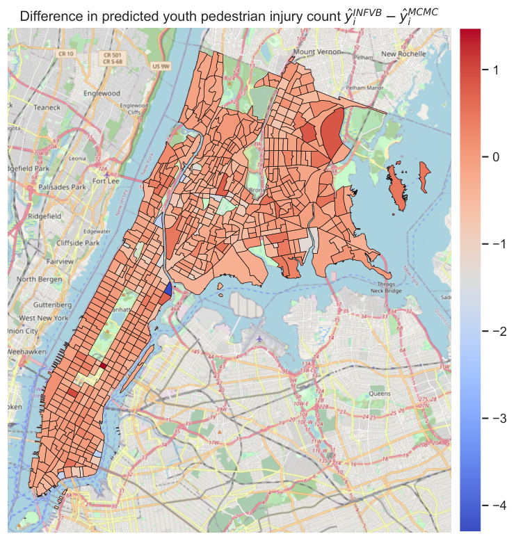
Furthermore, we contrast the in-sample predictive accuracy of the MCMC and INFVB estimators by comparing the predicted injury counts for each census tract. Figure 5 shows histograms of the predicted injury counts for both MCMC and INFVB. It can be seen that the two distributions overlap closely with each other. In addition, Figure 6 visualises the difference between the youth pedestrian injury counts predicted by INFVB () and the corresponding MCMC prediction () for all census tracts. The differences in predicted youth pedestrian injury counts are generally small relative to the observed injury counts (see Figure 2).
Finally, Figure 7 shows histograms of the posterior means of the spatial errors for MCMC and INFVB. The figure suggests that MCMC and INFVB perform equally well at recovering the unobserved spatial dependence.
6 Conclusion
In this paper, we propose and empirically validate a variational Bayes (VB) method for posterior inference in a negative binomial model with unobserved spatial heterogeneity and dependence. The proposed VB method relies on Pólya-Gamma data augmentation to deal with the non-conjugacy of the negative binomial likelihood and an integrated non-factorised specification of the variational distribution to capture posterior dependencies. We benchmark the proposed VB method against MCMC using simulated data as well as real data on youth pedestrian injury counts in the census tracts of the New York City boroughs Bronx and Manhattan. In both applications, the VB approach is around 45 to 50 times faster than MCMC on a regular eight-core processor and emulates the estimation and predictive accuracy of MCMC. The marginal posterior approximations inferred by the VB approach and MCMC also resemble each other closely. The sequential and conditional nature of Gibbs sampling precludes improvement in computational efficiency through parallelisation. By contrast, INFVB can be further accelerated by a factor of up to 20 by taking full advantage of its embarrassingly parallel nature. Thus, INFVB is a scalable alternative to MCMC for the estimation of spatial count data models.
There are several ways in which future work can extend the research presented in the current paper. First, MCMC and VB should be compared on other data sets from other disciplines to collect additional evidence about the relative advantages of the two methods. A second directions for future work is to adapt the proposed VB approach to models with spatio-temporal dependencies. Finally, recent advances in stochastic optimisation could be leveraged to enable the application of the proposed VB method to online inference problems (Hoffman et al., 2013). Online estimation updates parameters continually, as new data points arrive, and thus facilitates the processing of very large data sets and data streams.
Acknowledgements
We would like to thank the associate editor and two anonymous reviewers for their critical assessment of our work. Furthermore, we are grateful to Michel Bierlaire for his helpful comments and suggestions.
Author contribution statement
PB: conception and design, method derivation, manuscript writing and editing. RK: conception and design, method implementation, data preparation and analysis, manuscript writing and editing. DJG: resources, manuscript editing.
References
- Abramowitz and Stegun, (1948) Abramowitz, M. and Stegun, I. A. (1948). Handbook of mathematical functions with formulas, graphs, and mathematical tables, volume 55. US Government printing office.
- Acs et al., (2002) Acs, Z. J., Anselin, L., and Varga, A. (2002). Patents and innovation counts as measures of regional production of new knowledge. Research policy, 31(7):1069–1085.
- Al-Mohy and Higham, (2010) Al-Mohy, A. H. and Higham, N. J. (2010). A new scaling and squaring algorithm for the matrix exponential. SIAM Journal on Matrix Analysis and Applications, 31(3):970–989.
- Anselin, (2013) Anselin, L. (2013). Spatial econometrics: methods and models, volume 4. Springer Science & Business Media.
- Banerjee et al., (2014) Banerjee, S., Carlin, B. P., and Gelfand, A. E. (2014). Hierarchical modeling and analysis for spatial data. CRC press.
- Bansal et al., (2020) Bansal, P., Krueger, R., Bierlaire, M., Daziano, R. A., and Rashidi, T. H. (2020). Bayesian estimation of mixed multinomial logit models: Advances and simulation-based evaluations. Transportation Research Part B: Methodological, 131:124–142.
- Besag, (1974) Besag, J. (1974). Spatial interaction and the statistical analysis of lattice systems. Journal of the Royal Statistical Society: Series B (Methodological), 36(2):192–225.
- Bivand et al., (2014) Bivand, R. S., Gómez-Rubio, V., and Rue, H. (2014). Approximate bayesian inference for spatial econometrics models. Spatial Statistics, 9:146–165.
- Blei et al., (2017) Blei, D. M., Kucukelbir, A., and McAuliffe, J. D. (2017). Variational inference: A review for statisticians. Journal of the American statistical Association, 112(518):859–877.
- Braun and McAuliffe, (2010) Braun, M. and McAuliffe, J. (2010). Variational inference for large-scale models of discrete choice. Journal of the American Statistical Association, 105(489):324–335.
- Castro et al., (2012) Castro, M., Paleti, R., and Bhat, C. R. (2012). A latent variable representation of count data models to accommodate spatial and temporal dependence: Application to predicting crash frequency at intersections. Transportation research part B: methodological, 46(1):253–272.
- Dawid and Sebastiani, (1999) Dawid, A. P. and Sebastiani, P. (1999). Coherent dispersion criteria for optimal experimental design. Annals of Statistics, pages 65–81.
- Dormann, (2007) Dormann, C. F. (2007). Effects of incorporating spatial autocorrelation into the analysis of species distribution data. Global ecology and biogeography, 16(2):129–138.
- Dormann et al., (2007) Dormann, C. F., McPherson, J. M., Araújo, M. B., Bivand, R., Bolliger, J., Carl, G., Davies, R. G., Hirzel, A., Jetz, W., Kissling, D. W., Kühn, I., Ohlemüller, R., Peres-Neto, P. R., Reineking, B., Schröder, B., Schurr, F. M., and Wilson, R. (2007). Methods to account for spatial autocorrelation in the analysis of species distributional data: a review. Ecography, 30(5):609–628.
- Durante et al., (2019) Durante, D., Rigon, T., et al. (2019). Conditionally conjugate mean-field variational bayes for logistic models. Statistical Science, 34(3):472–485.
- Gelman et al., (1992) Gelman, A., Rubin, D. B., et al. (1992). Inference from iterative simulation using multiple sequences. Statistical science, 7(4):457–472.
- Giordano et al., (2018) Giordano, R., Broderick, T., and Jordan, M. I. (2018). Covariances, robustness and variational bayes. The Journal of Machine Learning Research, 19(1):1981–2029.
- Glaser, (2017) Glaser, S. (2017). A review of spatial econometric models for count data. Technical report, Hohenheim Discussion Papers in Business, Economics and Social Sciences.
- Gneiting and Raftery, (2007) Gneiting, T. and Raftery, A. E. (2007). Strictly proper scoring rules, prediction, and estimation. Journal of the American statistical Association, 102(477):359–378.
- Haining and Li, (2020) Haining, R. P. and Li, G. (2020). Regression Modelling Wih Spatial and Spatial-Temporal Data: A Bayesian Approach. CRC Press.
- Han et al., (2013) Han, S., Liao, X., and Carin, L. (2013). Integrated non-factorized variational inference. In Advances in Neural Information Processing Systems, pages 2481–2489.
- Hoffman et al., (2013) Hoffman, M. D., Blei, D. M., Wang, C., and Paisley, J. (2013). Stochastic variational inference. The Journal of Machine Learning Research, 14(1):1303–1347.
- Huang et al., (2013) Huang, A., Wand, M. P., et al. (2013). Simple marginally noninformative prior distributions for covariance matrices. Bayesian Analysis, 8(2):439–452.
- Jordan et al., (2019) Jordan, A., Krüger, F., and Lerch, S. (2019). Evaluating probabilistic forecasts with scoringrules. Journal of Statistical Software, 90(1):1–37.
- Jordan et al., (1999) Jordan, M. I., Ghahramani, Z., Jaakkola, T. S., and Saul, L. K. (1999). An introduction to variational methods for graphical models. Machine learning, 37(2):183–233.
- Kabisa et al., (2016) Kabisa, S., Dunson, D. B., and Morris, J. S. (2016). Online variational bayes inference for high-dimensional correlated data. Journal of Computational and Graphical Statistics, 25(2):426–444.
- Klami, (2015) Klami, A. (2015). Polya-gamma augmentations for factor models. In Asian Conference on Machine Learning, pages 112–128.
- Knowles and Minka, (2011) Knowles, D. A. and Minka, T. (2011). Non-conjugate variational message passing for multinomial and binary regression. In Advances in Neural Information Processing Systems, pages 1701–1709.
- LeSage and Pace, (2007) LeSage, J. P. and Pace, R. K. (2007). A matrix exponential spatial specification. Journal of Econometrics, 140(1):190–214.
- (30) Linderman, S., Adams, R. P., and Pillow, J. W. (2016a). Bayesian latent structure discovery from multi-neuron recordings. In Advances in neural information processing systems, pages 2002–2010.
- Linderman et al., (2015) Linderman, S., Johnson, M. J., and Adams, R. P. (2015). Dependent multinomial models made easy: Stick-breaking with the pólya-gamma augmentation. In Advances in Neural Information Processing Systems, pages 3456–3464.
- (32) Linderman, S. W., Miller, A. C., Adams, R. P., Blei, D. M., Paninski, L., and Johnson, M. J. (2016b). Recurrent switching linear dynamical systems. arXiv preprint arXiv:1610.08466.
- Luts et al., (2015) Luts, J., Wand, M. P., et al. (2015). Variational inference for count response semiparametric regression. Bayesian Analysis, 10(4):991–1023.
- Mannering et al., (2016) Mannering, F. L., Shankar, V., and Bhat, C. R. (2016). Unobserved heterogeneity and the statistical analysis of highway accident data. Analytic methods in accident research, 11:1–16.
- Marshall, (1991) Marshall, R. J. (1991). A review of methods for the statistical analysis of spatial patterns of disease. Journal of the Royal Statistical Society: Series A (Statistics in Society), 154(3):421–441.
- Matheson and Winkler, (1976) Matheson, J. E. and Winkler, R. L. (1976). Scoring rules for continuous probability distributions. Management science, 22(10):1087–1096.
- Morris et al., (2019) Morris, M., Wheeler-Martin, K., Simpson, D., Mooney, S. J., Gelman, A., and DiMaggio, C. (2019). Bayesian hierarchical spatial models: Implementing the besag york mollié model in stan. Spatial and spatio-temporal epidemiology, 31:100301.
- Narayanamoorthy et al., (2013) Narayanamoorthy, S., Paleti, R., and Bhat, C. R. (2013). On accommodating spatial dependence in bicycle and pedestrian injury counts by severity level. Transportation research part B: methodological, 55:245–264.
- Ormerod and Wand, (2010) Ormerod, J. T. and Wand, M. P. (2010). Explaining variational approximations. The American Statistician, 64(2):140–153.
- Park et al., (2016) Park, M., Foulds, J., Chaudhuri, K., and Welling, M. (2016). Variational bayes in private settings (vips). arXiv preprint arXiv:1611.00340.
- Polson et al., (2013) Polson, N. G., Scott, J. G., and Windle, J. (2013). Bayesian inference for logistic models using pólya–gamma latent variables. Journal of the American statistical Association, 108(504):1339–1349.
- Ren et al., (2011) Ren, Q., Banerjee, S., Finley, A. O., and Hodges, J. S. (2011). Variational bayesian methods for spatial data analysis. Computational statistics & data analysis, 55(12):3197–3217.
- Rey and Anselin, (2010) Rey, S. J. and Anselin, L. (2010). Pysal: A python library of spatial analytical methods. In Handbook of applied spatial analysis, pages 175–193. Springer.
- Roberts et al., (1997) Roberts, G. O., Gelman, A., Gilks, W. R., et al. (1997). Weak convergence and optimal scaling of random walk metropolis algorithms. The annals of applied probability, 7(1):110–120.
- Rossi et al., (2012) Rossi, P. E., Allenby, G. M., and McCulloch, R. (2012). Bayesian statistics and marketing. John Wiley & Sons.
- Salimans et al., (2013) Salimans, T., Knowles, D. A., et al. (2013). Fixed-form variational posterior approximation through stochastic linear regression. Bayesian Analysis, 8(4):837–882.
- Simões and Natário, (2016) Simões, P. and Natário, I. (2016). Spatial econometric approaches for count data: An overview and new directions. International Journal of Economics and Management Engineering, 10(1):348–357.
- Strauss et al., (2017) Strauss, M. E., Mezzetti, M., and Leorato, S. (2017). Is a matrix exponential specification suitable for the modeling of spatial correlation structures? Spatial statistics, 20:221–243.
- Tan et al., (2013) Tan, L. S., Nott, D. J., et al. (2013). Variational inference for generalized linear mixed models using partially noncentered parametrizations. Statistical Science, 28(2):168–188.
- (50) US Census Bureau (n.d.). 2012–2016 American Community Survey 5-year estimates.
- Ver Hoef et al., (2018) Ver Hoef, J. M., Peterson, E. E., Hooten, M. B., Hanks, E. M., and Fortin, M.-J. (2018). Spatial autoregressive models for statistical inference from ecological data. Ecological Monographs, 88(1):36–59.
- Wakefield, (2007) Wakefield, J. (2007). Disease mapping and spatial regression with count data. Biostatistics, 8(2):158–183.
- Wang and Blei, (2013) Wang, C. and Blei, D. M. (2013). Variational inference in nonconjugate models. Journal of Machine Learning Research, 14(Apr):1005–1031.
- Wei and Held, (2014) Wei, W. and Held, L. (2014). Calibration tests for count data. Test, 23(4):787–805.
- Wenzel et al., (2019) Wenzel, F., Galy-Fajou, T., Donner, C., Kloft, M., and Opper, M. (2019). Efficient gaussian process classification using pòlya-gamma data augmentation. In Proceedings of the AAAI Conference on Artificial Intelligence, volume 33, pages 5417–5424.
- Whittle, (1954) Whittle, P. (1954). On stationary processes in the plane. Biometrika, pages 434–449.
- Windle et al., (2014) Windle, J., Polson, N. G., and Scott, J. G. (2014). Sampling pólya-gamma random variates: alternate and approximate techniques. arXiv preprint arXiv:1405.0506.
- Wu, (2018) Wu, G. (2018). Fast and scalable variational bayes estimation of spatial econometric models for gaussian data. Spatial statistics, 24:32–53.
- Zhou et al., (2012) Zhou, M., Li, L., Dunson, D., and Carin, L. (2012). Lognormal and gamma mixed negative binomial regression. In Proceedings of the International Conference on Machine Learning. International Conference on Machine Learning, volume 2012, page 1343. NIH Public Access.
Appendix A Conditional posterior update of in MCMC
To obtain the conditional posterior distribution of the dispersion parameter in MCMC, we follow the strategy adopted by Zhou et al., 2012. We represent the negative-binomial-distributed count variable as follows:
Thus, the conditional posterior update of is:
| (29) |
Since the posterior update of is conditional on , we also update the conditional posterior of using the following equation:
| (30) |
Appendix B Supplementary material for INFVB
B.1 Important expressions and identities
where is a digamma function. and are obtained using Gauss-Hermite quadrature (Abramowitz and Stegun, 1948).
B.2 Important expressions to update
| (31) |
Thus, the conditional ELBO of INFVB for the spatial negative binomial model is obtained by inserting expressions presented in equation 31 in the following equation:
| (32) |
The optimal conditional distribution of is obtained by maximising the conditional ELBO or equivalently minimising its negative at each grid point (as detailed in equation 20):
| (33) |