Coverage of an Environment Using
Energy-Constrained Unmanned Aerial Vehicles
Abstract
We study the problem of covering an environment using an Unmanned Aerial Vehicle (UAV) with limited battery capacity. We consider a scenario where the UAV can land on an Unmanned Ground Vehicle (UGV) and recharge the onboard battery. The UGV can also recharge the UAV while transporting the UAV to the next take-off site. We present an algorithm to solve a new variant of the area coverage problem that takes into account this symbiotic UAV and UGV system. The input consists of a set of boustrophedon cells — rectangular strips whose width is equal to the field-of-view of the sensor on the UAV. The goal is to find a coordinated strategy for the UAV and UGV that visits and covers all cells in minimum time, while optimally finding how much to recharge, where to recharge, and when to recharge the battery. This includes flight time for visiting and covering all cells, recharging time, as well as the take-off and landing times. We show how to reduce this problem to a known NP-hard problem, Generalized Traveling Salesperson Problem (GTSP). Given an optimal GTSP solver, our approach finds the optimal coverage paths for the UAV and UGV. Our formulation models multi-rotor UAVs as well as hybrid UAVs that can operate in fixed-wing and Vertical Take-off and Landing modes. We evaluate our algorithm through simulations and proof-of-concept experiments.
Note to Practitioners
There are many applications, such as environmental monitoring, where Unmanned Aerial Vehicles (UAVs) can automate data collection by covering the environment using a mobile sensor. If the environment is large, then it may be infeasible to cover it with an energy-constrained UAV. An option would be to replace the batteries of the UAV along the flight or use a recharging station to aid complete coverage. These alternatives can be limited since they may require manual intervention or inefficient flights back-and-forth between the charging stations. Instead, we present a new approach that uses an Unmanned Ground Vehicle (UGV) as a mobile recharging station. We allow for the UAV wants to autonomously rendezvous with the UGV, land on it, recharge, and potentially be transported to another location before taking-off. The environment to be monitored is given as input in the form of a set of rectangular strips that need to be covered in minimum time with one or more recharging stops. We present an algorithm to find the optimal solution to this problem and verify the performance through simulations.
I Introduction
There are many applications such as infrastructure inspection and environmental monitoring [1, 2, 3], surveillance [4], precision agriculture [5, 6], and search and rescue [7, 8] where Unmanned Aerial Vehicles (UAVs) can be used as mobile, adaptive sensors. A specific use-case in such applications is to provide visual aerial coverage with UAVs. The key challenge we address in this paper is how to cover large environments with an energy-constrained UAV. Particularly, we are interested in scenarios where the coverage is expected to take longer than the battery runtime of the UAV.
One way of addressing energy constraints is by choosing a better platform. Multi-rotor UAVs have limited battery runtime, typically less than 30 minutes [9]. As a result, surveying large areas with a single vehicle may require frequent stops to recharge or replace batteries. Fixed-wing UAVs have longer runtimes, typically less than 90 minutes, but cannot take-off and land vertically or hover in place. The latter characteristic may be essential for visual coverage. Fixed-wing UAVs also have the steering constraints that limit their maneuverability. Hybrid UAVs seek to achieve the best of both worlds — higher maneuverability of a multi-rotor and longer endurance of a fixed-wing. Such hybrid UAVs are commercially available for coverage applications such as precision agriculture [10], environmental monitoring [11] reconnaissance [12] that involve visual coverage of large areas.
While fixed-wing and hybrid UAVs can mitigate some of the energy limitations, there may still be environments that are too large or need persistent monitoring beyond the runtime of the UAV. To address this inherit limitation, we propose a solution that uses Unmanned Ground Vehicles (UGVs) as mobile recharging stations. In our prior work [13], we presented an approach to visit a set of specified points of interest using a multi-rotor UAV with a UGV acting as a mobile recharging station. In this paper, we investigate the coverage problem using hybrid UAVs.
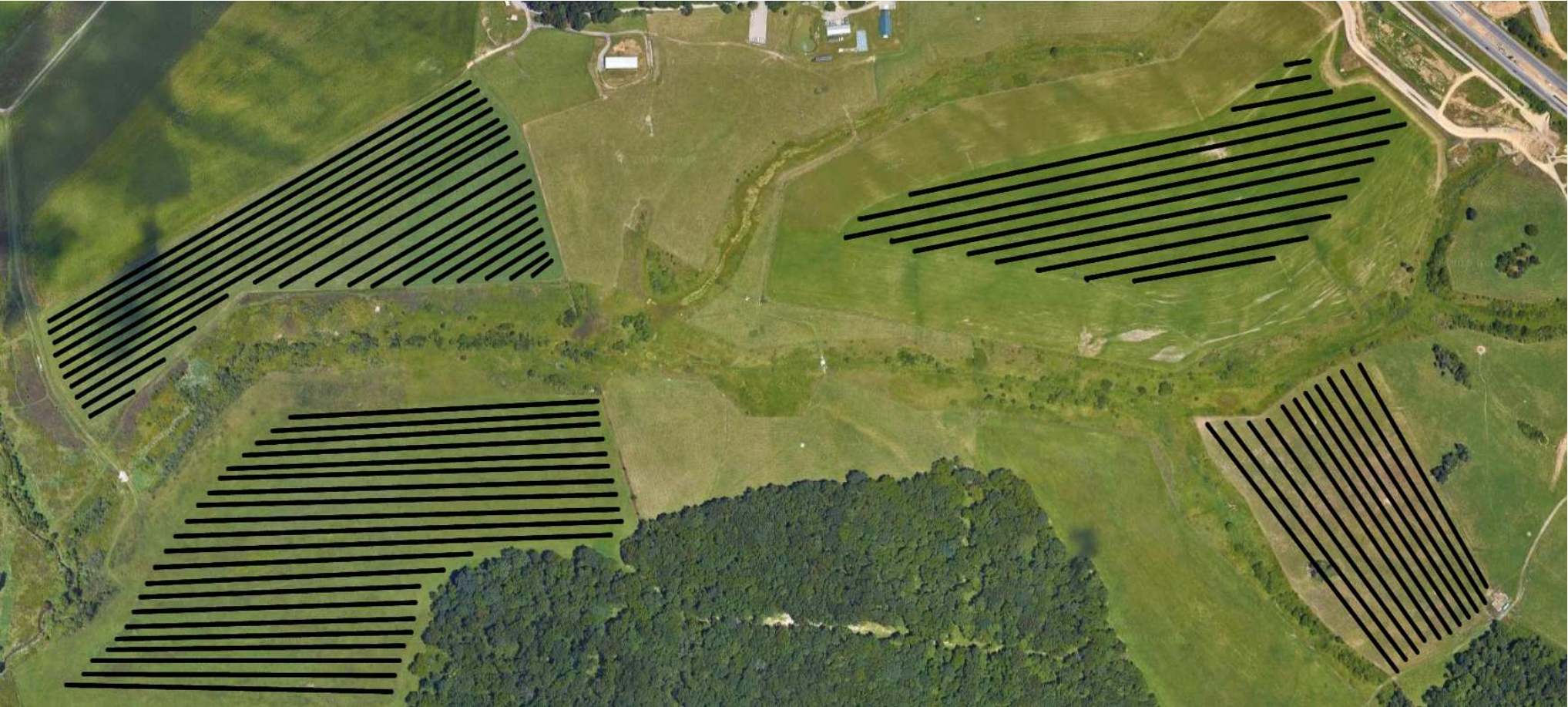
The input to our planner is a set of boustrophedon cells — rectangular regions whose width is equal to the footprint of the UAV’s sensor. The boustrophedon cells can be obtained by decomposing regions that need to be covered [14, 15]. Figure 1 shows a motivating example of surveying crops in four fields. Here, each boustrophedon cells corresponds to a row of crops that need to be imaged by the UAV.
A boustrophedon cell can be covered by the UAV entering from either end and exiting from the other — the planner must find the optimal sequence in which to cover the boustrophedon cells as well as the corresponding entry and exit sites for each boustrophedon cells.
We consider scenarios where the UAV can land on the UGV and either recharge in-place or recharge while the UGV transports the UAV to the next take-off site. We present an algorithm that plans a tour for the UAV and a path for the UGV, such that the UAV can cover an area in the minimum time while never running out of charge. This includes not only the flight time of the UAV but also the time it takes to recharge as well as the taking-off and landing times. The output tour given by our planner specifies not only the order in which to cover the boustrophedon cells but also the charging schedule and flight mode that the UAV will be in. In particular, the planner outputs where and how to recharge the battery, how much to recharge by, and whether to fly in multi-rotor flight mode or fixed-wing flight mode.
This problem is a generalization of the NP-hard Traveling Salesperson Problem (TSP) [16]. Our solution is based on reducing the coverage problem to the Generalized TSP (GTSP) [17]. Specifically, we present an algorithm that is guaranteed to find the optimal coverage tour for the UAV, as long the GTSP solver produces optimal tours. While no polynomial-time optimal algorithms are believed to exist for NP-hard problems, there are solvers that find optimal solutions to many instances in reasonable amounts of time in practice. We use one such solver, Generalized Large Neighborhood Search (GLNS) [18], that finds optimal solutions for GTSP instances. We empirically evaluate the performance of our algorithm using the GLNS solver.
This work extends our prior work [13] wherein we presented a method to visit a set of points, instead of regions, using a multi-rotor. This journal article extends the preliminary work presented in [19] wherein we presented a method to visit a set of boustrophedon cells using a multi-rotor UAV and UGV as a mobile recharging station. In this paper, we extend the results to account for a hybrid UAV. Hybrid UAVs add the challenges of handling multiple modes of flight, Dubins’ steering constraints when executing fixed-wing flight, and the different energy discharge rates dependent on the flight mode.
II Related Work
Environmental coverage is a well-studied problem in robotics [20, 21]. The variant most closely related to the one we study is that of decomposing a known environment into various cells and then finding a route to sweep (i.e., cover) each cell [22, 23, 24, 25, 26]. In this work, we assume that the first step (cell decomposition) has been solved and focus on the problem of routing the UAV to cover the cells in minimal time, while keeping track of the battery level and flight mode. We introduce a novel means of environmental coverage using a hybrid UAV system, which can leverage aspects of a multi-rotor UAV, such as vertical take-off and landing, and fixed-wing UAV, such as long flight times. Specifically, we take as input a boustrophedon cell decomposition which can be found using techniques given by [15].
A number of algorithms have also been developed for the second step, i.e., routing to cover all cells, under various constraints. In particular, Karapetyan et al. presented a multi-robot coverage algorithm for boustrophedon cell decomposition for point robots [27]. Yu et al. presented a coverage algorithm for a single robot with Dubins steering constraints [28]. Lewis et al. later proved that problem NP-hard, and showed how to reduce the graph to obtain practical solutions [29]. Bochkarev and Smith present a method for decomposing an environment to minimize the number of turns needed to cover an area, but do not consider energy-limited robots and consequently, do not need to keep track of the battery level of the robot [26]. Most recently, Karapetyan et al. presented two techniques to cover a collection of cells with multiple Dubins vehicles [30].
The underlying ideas in the aforementioned works are similar — reduce the problem of covering all cells to a variant of the TSP, solve the TSP, and convert the resulting solution back to a tour for the robots. Our approach extends these ideas for the case of a robot with limited energy capacity which can be recharged along the way and a robot with multiple flight modes, taking advantage of both multi-rotor and fixed-wing modalities. This requires us to keep track of energy level of the robot along the tour and the flight modes, which further complicates the problem. Nevertheless, we show that by reducing it to GTSP, we can obtain optimal solutions in reasonable amounts of time.
Many other works also analyze the coverage problem using fixed-wing UAVs, but do not have the advantages of a hybrid system. Paull et al. considered area coverage using onboard sensors for a fixed-wing UAV [31]. However the authors take an online approach, leading to solutions that are sub-optimal for environmental coverage. Xu et al. present an algorithm for optimal terrain coverage using fixed-wing UAV [32]. Their method considers minimizing overlapping areas of coverage, the method in this paper does not allow for any overlapping coverage. Also we provide experiments that utilize charging stations and implement a hybrid system. Coombes et al. use a fixed-wing UAV for survey coverage path planning in windy environments [33]. This approach studies the effects of wind on a fixed-wing system and proposes algorithms that solve for paths that take into account the wind patterns of the environment.
There have been algorithms for assigning and routing with one or more stationary recharging stations [34, 35, 36]. Kim et al. present a Mixed Integer Linear Programming approach for assigning UAVs to stationary recharging stations while taking into account the task objective [34]. Liu and Michael presented a method for assigning UAVs to UGVs acting as recharging stations [36].
In our previous work [6, 13, 19], we studied the problem of visiting a set of boustrophedon cells (rectangles with the width of the field-of-view (FOV) of the sensor in a 2D plane) using an energy-limited UAV with only one mode of flight. In [6], we showed how to maximize the number of sites visited in a single charge when the UAV is allowed to land on the UGV and let the UGV transport it to the next take-off site without the UAV expending energy. In [13], we extended this to also allow for the UGV to recharge the UAV either while stationary or while being transported to the next deployment site. In [19], we further extend the work from [13] to conduct coverage of boustrophedon cells. This paper extends the prior work from merely having a single mode of flight to having multiple modes of flight. As a result, the planner must decide not only the order in which the boustrophedon cells should be visited but also the directions in which to cover them and what is the optimal flight mode to use.
III Problem Formulation
The input to our algorithm is a set of boustrophedon cells that need to be covered by the UAV. A boustrophedon cell is a rectangular strip whose width is equal to the diameter of the FOV of the sensor onboard the robot. An example is shown in Figure 2 and a larger example is shown in Figure 1.
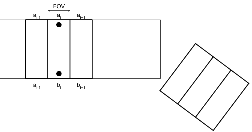
Each boustrophedon cell is described by two sites, and , where is the index of the boustrophedon cell. These sites are placed at two ends of the rectangular strip. A boustrophedon cell is said to be covered if the UAV travels in a straight line from to or from to . The UAV can enter a boustrophedon cell from either site, or . However, once the UAV has entered a boustrophedon cell it is required to cover the entire boustrophedon cell and exit from the other site. The coverage algorithm must choose one of the sites as the entry site as well as how to traverse the boustrophedon cell. We slightly generalize the traditional notion of a boustrophedon cell by allowing them to be oriented in different directions. That is, we do not require the boustrophedon cells to be parallel to each other.
We make the following assumptions:
- •
the UAV has an initial battery charge of ;
- •
the UAV flies at a fixed-altitude plane when covering a boustrophedon cell;
- •
the UAV travels at unit speed in multi-rotor mode;
- •
the UGV has unlimited fuel/battery capacity;
- •
edges can only conduct recharging if they correspond with sites the UGV can visit.
We use and to represent the time taken by the UAV to take-off from the UGV to reach the fixed-altitude plane and land from this plane onto the UGV, respectively. represents the total distance a UAV can travel with 100% battery capacity in multi-rotor mode.11 1 Strictly speaking, we maintain a reserve battery capacity to take-off from ground to reach the fixed altitude plane and land from the fixed-altitude plane on the ground. In this paper, when we refer to 100% battery capacity, it excludes this reserve battery for taking-off and landing. We discretize the battery capacity into levels. represents the rate the battery gets recharged per unit time. represents the ratio of multi-rotor to fixed-wing battery consumption. This is above if the fixed-wing consumes less battery than the multi-rotor over a fixed distance. We define the turn radius of the fixed-wing as . When our UAV is in fixed-wing mode it will obey the constraints of a Dubins vehicle.
Let denote the site chosen by a coverage algorithm to be the entry site of the boustrophedon cell in the order in which they are to be visited. Correspondingly, denotes the site chosen to be the exit site of the boustrophedon cell, i.e., . denotes the order in which the boustrophedon cells are to be visited. That is, gives the boustrophedon cell that is visited.
We use , , and to denote , , and , respectively. We denote by the time it takes for the UGV to travel along the ground from the exit site of boustrophedon cell to the entry site of the next visited boustrophedon cell. We use to represent the time it takes for the UAV to travel in multi-rotor mode from the exit site of the boustrophedon cell to the entry site of the next boustrophedon cell visited. Similarly, gives the time taken by the UAV in multi-rotor mode to cover the boustrophedon cell. We use to represent the time it takes for the UAV to travel in fixed-wing mode from the exit site of the boustrophedon cell to the entry site of the next boustrophedon cell visited. Similarly, gives the time taken by the UAV in fixed-wing mode to cover the boustrophedon cell.
Suppose is a path that visits every boustrophedon cell in the order given by and with entry and exit sites given by . The cost of the path depends on how the UAV travels between consecutive boustrophedon cells. Consider traveling from to and then on to along . We have the following components for this part of the path:
- •
The UAV must fly from to . The time taken is given by or . Let be an indicator function that denotes whether the UAV chooses to fly in multi-rotor or fixed-wing mode.
- •
It can then choose to land on the UGV at , recharge in-place, and take-off to reach the fixed-altitude plane at . Let be an indicator function that denotes whether the UAV chooses to do this or not.
- •
It can then choose to either fly from to or land on the UGV at , recharge while being carried by the UGV to the next site, then take-off at to reach the fixed-altitude plane. Let be an indicator function denoting whether the UAV travels with the UGV or not. Note that if UAV chooses flight then the indicator function is also used to denote true for multi-rotor or false for fixed-wing flight.
- •
It can then choose to land on the UGV at , recharge in-place, and take-off to reach the fixed-altitude plane at . Let be an indicator function that denotes whether the UAV chooses to do this or not.
Based on these choices, the cost of traveling from to is given by:
| (1) |
Here, is a function which gives the amount by which the battery should be recharged between two sites.
Therefore, we can define the cost of the path as:
| (2) |
At the end of we take the minimum of and because at the last site the UAV will not need to conduct any type of charging and therefore will only need to cover the site. We are now ready to define the problem.
Problem 1 (Multiple Polygon Coverage)
Given a set of boustrophedon cells to be covered, find a path , which contains , , , , and , for the UAV that visits and covers all of the boustrophedon cells, while minimizing the cost (Equation 2), and ensuring that the UAV does not run out of battery capacity. The path must specify the order in which to visit the boustrophedon cells, , the entry site for each boustrophedon cell, , the recharging indicator functions, , and , the amount of recharging at a site, , and when to change flight modes during coverage.
Note that finding a path for the UAV necessitates finding a path for the UGV that supports the UAV recharging schedule.
IV GTSP-based Algorithm
We solve the polygon coverage problem by reducing it to GTSP. In this section, we describe in detail the reduction to GTSP. The input to GTSP is a directed weighted graph where the vertices are partitioned into clusters. The objective is to find a minimum cost tour that visits exactly one vertex in each cluster. If all the clusters contain exactly one vertex, then GTSP trivially reduces to TSP. We show how to create the clusters, the edges between the clusters and then show how to convert the solution for GTSP into tours for the UAV and the UGV.
IV-A Vertices and Clusters
We discretize the battery’s charge states into levels. We create vertices, one corresponding to each discretized battery level, for each site and corresponding to boustrophedon cell . The vertex is denoted by or , where corresponds to the discretized battery level. Thus there are total vertices in the graph. We create one cluster per boustrophedon cell. This cluster contains vertices, of them corresponding to and of them corresponding to .
IV-B Edges
We create an edge between every pair of vertices that do not belong to the same cluster (i.e., do not belong to the same boustrophedon cell). Recall that a vertex corresponds to the entry site for the corresponding boustrophedon cell. Therefore, an edge between two vertices represents the UAV starting at the entry site of the first boustrophedon cell and ending at the entry site of the next boustrophedon cell. This includes two travel legs: coverage of the first boustrophedon cell and then traveling from the exit site of the first boustrophedon cell towards the second boustrophedon cell. Recall that the UAV must always fly the first leg, either in multi-rotor or fixed-wing mode; however, the second leg can be a combination of recharging, flying, and/or recharging while traveling on the UGV.
Equation 1 gives the cost of traveling between two entry sites of different boustrophedon cells. The actual cost depends on the five binary indicator variables: , , , , and . This gives a total of possible travel options. However, fourteen of these thirty-two options are redundant. Specifically, if the UAV chooses to recharge while traveling on the UGV, then also recharging on either end of this leg is redundant and, in fact, more time-consuming since it will have to take-off and land more than once. Formally, if , then the optimal algorithm will never set nor . Also if then what and is equal to does not matter and we can eliminate those possibilities as well. We leave two states where and to handle the state in which the UAV will use the UGV as a transport. Therefore, of these possibilities, we can eliminate fourteen, leaving a total of eighteen possibilities. These are shown in Figures 3, 4, 5, 6, 7. Note that since we assume that the UAV starts with 100% battery capacity, we will never recharge at the first entry site.
We denote the eighteen edge combinations using the notation: M = Multi-rotor, F = Fixed-wing, D = Down/Land, U = Up/Take-off, and T = Transit. The first leg is always the UAV flying to cover the boustrophedon cell. We describe the actual edge costs in the remainder of this section.
In the following, we show how to compute the edge cost between vertices and . denotes the battery at if going from and . Note that there will also be edges between and , and , and and . The costs for these edges can be obtained using the same formula just by swapping with and vice-versa.

The cost of the M-M, F-F, M-F, and F-M type of edges, Figure 3, between and is if the energy required to go from to and then to is more than . Else, the edge cost is given by:
| (3) |
| (4) |
| (5) |
| (6) |

The cost of the M-DTU and F-DTU type of edges, Figure 4, between and is equal to if the energy required to go from to is more than . Else, the edge cost is given by:
| (7) |
| (8) |
where gives the recharging amount.

The cost of the M-MDU, F-FDU, M-FDU, and F-MDU type of edges, Figure 5, between and is if the energy required to go from to and then to is more than . Else, the edge cost is:
| (9) |
| (10) |
| (11) |
| (12) |
where gives the recharging amount.

The cost of the M-DUM, F-DUF, M-DUF, and F-DUM type of edges, Figure 6, between and is equal to if the energy required to go from to is more than and then to is more than . Else, the edge cost is given by:
| (13) |
| (14) |
| (15) |
| (16) |
where gives the recharging amount.

The cost of the M-DUMDU, F-DUFDU, M-DUFDU, and F-DUMDU type of edges, Figure 7, between and is equal to if the energy required to go from to is more than and then to is more than . Else, the edge cost is given by:
| (17) |
| (18) |
| (19) |
| (20) |
where and gives the recharging amount for and , respectively.
The actual edge cost between and is the minimum of all eighteen types. Specifically, the final edge cost is given by:
| (21) |
We also keep track of which type of edge gives the final edge cost. This is used when converting the GTSP tour into a solution for the original problem.
IV-C Solving GTSP
We solve the GTSP instance using the GLNS solver [18]. GLNS uses a neighborhood search heuristic to find the optimal solution for the given GTSP instance. GLNS also allows for finding feasible solutions in lesser time, potentially at the expense of optimality.
Common alternatives for finding the optimal GTSP solution are Integer Programming or reducing GTSP to TSP [17] and then using a TSP solver such as Concorde [37]. In our previous work [13], we showed that GLNS finds the optimal solution for a similar class of GTSP instances in times that are at least an order of magnitude faster than the other approaches. As a result, we focus on only using GLNS for solving the GTSP instances in this paper.
IV-D Converting the GTSP solution to a Coverage Tour
The optimal tour obtained from the GTSP solver is a tour that visits exactly one vertex in each cluster. Recall that one cluster corresponds to one boustrophedon cell. The optimal tour will visit only one vertex within a cluster. The chosen vertex corresponds specifies the entry site for the boustrophedon cell as well as the corresponding battery level.
For example, if the edge between and is selected, then this implies the UAV will cover the boustrophedon cell with as the entry site and as the exit site. Then, the UAV will travel from to the entry site of the next boustrophedon cell which is chosen to be . The actual mode of transportation between and depends on the type of the edge, denoted by the eighteen edges in Figures 3, 4, 5, 6, 7. Depending the type, we construct the actual tour and recharging schedule for the UAV.
We can determine the UGV path based on the type of edges chosen by considering the edges in the order they appear in the optimal GTSP tour. For a M-M, M-F, F-M, F-F edge, the UGV is not required. For an M-DUM, F-DUF, M-DUF, F-DUM edge, we add the exit site of the first boustrophedon cell to the UGV tour. Similarly, for an M-MDU, F-FDU, M-FDU, F-MDU, we add the entry site of the second boustrophedon cell to the UGV tour. Finally, for M-DUMDU, F-DUFDU, M-DUFDU, F-DUMDU, M-DTU, and F-DTU edges, we add the exit site of the first boustrophedon cell and the entry site of the second one to the UGV tour.
IV-E Performance Guarantees
If the GTSP solver finds the optimal tour, then the corresponding UAV tour is also the optimal solution to Problem 1 with the additional assumption that the UGV is as fast as the UAV. If the UAV is faster than the UGV, then it is possible that the solution yields paths where the UAV reaches a landing site before the UGV. In such cases, one possibility is to have more than one UGV that can support the UAV tour. In our previous work [38], we presented an Integer Programming solution that minimizes the number of slower UGVs required to support the UAV tour.
V Simulations
In this section, we present qualitative and quantitative results to evaluate the proposed algorithm. In particular, we analyze the effect of various parameters on the tour cost and the computational time of the algorithm. The experiments were run on an Ubuntu 16.04 computer with an Intel i7-8750H CPU running at 2.2GHz, with 6 physical cores, 32GB of RAM, and a GTX 1070 GPU.
V-A Qualitative Examples
We use the boustrophedon cells given in Figure 1 as the input. There are a total of 66 boustrophedon cells. The solution is shown in Figure 8. The boustrophedon cells are marked with rectangles. The input parameters were set to: , , , , , , and . The UGV speed was set to be 20% as that of the UAV.
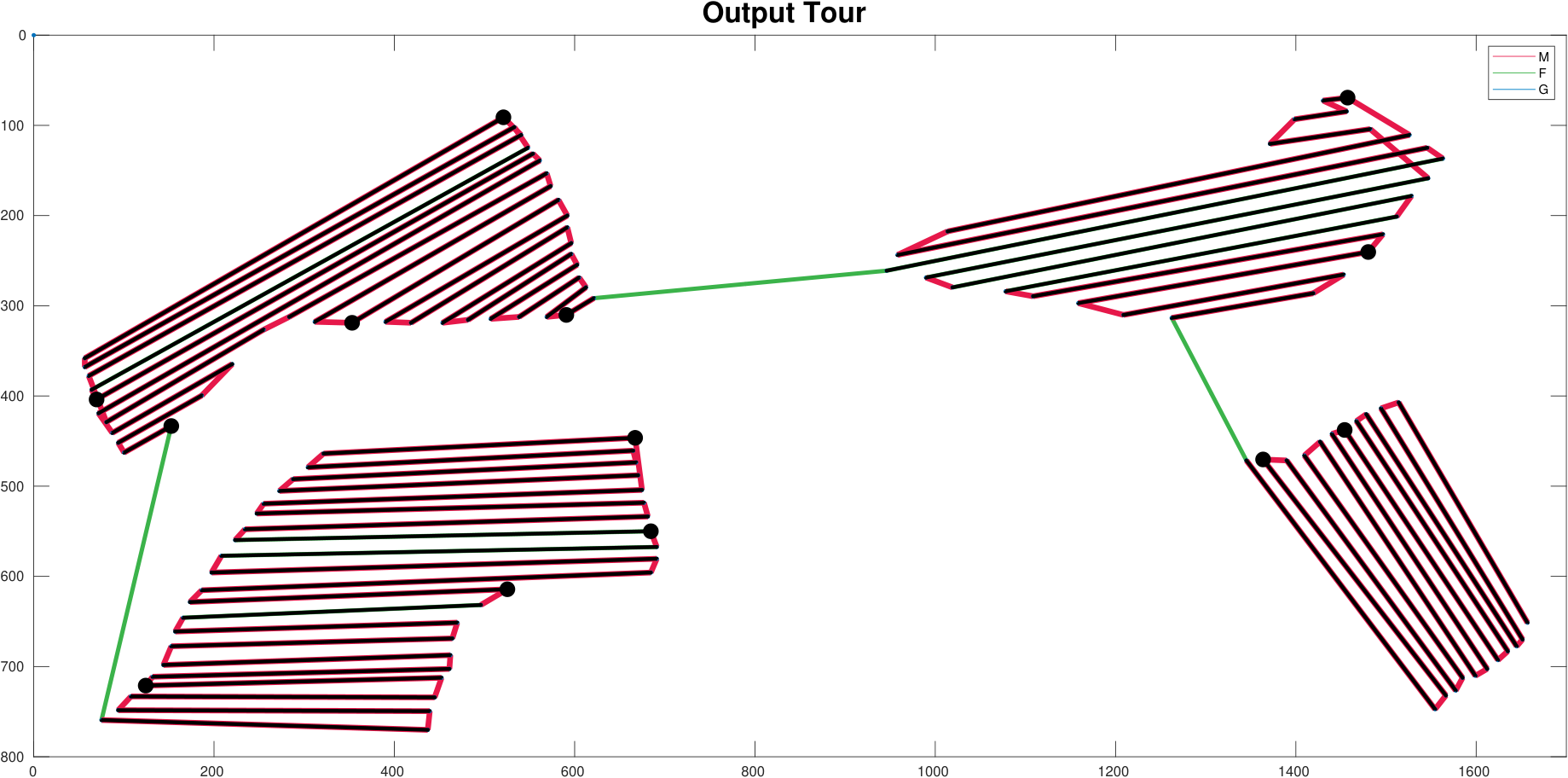


We compare the results of our algorithm with a naive baseline. The baseline approach visits each boustrophedon cell in the same order in which they appear along the boundary of the polygon. The UAV lands to recharge on the UGV only when covering the next boustrophedon cell would deplete it of the remaining energy. Once on the UGV, the UAV recharges to maximum capacity. The baseline approach produces a tour which requires 29564 seconds for completion (as given by Equation 2) where as the proposed algorithm produces a tour which requires 25595 seconds.
Figures 9(b)– 9(g) presents additional qualitative examples that show the effect of changing multiple input parameters on the solution for the input given in Figure 9(a). We observe that if the UAV has enough energy capacity then the final tour does not use the UGV (Figure 9(b) and Figure 9(c)). If the UGV is significantly slower than the UAV and is small, then the UAV only recharges in-place (Figure 9(d), Figure 9(e), and Figure 9(f)) and does not use M-DTU or F-DTU edges. However, if the UGV is not as slow, then the tour will use M-DTU and F-DTU edges (Figure 9(g)). We present quantitative evaluation of these parameters next.
V-B Effect of Changing on the Tour Cost
Next, we study the effect of changing the total battery capacity, i.e., changing , on the total tour time. We randomly generate 15 boustrophedon cells in a 100m 100m environment such that no two boustrophedon cells intersect with each other and each boustrophedon cell is no more than 10 meters long. Figure 10(a) shows one example.
We vary from 10 meters to 50 meters. We use the same set of 15 boustrophedon cells for each value of . Figure 10(b) shows the average, minimum, and maximum value of the optimal tour cost. We observe that the tour cost decreases as increases, as is expected. We also observe a step decrease in the minimum and maximum tour costs as increases. This can be attributed to the fact that as increases the UAV can travel a larger distance without running out of energy. Therefore, it may need to land/take-off fewer number of times. Each landing and taking-off operation costs a fixed amount of time. Therefore, we see a step decrease in the tour cost as increases.
V-C Effect on the Computational Time
Next, we empirically analyze the computational time as a function of some of the input parameters.
Figure 11 shows the effect of increasing the number of input boustrophedon cells on the computational time. The input number of boustrophedon cells is varied from 10 to 50 in steps of 1. The figure shows the average, minimum, and maximum computational times for 10 random instances. The input parameters for these experiments were kept the same: , , , , , and .
Figure 11 shows the effect of increasing the battery level, i.e., , on the computational time. We vary from 10 to 100 in steps of 10. The input parameters for these experiments were: , , , , and . The figure shows the average, minimum, and maximum computational time for 10 random instances with 15 boustrophedon cells each.
We observe that the computational time increases (perhaps, exponentially) with increasing the number of input boustrophedon cells and battery level. Nevertheless, the computational time is still small enough (less than 50 minutes) for moderately sized instances (50 boustrophedon cells).
VI Field Experiments
We conducted proof-of-concept field experiments using the UAV and UGV shown in Figure 12(c). The UAV is a DJI 450 frame [39] with a Pixhawk 2.1 [40] flight controller running the APM firmware [41] and the UGV is a Clearpath Husky [42]. The UAV is equipped with dual GPSs, a downwards facing LIDAR (for relative altitude estimation) and the IR-Lock infrared camera [43]. The UGV is fitted with infrared LED beacons. The IR-Lock system [43] allows for precision landing on the UGV with up to 10cm accuracy in nominal wind conditions. More details on the system are reported in our prior work [38].


Figure 12(a) shows the input boustrophedon cells for the proof-of-concept experiment conducted at Kentland Farms at Virginia Tech. The motion of the UGV is restricted to only those sites that lie on the road. Specifically, we allow edges that conduct recharging to only occur if they correspond with sites are on the road. These sites are marked in red in Figure 12(a). The output tour for the UAV is shown in Figure 12(b). The following parameters were used as input to the outdoor field experiments: , , , , 13 boustrophedon cells, , , and . Since our platform is a multi-rotor, we set . This forces the fixed-wing flights to be more expensive than the multi-rotor ones. With the addition of our algorithm will never use any edges that use the fixed-wing mode.
The GPS trace of the UAV and the UGV are shown in Figures 12(d) and 12(e). Both robots were fully autonomous during the trial that lasted 12 minutes, including taking-off and landing from the ground robot. A video of the trial is submitted as part of the multimedia attachment. The trial provides a proof-of-concept demonstration of the algorithm.
VII Conclusion
We present an algorithm for optimal coverage of boustrophedon cells with an energy-limited UAV and a UGV. The UGV acts as a mobile recharging station that can mule the UAV between sites, while the UAV can switch between multi-rotor and fixed-wing flight modes. We analyze the effects of various input parameters on the total tour cost as well as the computational time. We evaluate our algorithm through field experiments.
If the UGV is slower, it is possible that the UAV may reach a site before the UGV. In [38], we showed how find the minimum number of UGVs required to ensure that the UAV can execute its tour without having to wait for the UGV. A possible extension is to find a tour for a fixed number of slower UGVs that still ensures that the UAV does not need to wait for the UGV. We restrict the UAV to land and take-off only from the entry/exit sites of a boustrophedon cell. A possible extension would be to relax this assumption which can result in even shorter tours.
References
- [1] P. Liu, A. Y. Chen, Y.-N. Huang, J. Han, J. Lai, S. Kang, T. Wu, M. Wen, and M. Tsai, “A review of rotorcraft unmanned aerial vehicle (uav) developments and applications in civil engineering,” Smart Struct. Syst, vol. 13, no. 6, pp. 1065–1094, 2014.
- [2] T. Ozaslan, S. Shen, Y. Mulgaonkar, N. Michael, and V. Kumar, “Inspection of penstocks and featureless tunnel-like environments using micro uavs,” in International Conference on Field and Service Robotics, 2013.
- [3] M. Dunbabin and L. Marques, “Robots for environmental monitoring: Significant advancements and applications,” IEEE Robotics and Automation Magazine, vol. 19, no. 1, pp. 24 –39, Mar 2012.
- [4] N. Michael, E. Stump, and K. Mohta, “Persistent surveillance with a team of mavs,” in Intelligent Robots and Systems (IROS), 2011 IEEE/RSJ International Conference on. IEEE, 2011, pp. 2708–2714.
- [5] J. Das, G. Cross, C. Qu, A. Makineni, P. Tokekar, Y. Mulgaonkar, and V. Kumar, “Devices, systems, and methods for automated monitoring enabling precision agriculture,” in Proceedings of IEEE Conference on Automation Science and Engineering. IEEE, 2015, pp. 462–469.
- [6] P. Tokekar, J. Vander Hook, D. Mulla, and V. Isler, “Sensor planning for a symbiotic UAV and UGV system for precision agriculture,” IEEE Transactions on Robotics, 2016.
- [7] T. Sherman, J. Tellez, T. Cady, J. Herrera, H. Haideri, J. Lopez, M. Caudle, S. Bhandari, and D. Tang, “Cooperative search and rescue using autonomous unmanned aerial vehicles,” in 2018 AIAA Information Systems-AIAA Infotech@ Aerospace. ARC, 2018, p. 1490.
- [8] Y. Sung and P. Tokekar, “Algorithm for searching and tracking an unknown and varying number of mobile targets using a limited fov sensor,” in Robotics and Automation (ICRA), 2017 IEEE International Conference on. IEEE, 2017, pp. 6246–6252.
- [9] J. Flynt, “10 best long flight time drones: Fantastic battery life - 3d insider,” https://3dinsider.com/long-flight-time-drones/, November 2019, (Accessed on 09/21/2018).
- [10] AeroVironment, “Av drone analytics - drones & data analytics with quantix & dss,” https://www.avdroneanalytics.com/, 2020, (Accessed on 05/27/2020).
- [11] Wingtra, “Wingtraone – mapping drone for high-accuracy aerial surveys — wingtra,” https://wingtra.com/mapping-drone-wingtraone/#intro, 2020, (Accessed on 05/27/2020).
- [12] AeroVironment, “Quantix™ recon,” https://www.avinc.com/tuas/quantix-recon, 2020, (Accessed on 05/27/2020).
- [13] K. Yu, A. K. Budhiraja, and P. Tokekar, “Algorithms and experiments on routing of unmanned aerial vehicles with mobile recharging stations,” in Proc. IEEE International Conference on Robotics and Automation. IEEE International Conference on Robotics and Automation, 2018.
- [14] H. Choset and P. Pignon, “Coverage path planning: The boustrophedon decomposition,” in Proceedings of the International Conference on Field and Service Robotics, 1997, pp. 3–91.
- [15] I. Maza and A. Ollero, “Multiple uav cooperative searching operation using polygon area decomposition and efficient coverage algorithms,” in Distributed Autonomous Robotic Systems 6. Springer, 2007, pp. 221–230.
- [16] S. Arora, “Polynomial time approximation schemes for euclidean traveling salesman and other geometric problems,” Journal of the ACM (JACM), vol. 45, no. 5, pp. 753–782, 1998.
- [17] C. E. Noon and J. C. Bean, “An efficient transformation of the generalized traveling salesman problem,” INFOR, vol. 31, no. 1, p. 39, 1993.
- [18] S. L. Smith and F. Imeson, “GLNS: An effective large neighborhood search heuristic for the generalized traveling salesman problem,” Computers & Operations Research, vol. 87, pp. 1–19, 2017.
- [19] K. Yu, J. M. O’Kane, and P. Tokekar, “Coverage of an environment using energy-constrained unmanned aerial vehicles,” in 2019 International Conference on Robotics and Automation (ICRA). IEEE, 2019, pp. 3259–3265.
- [20] H. Choset, “Coverage for robotics - a survey of recent results,” Annals of Mathematics and Artificial Intelligence, vol. 31, pp. 113–126, 2001.
- [21] E. Galceran and M. Carreras, “A survey on coverage path planning for robotics,” Robotics and Autonomous Systems, vol. 61, no. 12, pp. 1258–1276, 2013.
- [22] W. Huang, “Optimal line-sweep-based decompositions for coverage algorithms,” in Proc. the IEEE Int. Conf. on Robotics and Automation, vol. 1, 2001, pp. 27 – 32.
- [23] Z. Yao, “Finding efficient robot path for the complete coverage of a known space,” in Proc. IEEE International Conference on Robotics and Automation, 2006.
- [24] E. Gonzalez, O. Alvarez, Y. Diaz, C. Parra, and C. Bustacara, “BSA: a complete coverage algorithm,” in Proc. IEEE International Conference on Robotics and Automation, 2005.
- [25] Y.-H. Choi, T.-K. Lee, S.-H. Baek, and S.-Y. Oh, “Online complete coverage path planning for mobile robots based on linked spiral paths using constrained inverse distance transform,” in Proc. IEEE/RSJ International Conference on Intelligent Robots and Systems, 2009.
- [26] S. Bochkarev and S. L. Smith, “On minimizing turns in robot coverage path planning,” in Automation Science and Engineering (CASE), 2016 IEEE International Conference on. IEEE, 2016, pp. 1237–1242.
- [27] N. Karapetyan, K. Benson, C. McKinney, P. Taslakian, and I. Rekleitis, “Efficient multi-robot coverage of a known environment,” in Proc. IEEE/RSJ International Conference on Intelligent Robots and Systems, Vancouver, BC, Canada, Sept. 2017.
- [28] X. Yu, T. A. Roppel, and J. Y. Hung, “An optimization approach for planning robotic field coverage,” in Proc. Annual Conference of the IEEE Industrial Electronics Society, 2015.
- [29] J. S. Lewis, W. Edwards, K. Benson, I. Rekleitis, and J. M. O’Kane, “Semi-boustrophedon coverage with a dubins vehicle,” in Proc. IEEE/RSJ International Conference on Intelligent Robots and Systems, 2017.
- [30] N. Karapetyan, J. Moulton, J. S. Lewis, A. Q. Li, J. M. O’Kane, and I. Rekleitis, “Multi-robot dubins coverage with autonomous surface vehicles,” in Proc. IEEE International Conference on Robotics and Automation, 2018.
- [31] L. Paull, C. Thibault, A. Nagaty, M. Seto, and H. Li, “Sensor-driven area coverage for an autonomous fixed-wing unmanned aerial vehicle,” IEEE transactions on cybernetics, vol. 44, no. 9, pp. 1605–1618, 2013.
- [32] A. Xu, C. Viriyasuthee, and I. Rekleitis, “Optimal complete terrain coverage using an unmanned aerial vehicle,” in 2011 IEEE International conference on robotics and automation. IEEE, 2011, pp. 2513–2519.
- [33] M. Coombes, W.-H. Chen, and C. Liu, “Fixed wing uav survey coverage path planning in wind for improving existing ground control station software,” in 2018 37th Chinese Control Conference (CCC). IEEE, 2018, pp. 9820–9825.
- [34] J. Kim, B. D. Song, and J. R. Morrison, “On the scheduling of systems of uavs and fuel service stations for long-term mission fulfillment,” Journal of Intelligent & Robotic Systems, pp. 1–13, 2013.
- [35] S. Ahmed, A. Mohamed, K. Harras, M. Kholief, and S. Mesbah, “Energy efficient path planning techniques for uav-based systems with space discretization,” in Wireless Communications and Networking Conference (WCNC), 2016 IEEE. IEEE, 2016, pp. 1–6.
- [36] L. Liu and N. Michael, “Energy-aware aerial vehicle deployment via bipartite graph matching,” in Unmanned Aircraft Systems (ICUAS), 2014 International Conference on. IEEE, 2014, pp. 189–194.
- [37] D. Applegate, R. Bixby, V. Chvatal, and W. Cook, “Concorde tsp solver,” URL http://www. tsp. gatech. edu/concorde, 2006.
- [38] K. Yu, A. K. Budhiraja, S. Buebel, and P. Tokekar, “Algorithms and experiments on routing of unmanned aerial vehicles with mobile recharging stations,” Journal of Field Robotics, vol. 36, no. 3, pp. 602–616, 2019.
- [39] Amazon, “Amazon.com: Dji flame wheel f450 arf kit: Camera & photo,” https://www.amazon.com/DJI-Flame-Wheel-F450-ARF/dp/B00G4A2RBU, 2020, (Accessed on 09/19/2018).
- [40] Hex, “Pixhawk2.1 standard set - pixhawk2,” http://www.proficnc.com/system-kits/31-pixhawk2-suite.html, 2020, (Accessed on 09/19/2018).
- [41] Ardupilot, “Ardupilot firmware : /copter,” http://firmware.ardupilot.org/Copter/, May 2020, (Accessed on 09/19/2018).
- [42] C. Robotics, “Husky ugv - outdoor field research robot by clearpath,” https://www.clearpathrobotics.com/husky-unmanned-ground-vehicle-robot/, 2020, (Accessed on 09/14/2018).
- [43] IR-LOCK, “Ir-lock — infrared tracking systems for drones and robot automation,” https://irlock.com/, 2020, (Accessed on 09/14/2018).