Delay Minimization for Federated Learning Over
Wireless Communication Networks
Abstract
In this paper, the problem of delay minimization for federated learning (FL) over wireless communication networks is investigated. In the considered model, each user exploits limited local computational resources to train a local FL model with its collected data and, then, sends the trained FL model parameters to a base station (BS) which aggregates the local FL models and broadcasts the aggregated FL model back to all the users. Since FL involves learning model exchanges between the users and the BS, both computation and communication latencies are determined by the required learning accuracy level, which affects the convergence rate of the FL algorithm. This joint learning and communication problem is formulated as a delay minimization problem, where it is proved that the objective function is a convex function of the learning accuracy. Then, a bisection search algorithm is proposed to obtain the optimal solution. Simulation results show that the proposed algorithm can reduce delay by up to 27.3% compared to conventional FL methods.
Keywords:
Machine Learning, ICML1 Introduction
In future wireless systems, due to privacy constraints and limited communication resources for data transmission, it is impractical for all wireless devices to transmit all of their collected data to a data center that can implement centralized machine learning algorithms for data analysis (Wang et al. 2018; Chen et al. 2019a; Huang et al. 2020; Dong et al. 2019; Gao et al. 2020). To this end, distributed edge learning approaches, such as federated learning (FL), were proposed (Saad et al. to appear, 2020; Park et al. 2019; Chen et al. 2020; Samarakoon et al. 2018; Gündüz et al. 2019; Chen et al. 2019b). In FL, the wireless devices individually establish local learning models and cooperatively build a global learning model by uploading the local learning model parameters to a base station (BS) instead of sharing training data(McMahan et al. 2016; Yang et al. 2020; Wang et al. 2019). To implement FL over wireless networks, the wireless devices must transmit their local training results over wireless links (Zhu et al. 2018a), which can affect the FL performance, because both local training and wireless transmission introduce delay. Hence, it is necessary to optimize the delay for wireless FL implementation.
Some of the challenges of FL over wireless networks have been studied in (Zhu et al. 2018b; Ahn et al. 2019; Yang et al. 2018; Zeng et al. 2019; Chen et al. 2019; Tran et al. 2019). To minimize latency, a broadband analog aggregation multi-access scheme for FL was designed in (Zhu et al. 2018b). The authors in (Ahn et al. 2019) proposed an FL implementation scheme between devices and access point over Gaussian multiple-access channels. To improve the statistical learning performance for on-device distributed training, the authors in (Yang et al. 2018) developed a sparse and low-rank modeling approach. The work in in (Zeng et al. 2019) proposed an energy-efficient strategy for bandwidth allocation with the goal of reducing devices’ sum energy consumption while meeting the required learning performance. However, the prior works (Konečnỳ et al. 2016; Zhu et al. 2018b; Ahn et al. 2019; Yang et al. 2018; Zeng et al. 2019) focused on the delay/energy consumption for wireless consumption without considering the delay/energy tradeoff between learning and transmission. Recently, in (Chen et al. 2019) and (Tran et al. 2019), the authors considered both local learning and wireless transmission energy. In (Chen et al. 2019), the authors investigated the FL loss function minimization problem with taking into account packet errors over wireless links. However, this prior work ignored the computation delay of local FL model. The authors in (Tran et al. 2019) considered the sum learning and transmission energy minimization problem for FL, where all users transmit learning results to the BS. However, the solution in (Tran et al. 2019) requires all users to upload their learning model synchronously.
The main contribution of this paper is a framework for optimizing FL over wireless networks. In particular, we consider a wireless-powered FL algorithm in which each user locally computes its FL model parameters under a given learning accuracy and the BS broadcasts the aggregated FL model parameters to all users. Considering the tradeoff between local computation delay and wireless transmission delay, we formulate a joint transmission and computation optimization problem aiming to minimize the delay for FL. We theoretically show that the delay is a convex function of the learning accuracy. Based on the theoretical finding, we propose a bisection-based algorithm to obtain the optimal solution.
2 System Model and Problem Formulation
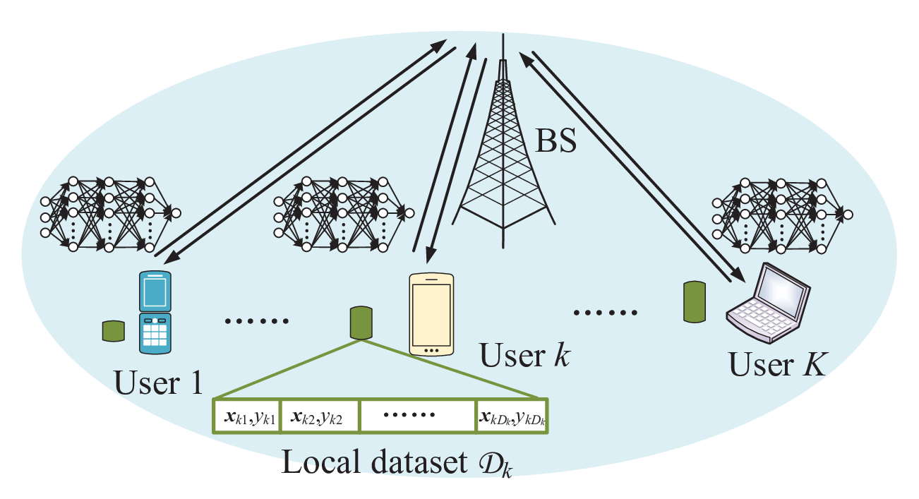
Consider a cellular network that consists of one BS serving a set of users, as shown in Fig. 1. Each user has a local dataset with data samples. For each dataset , is an input vector of user and is its corresponding output11 1 For simplicity, this paper only considers an FL algorithm with a single output. Our approach can be extended to the case with multiple outputs (Konečnỳ et al. 2016)..
2.1 FL Model
For FL, we define a vector to capture the parameters related to the global FL model that is trained by all datasets. Hereinafter, the FL model that is trained by all users’ data set is called global FL model, while the FL model that is trained by each user’s dataset is called local FL model. We introduce the loss function , that captures the FL performance over input vector and output . For different learning tasks, the loss function will be different. Since the dataset of user is , the total loss function of user will be:
| (1) |
In order to deploy FL, it is necessary to train the underlying model. Training is done in order to compute the global FL model for all users without sharing their local datasets due to privacy and communication issue. The FL training problem can be formulated as follows (Wang et al. 2018):
| (2) |
where is the total data samples of all users.
To solve problem (2), we adopt the FL algorithm in (Konečnỳ et al. 2016), which is summarized in Algorithm 1.
In Algorithm 1, at each iteration of the FL algorithm, each user downloads the global FL model parameters from the BS for local computing, while the BS periodically gathers the local FL model parameters from all users and sends the updated global FL model parameters back to all users. We define as the global FL parameter at a given iteration . Each user computes the local FL problem:
| (3) |
by using the gradient method with a given accuracy. In problem (2.1), is a constant value. The solution in problem (2.1) means the updated value of local FL parameter for user in each iteration, i.e., denotes user ’ local FL parameter at the -th iteration. Since it is hard to obtain the actual optimal solution of problem (2.1), we obtain a solution of (2.1) with some accuracy. The solution of problem (2.1) at the -th iteration with accuracy means that
| (4) |
where is the actual optimal solution of problem (2.1).
In Algorithm 1, the iterative method involves a number of global iterations (i.e., the value of in Algorithm 1) to achieve a global accuracy of global FL model. The solution of problem (2) with accuracy means that
| (5) |
where is the actual optimal solution of problem (2).
To analyze the convergence of Algorithm 1, we assume that is -Lipschitz continuous and -strongly convex, i.e.,
| (6) |
Under assumption (6), we provide the following lemma about convergence rate of Algorithm 1.
Lemma 1
If we run Algorithm 1 with for
| (7) |
iterations with , we have .
The proof of Lemma 1 can be found in (Yang et al. 2019). From Lemma 1, we can find that the number of global iterations increases with the local accuracy. This is because more iterations are needed if the local computation has a low accuracy.
2.2 Computation and Transmission Model
The FL procedure between the users and their serving BS consists of three steps in each iteration: Local computation at each user (using several local iterations), local FL parameter transmission for each user, and result aggregation and broadcast at the BS. During the local computation step, each user calculates its local FL parameters by using its local dataset and the received global FL parameters.
2.2.1 Local Computation
We solve the local learning problem (2.1) by using the gradient method. In particular, the gradient procedure in the -th iteration is given by:
| (8) |
where is the step size, is the value of at the -th local iteration with given vector , and is the gradient of function at point . We set the initial solution .
Next, we provide the number of local iterations needed to achieve a local accuracy in (2.1). We set .
Lemma 2
If we set step and run the gradient method for iterations at each user, we can solve local FL problem (2.1) with an accuracy .
The proof of Lemma 2 can be found in paper (Yang et al. 2019). Let be the computation capacity of user , which is measured by the number of CPU cycles per second. The computation time at user needed for data processing is:
| (9) |
where (cycles/bit) is the number of CPU cycles required for computing one sample data at user , is the number of local iterations for each user as given by Lemma 2, and .
2.2.2 Wireless Transmission
After local computation, all users upload their local FL parameters to the BS via frequency domain multiple access (FDMA). The achievable rate of user can be given by:
| (10) |
where is the bandwidth allocated to user , is the transmit power of user , is the channel gain between user and the BS, and is the power spectral density of the Gaussian noise. Due to the limited bandwidth, we have where is the total bandwidth.
In this step, user needs to upload the local FL parameters to the BS. Since the dimensions of the vector are fixed for all users, the data size that each user needs to upload is constant, and can be denoted by . To upload data of size within transmit time , we must have:
2.2.3 Information Broadcast
In this step, the BS aggregates the global prediction model parameters. The BS broadcasts the global prediction model parameters to all users in the downlink. Due to the high power of the BS and large downlink bandwidth, we ignore the downlink time. Note that the local data is not accessed by the BS, so as to protect the privacy of users, as is required by FL. The delay of each user includes the local computation time and transmit time. Based on (7) and (9), the delay of user will be:
| (11) |
We define as the delay for training the whole FL algorithm.
2.3 Problem Formulation
We now pose the delay minimization problem:
| (12) | ||||
| s.t. | (12a) | |||
| (12b) | ||||
| (12c) | ||||
| (12d) | ||||
| (12e) | ||||
| (12f) | ||||
where , , , and . and are, respectively, the maximum local computation capacity and maximum transmit power of user . (12a) indicates that the execution time of the local tasks and the transmit time for all users should not exceed the delay of the whole FL algorithm. The data transmission constraint is given by (12b), while the bandwidth constraint is given by (12c). (12d) represents the maximum local computation capacity and transmit power limits of all users. The accuracy constraint is given by (12e).
3 Optimal Resource Allocation
Although the delay minimization problem (12) is nonconvex due to constraints (12a)-(12b), the globally optimal solution is shown to be obtained by using the bisection method.
3.1 Optimal Resource Allocation
Let be the optimal solution of problem (12). We provide the following lemma about the feasibility conditions of problem (12).
Proof: Assume that is a feasible solution of problem (12) with . Then, solution is feasible with lower value of the objective function than solution , which contradicts the fact that is the optimal solution. For problem (12) with , we can always construct a feasible solution to problem (12) by checking all constraints.
According to Lemma 3, we can use the bisection method to obtain the optimal solution of problem (12). Denote
| (13) |
If , problem (12) is always feasible by setting , , , , and
| (14) |
Hence, the optimal of problem (12) must lie in the interval . At each step, the bisection method divides the interval in two by computing the midpoint . There are now only two possibilities: 1) if problem (12) with is feasible, we have and 2) if problem (12) with is infeasible, we have . The bisection method selects the subinterval that is guaranteed to be a bracket as the new interval to be used in the next step. As such an interval that contains the optimal is reduced in width by 50% at each step. The process continues until the interval is sufficiently small.
With a fixed , we still need to check whether there exists a feasible solution satisfying constraints (12a)-(12g). From constraints (12a) and (12c), we can see that it is always efficient to utilize the maximum computation capacity, i.e., . In addition, from (12b) and (12d), we can see that minimizing the delay can be done by having: . Substituting the maximum computation capacity and maximum transmission power into (12), delay minimization problem becomes:
| (15) | ||||
| s.t. | (15a) | |||
| (15b) | ||||
| (15c) | ||||
| (15d) | ||||
| (15e) | ||||
We provide the sufficient and necessary condition for the feasibility of set (15a)-(15e) using the following lemma.
Proof: To prove this, we first define a function with . Then, we have
| (19) |
According to (19), is a decreasing function. Since , we have for all . Hence, is an increasing function, i.e., the right hand side of (15b) is an increasing function of bandwidth . To ensure that the maximum bandwidth constraint (15c) can be satisfied, the left hand side of (15b) should be as small as possible, i.e., should be as long as possible. Based on (15a), the optimal time allocation should be:
| (20) |
Substituting (20) into (15b), we can construct the following problem:
| (21) | ||||
| s.t. | (21a) | |||
| (21b) | ||||
| (21c) | ||||
where is defined in (18). We can observe that set (15a)-(15e) is nonempty if an only if the optimal objective value of (21) is less than . Since the right hand side of (15b) is an increasing function, (15b) should hold with equality for the optimal solution of problem (21). Setting (15b) with equality, problem (21) reduces to (16).
Lemma 5
In (17), is a convex function.
Proof: We first prove that is a convex function. To show this, we define:
| (22) |
and
| (23) |
According to (18), we have: Then, the second-order derivative of can be given by:
| (24) |
According to (22) and (23), we have:
| (25) |
and
| (26) |
Combining (24)-(26), we can find that , i.e., is a convex function.
Then, we can show that is an increasing and convex function. According to the proof of Lemma 4, is the inverse function of the right hand side of (15b). If we further define function:
| (27) |
is the inverse function of , which gives .
According to (19), function is an increasing and concave function, i.e., and . Since is an increasing function, its inverse function is also an increasing function.
Based on the definition of concave function, for any , and , we have:
| (28) |
Applying the increasing function on both sides of (28) yields:
| (29) |
Denote and , i.e., we have and . Thus, (29) can be rewritten as:
| (30) |
which indicates that is a convex function. As a result, we have proven that is an increasing and convex function, which shows:
| (31) |
Lemma 5 implies that the optimization problem in (16) is a convex problem, which can be effectively solved. By finding the optimal solution of (16), the sufficient and necessary condition for the feasibility of set (15a)-(15e) can be simplified using the following theorem.
Theorem 1 directly follows from Lemmas 4 and 5. Due to the convexity of function , is an increasing function of . As a result, the unique solution of to can be effectively solved via the bisection method.
Based on Theorem 1, the algorithm for obtaining the minimal delay is summarized in Algorithm 2.
4 Simulation Results
For our simulations, we deploy users uniformly in a square area of size m m with the BS located at its center. The path loss model is ( is in km) and the standard deviation of shadow fading is dB (Yang et al. 2020). In addition, the noise power spectral density is dBm/Hz. We use the real open blog feedback dataset in (Buza 2014). This dataset with a total number of 60,021 data samples originates from blog posts and the dimensional of each data sample is 281. The prediction task associated with the data is the prediction of the number of comments in the upcoming 24 hours. Parameter is uniformly distributed in cycles/sample. The effective switched capacitance in local computation is . In Algorithm 1, we set , , and . Unless specified otherwise, we choose an equal maximum average transmit power dBm, an equal maximum computation capacity GHz, a transmit data size kbits, and a bandwidth MHz. Each user has data samples, which are randomly selected from the dataset with equal probability. All statistical results are averaged over 1000 independent runs.

In Fig. 2, we show the value of the loss function as the number of iterations varies for convex and nonconvex loss functions. For this feedback prediction problem, we consider two different loss functions: convex loss function , and nonconvex loss function . From this figure, we can see that, as the number of iterations increases, the value of the loss function first decreases rapidly and then decreases slowly for both convex and nonconvex loss functions. According to Fig. 2, the initial value of the loss function is and the value of the loss function decreases to for convex loss function after 500 iterations. For our prediction problem, the optimal model is the one that predicts the output without any error, i.e., the value of the loss function value should be . Thus, the actual accuracy of the proposed algorithm is after 500 iterations. Meanwhile, Fig. 2 clearly shows that the FL algorithm with a convex loss function can converge faster than that the one having a nonconvex loss function. According to Fig. 2, the loss function monotonically decreases as the number of iterations varies for even nonconvex loss function, which indicates that the proposed FL scheme can also be applied to the nonconvex loss function.

We compare the proposed FL scheme with the FL FDMA scheme with equal bandwidth (labelled as ‘EB-FDMA’), the FL FDMA scheme with fixed local accuracy (labelled as ‘FE-FDMA’), and the FL time division multiple access (TDMA) scheme in (Tran et al. 2019) (labelled as ‘TDMA’). Fig. 3 shows how the delay changes as the maximum average transmit power of each user varies. We can see that the delay of all schemes decreases with the maximum average transmit power of each user. This is because a large maximum average transmit power can decrease the transmission time between users and the BS. We can clearly see that the proposed FL scheme achieves the best performance among all schemes. This is because the proposed approach jointly optimizes bandwidth and local accuracy , while the bandwidth is fixed in EB-FDMA and is not optimized in FE-FDMA. Compared to TDMA, the proposed approach can reduce the delay by up to 27.3%.
5 Conclusions
In this paper, we have investigated the delay minimization problem of FL over wireless communication networks. The tradeoff between computation delay and transmission delay is determined by the learning accuracy. To solve this problem, we first proved that the total delay is a convex function of the learning accuracy. Then, we have obtained the optimal solution by using the bisection method. Simulation results show the various properties of the proposed solution.
References
- Ahn et al. (2019) Ahn, J.-H., Simeone, O., and Kang, J. Wireless federated distillation for distributed edge learning with heterogeneous data. arXiv preprint arXiv:1907.02745, 2019.
- Buza (2014) Buza, K. Feedback prediction for blogs. In Data analysis, machine learning and knowledge discovery, pp. 145–152. Springer, 2014.
- Chen et al. (2019a) Chen, M., Challita, U., Saad, W., Yin, C., and Debbah, M. Artificial neural networks-based machine learning for wireless networks: A tutorial. IEEE Commun. Surveys Tut., pp. 1–1, 2019a. ISSN 1553-877X. doi: 10.1109/COMST.2019.2926625.
- Chen et al. (2019b) Chen, M., Yang, Z., Saad, W., Yin, C., Poor, H. V., and Cui, S. Performance optimization of federated learning over wireless networks. In Proc. IEEE Global Commun. Conf., pp. 1–6, Waikoloa, HI, USA, Dec. 2019b.
- Chen et al. (2019) Chen, M., Yang, Z., Saad, W., Yin, C., Poor, H. V., and Cui, S. A joint learning and communications framework for federated learning over wireless networks. arXiv preprint arXiv:1909.07972, 2019.
- Chen et al. (2020) Chen, M., Semiari, O., Saad, W., Liu, X., and Yin, C. Federated echo state learning for minimizing breaks in presence in wireless virtual reality networks. IEEE Trans. Wireless Commun., to appear, 2020.
- Dong et al. (2019) Dong, P., Zhang, H., Li, G. Y., Gaspar, I. S., and NaderiAlizadeh, N. Deep CNN-based channel estimation for mmWave massive MIMO systems. IEEE J. Sel. Topics Signal Process., 13(5):989–1000, Sept. 2019.
- Gao et al. (2020) Gao, S., Dong, P., Pan, Z., and Li, G. Y. Reinforcement learning based cooperative coded caching under dynamic popularities in ultra-dense networks. IEEE Trans. Veh. Technol., 69(5):5442–5456, 2020.
- Gündüz et al. (2019) Gündüz, D., de Kerret, P., Sidiropoulos, N. D., Gesbert, D., Murthy, C. R., and van der Schaar, M. Machine learning in the air. IEEE J. Sel. Areas Commun., 37(10):2184–2199, Oct. 2019.
- Huang et al. (2020) Huang, C., Mo, R., and Yuen, C. Reconfigurable intelligent surface assisted multiuser MISO systems exploiting deep reinforcement learning. IEEE J. Sel. Areas Commun., pp. 1–1, 2020.
- Konečnỳ et al. (2016) Konečnỳ, J., McMahan, H. B., Ramage, D., and Richtárik, P. Federated optimization: Distributed machine learning for on-device intelligence. arXiv preprint arXiv:1610.02527, 2016.
- McMahan et al. (2016) McMahan, H. B., Moore, E., Ramage, D., Hampson, S., and Arcas, B. A. y. Communication-efficient learning of deep networks from decentralized data. arXiv preprint arXiv:1602.05629, 2016.
- Park et al. (2019) Park, J., Samarakoon, S., Bennis, M., and Debbah, M. Wireless network intelligence at the edge. Proceedings of the IEEE, 107(11):2204–2239, Nov. 2019.
- Saad et al. (to appear, 2020) Saad, W., Bennis, M., and Chen, M. A vision of 6G wireless systems: Applications, trends, technologies, and open research problems. IEEE Network, to appear, 2020.
- Samarakoon et al. (2018) Samarakoon, S., Bennis, M., Saad, W., and Debbah, M. Distributed federated learning for ultra-reliable low-latency vehicular communications. arXiv preprint arXiv:1807.08127, 2018.
- Tran et al. (2019) Tran, N. H., Bao, W., Zomaya, A., and Hong, C. S. Federated learning over wireless networks: Optimization model design and analysis. In Proc. IEEE Conf. Computer Commun., pp. 1387–1395, Paris, France, June 2019.
- Wang et al. (2018) Wang, S., Tuor, T., Salonidis, T., Leung, K. K., Makaya, C., He, T., and Chan, K. When edge meets learning: Adaptive control for resource-constrained distributed machine learning. In IEEE Conf. Computer Commun., pp. 63–71, Honolulu, HI, USA, Apr. 2018.
- Wang et al. (2019) Wang, S., Tuor, T., Salonidis, T., Leung, K. K., Makaya, C., He, T., and Chan, K. Adaptive federated learning in resource constrained edge computing systems. IEEE J. Sel. Areas Commun., 37(6):1205–1221, June 2019.
- Yang et al. (2020) Yang, H. H., Liu, Z., Quek, T. Q. S., and Poor, H. V. Scheduling policies for federated learning in wireless networks. IEEE Trans. Commun., to appear, 2020.
- Yang et al. (2018) Yang, K., Jiang, T., Shi, Y., and Ding, Z. Federated learning via over-the-air computation. arXiv preprint arXiv:1812.11750, 2018.
- Yang et al. (2019) Yang, Z., Chen, M., Saad, W., Hong, C. S., and Shikh-Bahaei, M. Energy efficient federated learning over wireless communication networks. arXiv preprint arXiv:1911.02417, 2019.
- Yang et al. (2020) Yang, Z., Chen, M., Saad, W., Xu, W., Shikh-Bahaei, M., Poor, H. V., and Cui, S. Energy-efficient wireless communications with distributed reconfigurable intelligent surfaces, 2020.
- Zeng et al. (2019) Zeng, Q., Du, Y., Leung, K. K., and Huang, K. Energy-efficient radio resource allocation for federated edge learning. arXiv preprint arXiv:1907.06040, 2019.
- Zhu et al. (2018a) Zhu, G., Liu, D., Du, Y., You, C., Zhang, J., and Huang, K. Towards an intelligent edge: Wireless communication meets machine learning. arXiv preprint arXiv:1809.00343, 2018a.
- Zhu et al. (2018b) Zhu, G., Wang, Y., and Huang, K. Low-latency broadband analog aggregation for federated edge learning. arXiv preprint arXiv:1812.11494, 2018b.