On some conditionally solvable quantum-mechanical problemsThanks: e–mail: fernande@quimica.unlp.edu.ar

In addition to the exactly solvable quantum-mechanical models, like the harmonic oscillator and the hydrogen atom, among others, where one obtains the whole spectrum for any values of the model parameters[1, 2], there is the class of quasi-solvable or conditionally-solvable systems where one obtains a subset of eigenvalues and eigenfunctions in exact analytical way only for some values of the model parameters or suitable constrains for them[3, 4, 5, 6, 7, 12, 8, 9, 10, 11, 13, 14, 15, 16, 17]. The most widely studied models are anharmonic oscillators[3, 4, 5, 6, 7, 8, 10, 11, 13, 14, 15, 16] and perturbed Coulomb systems[9, 13, 15, 16, 17].

The perturbed Coulomb system appears in the analysis of a variety of physical problems and enabled some researchers to predict the existence of allowed cyclotron frequencies, allowed field intensities, etc[18, 19, 20, 21, 22, 23, 24, 25, 26, 27, 28, 29, 30].

The purpose of this paper is the analysis of two conditionally solvable models that can be reduced to a three-term recurrence relation. In Sec. 2 we outline the main features of the three-term recurrence relation, in sections 3 and 4 we show diagrams for the distribution of the eigenvalues of a sextic anharmonic oscillator and a perturbed Coulomb model, respectively. We comment on the wrong interpretation of the eigenvalues obtained by several authors for the latter example. Finally, in Sec. 5 we summarize the main results and draw conclusions.

Consider a Schrödinger equation

with a Hamiltonian operator $H=H(\mathbf{a})$ that depends on a set of model parameters $\mathbf{a}=\left(a_{1},a_{2},\ldots a_{K}\right)$. Suppose that we can write the solution $\psi$ as a linear combination of a (not necessarily orthonormal) basis set $\left\{\varphi_{j},\,j=0,1,\ldots\right\}$

so that the coefficients $c_{j}$ obey a three-term recurrence relation

Some authors state that the expansion coefficients are normalization constants[15, 16].

If the equations

can be solved for $E$ and $\mathbf{a}$ for some $n$, then $c_{j}=0$ for all $j>n$. If the solutions to these equations are physically acceptable then we have obtained an exact solution to the Schrödinger equation (1). More precisely, we would have obtained $E=E^{(n)}(\mathbf{a}_{n})$, where the set of parameters $\mathbf{a}_{n}$ is a solution to some nonlinear equation $F_{n}\left(\mathbf{a}_{n}\right)=0$. Clearly, the model parameters $\mathbf{a}_{n}$ that satisfy this condition will not be independent. The truncation condition (4) is equivalent to

This truncation condition proposed by Verçin[18] for a particular problem appears to be simpler than the determinantal condition used by other authors[11, 14].

The coefficients $\hat{c}_{j}=(-1)^{j}c_{j}$ satisfy

that will be useful for the interpretation of some of the results below.

As a first example we consider the anharmonic oscillator

that supports bound states for all real values of the parameters $a$ and $b$. In earlier treatments of the sextic oscillator the authors considered a positive coefficient for the sextic term[3, 4, 5, 6, 7, 8, 10, 11, 13, 14, 15, 16]. However, such a coefficient can be easily set to unity by means of a suitable change of the independent variable $x$[31]. For this reason we choose the coefficient of $x^{6}$ equal to unity without loss of generality.

We have three cases:

Case I: $4a+b^{2}<0\Rightarrow$ single well

Case II: $4a+b^{2}>0,\,a>0\Rightarrow$ double well

Case III: $4a+b^{2}>0,\,a<0\Rightarrow$ triple well

A suitable non-orthogonal basis set for the treatment of this problem is

where $s=0$ or $s=1$ for even or odd states, respectively. A straightforward calculaton leads to

From $B_{n+1}=0$ we obtain a relationship for the model parameters

from which we obtain either $a(b)$ or $b(a)$. Notice that the truncation condition gives us the possibility of double and triple wells.

The truncation condition (5) leads to an exact eigenfunction

If we solve equation (10) for $a$ we obtain $a_{n,s}(b)$ and a Hamiltonian operator $H_{n,s}$ that depends on this particular relationship between $a$ and $b$. It is worth having in mind that $\psi_{s}^{(n)}(x)$ and $\psi_{s^{\prime}}^{(n^{\prime})}(x)$ are not eigenfunctions of the same hamiltonian but of $H_{n,s}$ and $H_{n^{\prime},s^{\prime}}$, respectively, which are two different operators. We are not being unnecessarily careful about this point because it has been misunderstood by other authors[18, 19, 20, 21, 22, 23, 24, 25, 26, 27, 28, 29, 30].

For example, for $n=0$ we obtain

Since $c_{s,j}^{(0)}=0$ for all $j>0$ the corresponding function has no nodes when $s=0$ and only one node at $x=0$ when $s=1$. The former is the ground state for the model determined by $a_{0,0}(b)$ and the latter is the first-excited state for $a_{0,1}(b)$.

For $n=1$ we have two solutions

The values of the coefficient $c_{1}$ in these two cases are

Since $c_{0,s,1}^{(1)}>0$ and $c_{1,s,1}^{(2)}<0$ we conclude that they are consistent with the first two even states of $H_{1,0}$ and the fist two odd states of $H_{1,1}$.

For $n=2$ we have three eigenvalues for just one value of $a$

The three roots $E_{0,s}^{(2)}<E_{1,s}^{(2)}<E_{2,s}^{(2)}$ are three eigenvalues of the anharmonic oscillator $H_{2,s}$, even states for $s=0$ and odd ones for $s=1$. In general we expect $n+1$ energy eigenvalues $E_{i,s}^{(n)}$, $i=0,1,\ldots,n$ for the model given by the curve $a_{n,s}(b)$. In Appendix A we prove that all the roots $E_{i,s}^{(n)}$ are real. Notice that we have chosen the subscripts so that the eigenfunction $\psi_{i,s}^{(n)}(x)$ has exactly $i+s$ nodes and we can consider both $i$ and $s$ to be quantum numbers. In other words, we can label the eigenfunctions and eigenvalues of the Hamiltonian operator (7) as $\psi_{i,s}(x)$ and $E_{i,s}(a,b)$, respectively. On the other hand, the integer $n$ cannot be considered a quantum number as it merely indicates a given relationship $F_{n,s}(a,b)=0$ between the parameters $a$ and $b$ from which we obtain either $a_{n,s}(b)$ or $b_{n,s}(a)$ and the Hamiltonian operator $H_{n,s}$. Although the truncation condition (5) leads to a Hamiltonian operator that depends on $s$, this integer is actually a quantum number associated to the parity of the eigenfunction. For example, the well known eigenvalues $E_{\nu}=\hbar\omega\left(\nu+\frac{1}{2}\right)$, $\nu=0,1,\ldots$ of the harmonic oscillator can be written as $E_{i,s}=\hbar\omega\left(2i+s+\frac{1}{2}\right)$, $i=0,1,\ldots$, $s=0,1$.

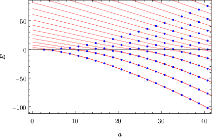
Figure 1 shows the eigenvalues $E_{\nu,s}(0,b)$ obtained from the truncation condition (blue circles) and those calculated by means of two variational methods[32, 33] (red lines). The potential-energy function $V(0,b,x)$ is a single well for $b<0$ and a double well for $b>0$. Since the depth of the wells increases with $b$ one expects negative eigenvalues for sufficiently large values of $b$. Straightforward calculation using the Riccati-Padé method (RPM)[34] shows that the first eigenvalue becomes negative at $b=2.491322600$ and the second one at $b=3.037089563$. There is a gap without blue points because the truncation condition requires that $b^{2}\geq 12$. Notice the coalescence of pairs of even and odd states as the wells become deeper. The members of such pairs approach each other when $b$ increases.

The symmetry of Figure 1 can be easily explained by an argument similar to that given by Child et al[14] for the central-field version of this model. To this end, notice that $A_{j}(-b,-E)=-A_{j}(b,E)$ and $B_{j}(a,-b)=B_{j}(a,b)$ leads to equation (6) with solutions $\hat{c}_{j}$. It is worth mentioning that the roots of the Hankel-Hadamard determinants in the Riccati-Padé method (RPM)[34] yield the eigenvalues for $b>0$ and $b<0$ simultaneously.

Figure 2 shows eigenvalues $E_{\nu,s}(a,0)$ obtained in the same way. The behaviour of these eigenvalues is similar to those in the previous case, except for the lack of symmetry. In this case the first eigenvalue becomes negative at $a=3$ and the second one at $a=5$.

Figure 3 shows eigenvalues $E_{\nu,s}(a,1)$. The first eigenvalue becomes negative at $a=1.901043863$ and the second one at $a=3.508348408$.

The behaviour of the eigenvalues $E_{\nu,s}(a,b)$ with respect to the model parameters $a$ and $b$ is given by the celebrated Hellmann-Feynman theorem[35] (and references therein)

The second example is given by the Hamiltonian operator

where $\gamma>0$ and $a$ and $b$ are real. Notice that this form of the Hamiltonian operator is suitable for the treatment of the central field model in any number of spatial dimensions. In fact, $\gamma$ may be a function of the number of spatial dimensions $D$ and the rotational quantum number $l$[13, 15, 16, 17] and may even take into account a term in the potential-energy function that behaves as $r^{-2}$ at origin[9].

A suitable basis set for this problem is

and we obtain the three-term recurrence relation (3) with

From $B_{n+1}=0$ we obtain an expression for the energy

and the truncation condition (5) leads to wavefunctions of the form

For simplicity, we label both the eigenvalues and eigenfunctions with the real number $\gamma$ although in general it will not be a true quantum number. We follow this practice because the form of $\gamma$ changes from one model to another and it will commonly depend on the angular quantum number[9, 13, 15, 16, 17].

For $n=0$ we have

and the corresponding wavefunction $\psi_{\gamma}^{(0)}$ does not have nodes.

For $n=1$ we have

The wave function for $a_{\gamma}^{(1,1)}$ will not have nodes in the interval $0<r<\infty$ because

is always positive. On the other hand, for the model $a_{\gamma}^{(1,2)}(b)$ we have one node in that interval because

is always negative.

For $n=2$ we have

In the general case we obtain $E_{\gamma}^{(n)}$ and $a_{n,\gamma}^{(i)}(b)$, $i=1,2,\ldots,n+1$, $a_{n,\gamma}^{(i+1)}(b)>a_{n,\gamma}^{(i)}(b)$. In Appendix A we prove that all the roots $a_{n,\gamma}^{(i)}(b)$ are real. In order to understand the relationship between these results and the actual eigenvalues $E_{\nu,\gamma}(a,b)$, $\nu=0,1,\ldots$ of the operator (17) we resort to the Hellmann-Feynman theorem that in this case states that

Since $E$ decreases with $a$ we conclude that the pair $\left[E_{\gamma}^{(n)},a_{n,\gamma}^{(i)}(b)\right]$ is a point on the curve $E_{i-1,\gamma}(a,b)$ for $a=a_{n,\gamma}^{(i)}(b)$.

It is clear that $\left[E_{\gamma}^{(n)},\psi_{\gamma}^{(n)}\right]$ is a pair of eigenvalue-eigenfunction of the operator $H_{n,\gamma}$, and that $\left[E_{\gamma^{\prime}}^{(n^{\prime})},\psi_{\gamma^{\prime}}^{(n^{\prime})}\right]$ corresponds to $H_{n^{\prime},\gamma^{\prime}}$. This apparently obvious fact has been misunderstood in many papers and the belief that $E_{\gamma}^{(n)}$ gives us the spectrum of a single quantum-mechanical system has led to the wrong conclusion that there exist allowed cyclotron frequencies, allowed field intensities and the like[18, 19, 20, 21, 22, 23, 24, 25, 26, 27, 28, 29, 30]. Such wrong conjectures arise from the belief that there are no square-integrable solutions outside those given by the truncation condition (5). This misinterpretation of the meaning of the exact solutions to conditionally solvable models has led to the fictitious dependence of frequencies and field intensities on the quantum numbers through, for instance, the parameter $a_{n,\gamma}$.

Figure 4 shows some eigenvalues for $\gamma=1$, $b=1$ in a range of values of $a$ calculated by the truncation condition (5) and a variational method with the nonorthogonal basis set of functions (18).

Although there have been several excellent papers published on the subject of conditionally solvable models[3, 4, 5, 6, 7, 12, 8, 9, 10, 11, 13, 17] we have decided to write the present one because the meaning of the exact solutions obtained for such particular models have not been understood[18, 19, 20, 21, 22, 23, 24, 25, 26, 27, 28, 29, 30]. These authors believe that the exact solutions to conditionally solvable models are the only bound states supported by them and, as a consequence, draw wrong conjectures such as the existence of allowed cyclotron frequencies, allowed field intensities and the like. These wrong conclusions stem from the fact that the exact solutions (with polynomial factors) are possible for some particular values of the model parameters. The dependence of the model parameters on the truncation number $n$ (the degree of the polynomial factor) has been interpreted as the dependence of the parameters on the quantum numbers and thereby the conclusion that bound states exist only for particular value of certain experimental quantities. This wrong interpretation of the truncation method has led them to believe that they obtained the whole spectrum of a given model when they obtained just one (in our second example) or a few (in our first example) energy for a given model. We hope to have made this point clear in the present paper.

The paper of Child et al[14] reveals a most clear picture of the distribution of the eigenvalues of the central-field sextic anharmonic oscillator, as well as a hidden symmetry. In this paper we add somewhat different diagrams of the distribution of the eigenvalues of conditionally solvable models that we believe to provide additional valuable information.

The research of P.A. was supported by Sistema Nacional de Investigadores (México).

References

- [1] L. D. Landau and E. M. Lifshitz, Quantum Mechanics. Non-relativistic Theory, (Pergamon, New York, 1958).
- [2] C. Cohen-Tannoudji, B. Diu, and F. Laloë, Quantum Mechanics, (John Wiley & Sons, New York, 1977).
- [3] G. P Flessas, Phys. Lett. A 72 (1979) 289-290.
- [4] G. P Flessas and K. P. Das, Phys. Lett. A 78 (1980) 19-21.
- [5] E. Magyari, Phys. Lett. A 81 (1981) 116-118.
- [6] G. P Flessas, J. Phys. A 14 (1981) L209-L211.
- [7] G. P Flessas, Phys. Lett. A 81 (1981) 17-18.
- [8] G. P Flessas and A. Watt, J. Phys. A 14 (1981) L315-L318.
- [9] A. DeSousa Dutra, Phys. Lett. A 131 (1988) 319-321.
- [10] R. S. Kaushal, Phys. Lett. A 142 (1989) 57-58.
- [11] S. K. Bose and N. Varma, Phys. Lett. A 147 (1990) 85-86.
- [12] P. Roy and Y. P. Varshni, Mod. Phys. Lett. A 6 (1991) 1257-1260.
- [13] R. N. Chaudhuri and M. Mondal, Phys. Rev. A 52 (1995) 1850-1856.
- [14] M. S. Child, S-H. Dong, and X-G. Wang, J. Phys. A 33 (2000) 5653-5661.
- [15] S-H. Dong, Phys. Scr. 65 (2002) 289-295.
- [16] S. M. Ikhdair and R. Sever, Int. J. Mod. Phys. C 18 (2007) 1571-1581.
- [17] S. Bera, B. Chakrabarti, and T. K. Das, Phys. Lett. A 381 (2017) 1356-1361.
- [18] A. Verçin, Phys. Lett. B 260 (1991) 120-124.
- [19] J. Myrheim, E. Halvorsen, and A. Verçin, Phys. Lett. B 278 (1992) 171-174.
- [20] C. Furtado, B. G. C da Cunha, F. Moraes, E. R. Bezerra de Mello, and V. B. Bezzerra, Phys. Lett. A 195 (1994) 90-94.
- [21] K. Bakke and F. Moraes, Phys. Lett. A 376 (2012) 2838-2841.
- [22] K. Bakke and H. Belich, Eur. Phys. J. Plus 127 (2012) 102.
- [23] K. Bakke, Ann. Phys. 341 (2014) 86-93.
- [24] K. Bakke, Int. J. Mod. Phys. A 29 (2014) 1450117.
- [25] K. Bakke and H. Belich, Eur. Phys. J. Plus 129 (2014) 147.
- [26] I. C. Fonseca and K. Bakke, J. Math. Phys. 56 (2015) 062107.
- [27] K. Bakke and C. Furtado, Ann. Phys. 355 (2015) 48-54.
- [28] E. R. Figueiredo Medeiros and E. R. Bezerra de Mello, Eur. Phys. J. C 72 (2012) 2051.
- [29] K. Bakke and H. Belich, Ann. Phys. (Berlin) 526 (2013) 187-194.
- [30] H. Hassanabadi, M. de Montigny, and M. Hosseinpour, Ann. Phys. 412 (2020) 168040.
- [31] F. M. Fernández, Dimensionless equations in non-relativistic quantum mechanics, arXiv:2005.05377 [quant-ph]
- [32] A. Okopinska, Phys. Rev.D 36 (1987) 1273-1275.
- [33] P. Amore, J. Phys. A 39 (2006) L349-L355.
- [34] F. M. Fernández, Q. Ma, and R. H. Tipping, Phys. Rev. A 39 (1989) 1605-1609.
- [35] F. L. Pilar, Elementary Quantum Chemistry, (McGraw-Hill, New York, 1968).