Twisting Neutral Particles with Electric Fields

First we will consider the longitudinal spin-orbit effect. We will assume that the extent of the electric field is semi-infinite and that it is parallel to the z-axis. Hence the Schroedinger equation can be written as

with $C=\frac{\gamma E_{z}}{c^{2}}$. The incident wave will be described by $\psi^{I}_{\pm}=f(r,\phi)e^{-ikz}$. Note that for a non-zero coupling this effect requires the incident wavefunction to have a transverse momentum component. By applying a Fourier transform over the x and y coordinates the PDE (Eq. 3) is simplified to a coupled second order ODE.

Here we have also transformed the equation to cylindrical coordinates with $k_{r}^{2}=k_{x}^{2}+k_{y}^{2}$ and $k_{x}\pm ik_{y}=k_{r}e^{\pm i\phi}$. It is noteworthy that in the spectral domain the potential, $C(k_{x}\sigma_{y}+k_{y}\sigma_{x})$, closely resembles that of the magnetic quadrupole in real space. This gives an intuitive reason as to why a static electric field mimics the action of a quadrupole in reciprocal space. Hence an electric field is more effective for large divergences (i.e. large $k_{r}$). We diagonalize equation 4, by applying a transformation of the form $\hat{\psi}=T\hat{\psi}^{\prime}$ and multiplying the Hamiltonian by $T^{-1}$ from the left.

For this particular diagonalization $T$ is given by $\begin{pmatrix}&ie^{-i\phi}\ \ &-ie^{-i\phi}\\ &1\ \ &1\end{pmatrix}$. The general solution to Eq. 5 is simply a superposition of a forward and backward propagating plane wave for each spin state

with $k_{\pm}=\sqrt{\epsilon-k_{r}^{2}\pm Ck_{r}}$. Amplitudes of the backward propagating solutions, $\hat{t}_{1}$ and $\hat{t}_{3}$, are zero. The general solution for $\hat{\psi}$ is simply found by applying the transformation $T\hat{\psi}^{\prime}$.

To determine the values of $\hat{t}_{2}$, $\hat{t}_{4}$ and the reflection coefficients $\hat{r}_{\pm}$ we apply the boundary conditions

Here the subscript $z$ under $\psi$ denotes the partial derivative to the $z$ coordinate. $\hat{f}_{\pm}(k_{r},\phi)$ denotes the 2D Fourier transform of the incident wavefunction. This boundary value problem can be formulated as the following matrix vector problem

By inverting the above 4x4 matrix we find the transmission and reflection coefficients

which leads us to the solution for the transmitted waves

Looking at this expression we can see that the total angular momentum $J=S+L$ of the wave is conserved in a static electric field, since a spin flip is compensated by a change in OAM.

$\hat{f}_{\pm}(k_{r},\phi)$ can be expanded such that $\hat{f}_{\pm}(k_{r},\phi)=\sum_{\ell}\hat{f}^{\ell}_{\pm}(k_{r})e^{i\ell\phi}$, where $\hat{f}_{\pm}^{l}(k_{r})$ is given by the azimuthal Fourier Transform

The solution in real space can be obtained by applying the Bessel/Hankel transform to Eq. 11.

It is instructive to look at the solution of Eq. 13 for an incident wavefield, $\psi^{I}_{\pm}$, described by a Bessel beam carrying no OAM, $\psi^{I}_{\pm}=b_{\pm}J(k_{\rho}r)e^{-ik_{z}z}$, with $b_{\pm}$ the amplitude of the up and down spin state respectively and $k_{\rho}$ the transverse momentum component of the incident wave. Hence $\hat{f}_{\pm}^{\ell\neq 0}=0$ and $\hat{f}_{\pm}^{0}(k_{r})=b_{\pm}\frac{\delta(k_{r}-k_{\rho})}{k_{r}}$ with $\epsilon=k_{z}^{2}+k_{\rho}^{2}$. In this case the solution is trivial

where $\psi_{\pm}^{0}$ and $\psi_{\pm}^{1}$ are the components with and without OAM respectively, such that $\psi_{\pm}=\psi_{\pm}^{0}+e^{\mp i\theta}\psi_{\pm}^{1}$. For a collimated beam geometry we may use $k_{\rho}=k_{z}\tan(\alpha)\approx k_{z}\alpha$, where $\alpha$ is the beam divergence. Furthermore if $Ck_{\rho}$ is sufficiently small we may linearize the square root terms in equation 14 and obtain a much simpler expression for the wavefunction.

A longitudinal beam twister device may be constructed using a parallel plate capacitor, with the surfaces of the plates normal to the beam. The voltage required to fully twist the beam from the $\ell=0$ state into the $\ell=\pm 1$ state is given by

These equations are valid for single Bessel beams. However Bessel functions are not normalizable Bliokh2017 and therefore have infinite coherence, making them unphysical. In a realistic setup we always have a normalizable superposition of Bessel beams, which have finite coherence. This superposition interferes and results in damping of spin orbit production, due to dephasing. This interference can be described by solving Eq. 13 for an arbitrary divergence profile. Though we can also determine the probability of the particle being in the mth OAM state as a function of $z$ without the inverse transform, Eq. 13, by simply calculating the projection of Eq. 11 on $e^{im\phi}$ and integrating the absolute value squared of this expression over $k_{r}$:

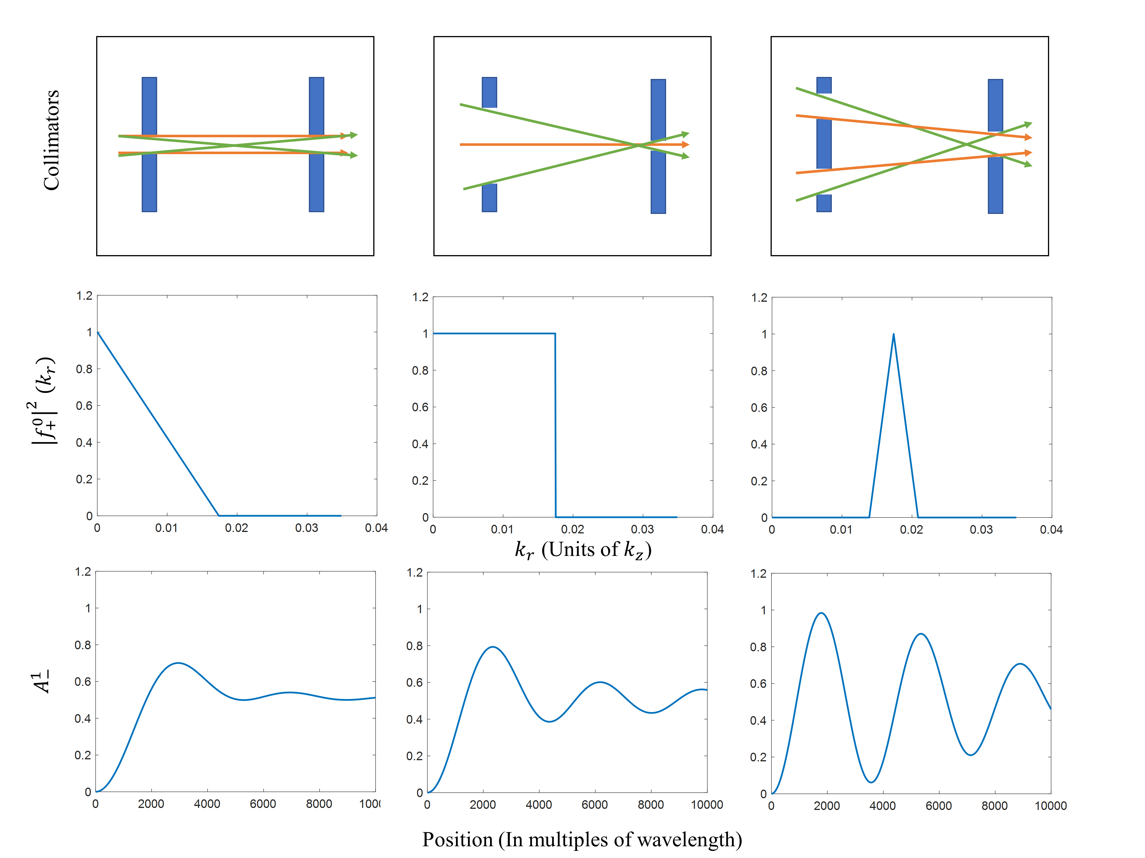
with $\hat{\psi}^{m}=<e^{im\phi}|\hat{\psi}>$, the azimuthal Fourier transform (eq. 12) of $\hat{\psi}$. Here we have also used Parsevals theorem to demonstrate that the value of $A^{m}$ is the same in real and reciprocal space. Solutions of equation 17 for the most common divergence profiles, $|f|^{2}(k_{r},\phi)$ are shown in figure 1. Here we see dephasing effects which causes the contrast of $A^{1}_{-}$ to wash out as the wave penetrates deeper into the electric field. As the transverse wavelength spread is decreased the dephasing effects are also reduced. This is analogous to dephasing seen in magnetic spin echo instruments, due to the longitudinal wavelength spread Mezei1980.

Equation 16 demonstrates that for particles with a divergence of $1^{\degree}$ propagating through a capacitor we require a voltage drop of $88.4GV$ to put a neutron into an OAM state with $\ell=\pm 1$. Obviously this is not feasible. For colder particles it is possible to use zone plates which consist of concentric rings of periodically spaced absorber material to increase the transverse momentum, $k_{r}$, thereby decreasing the required voltage drop. Such Fresnel lenses have been produced for the purpose of imaging with very cold neutrons Kearney1980.

Next we consider waves interacting with an electric field interface at grazing incidence angles. This results in a more pronounced coupling, due to a larger $k_{r}$ and a smaller value for $k_{z}$. The OAM carried by the transmitted and reflected waves in this case is quasi-transverse to the wavevector $\vec{k}$. Since the quantization axis of the OAM is normal to interface, the incident wave must be described by an infinite superposition of OAM modes. Nonetheless the mean OAM of the transmitted and reflected waves can be raised or lowered by one unit of $\hbar$ with respect to the incident OAM. The reflection probability $|r_{\pm}|^{2}$ as a function of incident angle is shown in Fig. 2, for an electric field of $10^{10}V/m$ (found in electric double layers Toney1995; Ferechmin2002), a neutron wavelength of $2$ Å and an initial spin aligned along the $-z$ direction. We can deduce that the optimal angle of reflection is around $0.001^{\degree}$. Hence this method of OAM generation is likely not feasible due to flux limitations.

The flux limitations can be overcome by considering transmission through a transversely polarized electric field which leads to the generation of transverse spin-orbit states. To demonstrate this we consider the time dependent Schroedinger equation for a neutral spin 1/2 particle in an electric field

Again we will assume that the electric field is polarized along the z-direction. However this time we will consider a field which extends infinitely in space. To reduce the problem to an ordinary differential equation we apply an unbounded Fourier transform to the spatial coordinates. In cylindrical coordinates this leads to

$\epsilon$ now denotes the kinetic energy parameter $k_{r}^{2}+k_{z}^{2}$. Once again we diagonalize this set of equations using the transform $\hat{\psi}=T\hat{\psi}^{\prime}$

Applying the initial conditions $\hat{\psi}_{\pm}(t=0)=\hat{a}_{\pm}(k_{r},\phi,k_{z})$ we can determine the homogeneous solution of equation 19.

which appears almost equivalent to equation 15. If the wave propagates along the y-direction the value of $k_{r}$, which may be approximated by $k_{y}$ is a factor $10^{2}-10^{3}$ larger than in the longitudinal case (equation 15). Hence the required electric field integral to raise or lower the mean OAM is reduced to a more practical level. The incident wave in this case must be described by an infinite superposition of transverse OAM modes. Upon being transmitted through an ideal beam twister device the mean $\ell$ value of this superposition will be raised or lowered by one. In this paper we assume that $\hat{a}_{\pm}$ can be approximated by a Gaussian model. The standard deviation in $k_{x}$ direction can be expressed in terms of a symmetry factor $R$ and the standard deviation in $k_{y}$ direction $\sigma_{y}$: $\sigma_{x}=R\sigma_{y}$. Such that $\hat{a}_{\pm}=e^{-\frac{(k_{y}-k_{y}^{\prime}).^{2}}{\sigma_{y}^{2}}}e^{-\frac{k_{x}^{2}}{R^{2}\sigma_{y}^{2}}}$, with $k_{y}^{\prime}$, the mean momentum in the y-direction. This Gaussian can be expanded in its various OAM components by means of the azimuthal Fourier transform.

Upon passing through an appropriate electric field the index $\ell$ is raised or lowered by 1. Using this and equation 17 the amplitude of the $\ell=1$ OAM mode, $A^{1}$, can be calculated. We may also define an OAM bandwidth in terms of the standard deviation

with $<L_{z}>=\sum_{\ell}\ell A^{\ell}$ and $<L_{z}^{2}>=\sum_{\ell}\ell^{2}A^{\ell}$. Both the OAM amplitude $A^{1}$ and the OAM bandwidth, $\sigma_{\ell}$, are shown as a function of the reciprocal longitudinal coherence length $\sigma_{y}$ and the symmetry factor $R$ in Fig. 3. One can see that a small coherence length (large $\sigma_{y}$) leads to a larger amplitude, $A^{1}$ and a tighter bandwidth, $\sigma_{\ell}$. Analogously a large symmetry factor $R$ corresponds (i.e. a large beam divergence) to a larger amplitude, $A_{1}$ and a small bandwidth, $\sigma_{\ell}$.

In Fig. 4 we show one such Gaussian wavepacket carrying transverse OAM in real space. The wavepacket with OAM appears to be displaced along the transverse axis, while along the longitudinal axis the wavepacket is shifted by $\pi/2$.