Automatic Ischemic Stroke Lesion Segmentation from Computed Tomography Perfusion Images by Image Synthesis and Attention-Based Deep Neural Networks Journal: Elsevier
Abstract
Ischemic stroke lesion segmentation from Computed Tomography Perfusion (CTP) images is important for accurate diagnosis of stroke in acute care units. However, it is challenged by low image contrast and resolution of the perfusion parameter maps, in addition to the complex appearance of the lesion. To deal with this problem, we propose a novel framework based on synthesized pseudo Diffusion-Weighted Imaging (DWI) from perfusion parameter maps to obtain better image quality for more accurate segmentation. Our framework consists of three components based on Convolutional Neural Networks (CNNs) and is trained end-to-end. First, a feature extractor is used to obtain both a low-level and high-level compact representation of the raw spatiotemporal Computed Tomography Angiography (CTA) images. Second, a pseudo DWI generator takes as input the concatenation of CTP perfusion parameter maps and our extracted features to obtain the synthesized pseudo DWI. To achieve better synthesis quality, we propose a hybrid loss function that pays more attention to lesion regions and encourages high-level contextual consistency. Finally, we segment the lesion region from the synthesized pseudo DWI, where the segmentation network is based on switchable normalization and channel calibration for better performance. Experimental results showed that our framework achieved the top performance on ISLES 2018 challenge and: 1) our method using synthesized pseudo DWI outperformed methods segmenting the lesion from perfusion parameter maps directly; 2) the feature extractor exploiting additional spatiotemporal CTA images led to better synthesized pseudo DWI quality and higher segmentation accuracy; and 3) the proposed loss functions and network structure improved the pseudo DWI synthesis and lesion segmentation performance. The proposed framework has a potential for improving diagnosis and treatment of the ischemic stroke where access to real DWI scanning is limited.
Keywords:
Ischemic stroke lesion , computed tomography perfusion , image synthesis , segmentation , deep learning1 Introduction
Stroke is the most common cerebrovascular disease and one of the primary causes of mortality and long-term disability worldwide (Kissela et al. 2012). Ischemic stroke is the most common type of stroke and accounts for 75-85% of all stroke cases, which is an obstruction of the cerebral blood supply and leads to tissue hypoxia (under-perfusion) and tissue death within few hours. The stages of stroke can be classified into acute (0 to 24h), sub-acute (24h to 2w) and chronic (2w) (González et al. 2011). Early diagnosis and treatment in the acute stage is critical for recovery of the stroke patient, and medical imaging is important for detection and quantitative assessment of stroke lesions, as well as eligible patient selection for thrombolysis or thrombectomy (Zaharchuk et al. 2012).
Among different medical imaging methods, Magnetic Resonance Imaging (MRI) sequences such as Fluid-Attenuated Inversion Recovery (FLAIR), T1 weighted, T2 weighted, and Diffusion-Weighted Imaging (DWI) are preferred imaging modalities for ischemic stroke lesions due to their good soft tissue contrasts. Especially, DWI is considered as the most sensitive method for detection of early acute stroke (Mezzapesa et al. 2006). However, MR imaging including DWI is relatively slow and often not accessible for acute stroke patients. Alternatively, Computed Tomography Perfusion (CTP) imaging offers insights into cerebral hemodynamics and enables differentiation of salvageable penumbra from irrevocably damaged infarct core (Donahue and Wintermark 2015). CTP has advantages in speed and cost, leading to higher availability in acute care units (Gillebert et al. 2014). In CTP imaging, a sequence of Computed Tomography Angiography (CTA) images (i.e., spatiotemporal 4D images) are acquired during the perfusion process, which results in perfusion parameter maps such as Cerebral Blood Flow (CBF), Cerebral Blood Volume (CBV), Mean Transit Time (MTT), Time to Peak (TTP, or Tmax) to help to identify ischemic stroke lesions. Examples of perfusion parameter maps of two ischemic stroke patients are shown in Fig 1.
Segmentation of stroke lesions from medical images can provide quantitative measurements of the lesion region, which is important for quantitative treatment decision procedures. Manual segmentation of the lesion is time-consuming with low inter-rater agreement, and automatic stroke lesion segmentation is more efficient and has a potential to provide more reliable and reproducible segmentation results (Maier et al. 2017).

Considering the limited speed and availability of MRI for acute stroke patients, we aim to segment ischemic stroke lesions automatically from CTP perfusion parameter maps, which has a potential for improving diagnosis and treatment of ischemic stroke in a timely fashion. However, this task is very difficult and the segmentation accuracy is confronted with a lot of challenges. First, the appearance of stroke lesions varies considerably at different time, even within the same clinical stage of stroke (González et al. 2011). Second, the lesions have a large variation of location, shape, size and appearance in the brain, as shown in Fig. 1. Some lesions may be aligned with the vascular supply territories while others may not. The size of some small lesions can be only few millimeters, and some large lesions may cover a complete hemisphere (Maier et al. 2017). The intensity is not homogeneous in the lesion region, and some other stroke-similar pathologies may lead to false positives in the segmentation result. Thirdly, compared with DWI, the perfusion parameter maps (CBF, CBV, MTT, and Tmax) are noisy with a lower spatial resolution, making it difficult to accurately identify the boundary of stroke lesions, as demonstrated in Fig. 1. In addition, the raw spatiotemporal 4D CTA images contain useful information of the ischemic stroke lesion but have a large data size. Using the perfusion parameter maps alone without considering the raw spatiotemporal CTA images may limit the segmentation accuracy, while directly taking raw spatiotemporal CTA images for lesion segmentation increases the computational cost. Therefore, extracting compact and useful features from the raw spatiotemporal CTA images is desirable for efficient and accurate ischemic stroke lesion segmentation.
Although automatic segmentation of ischemic stroke lesion has been widely studied, most of existing methods were proposed to deal with multi-modal MR images (Maier et al. 2017; Winzeck et al. 2018). Only few works have been reported on ischemic stroke lesion segmentation from CTP images (Gillebert et al. 2014; Yahiaoui and Bessaid 2016; Abulnaga and Rubin 2018). Some old-fashion methods such as template-based methods (Gillebert et al. 2014) and fuzzy C-Means (Yahiaoui and Bessaid 2016) are challenged by the complex appearance of stroke lesions. Recently, deep learning methods have achieved state-of-the-art performance for many medical image segmentation tasks (Shen et al. 2017), and have been applied to ischemic stroke lesion segmentation from CTP images (Pinheiro et al. 2018; Abulnaga and Rubin 2018; Vikas Kumar Anand et al. 2018). However, due to the above mentioned challenges, it remains difficult to segment the lesions directly from the perfusion parameter maps.
Inspired by the fact that ischemic stroke lesions in DWI are easier to identify and segment than those in perfusion parameter maps, it is desirable to synthesize pseudo DWI images from perfusion parameter maps to help the segmentation task. Though a lot of methods have been proposed for general medical image synthesis (Frangi et al. 2018), synthesizing images with lesions is still not well addressed (Roy et al. 2010), which is challenged by the complex variation of pathological lesions among patients. Especially, synthesizing pseudo DWI images from CTP images of ischemic stroke lesions has rarely been investigated.
This work is a substantial extension of our preliminary conference publication (Song and Huang 2018) that won the MICCAI 2018 ischemic stroke lesion segmentation (ISLES) challenge11 1 http://www.isles-challenge.org. In this paper, we provide detailed description and in-depth discussion of our segmentation framework and validate it with extensive experiments. The contribution of our work is summarized as follows.
First, we propose a novel elaborated framework for automatic ischemic stroke lesion segmentation from CTP images based on synthesized pseudo DWI. Compared with using only CTP perfusion parameter maps, our framework additionally exploits raw spatiotemporal CTA images for higher pseudo DWI synthesis quality and lesion segmentation accuracy. Second, to make use of the raw spatiotemporal CTA images more efficiently, we propose a feature extractor that obtains more compact and high-level representation of the CTA images automatically, which helps to reduce the required memory and computational time and improve the performance of our segmentation method. Thirdly, we propose a novel method to synthesis pseudo DWI images with ischemic stroke lesions. We employ a high-level similarity loss function to encourage the pseudo DWI to be close to the ground truth in terms of both local details and global context, and propose an attention-guided synthesis strategy so that the generator will focus more on the lesion part, which benefits the final segmentation. Last but not least, to segment lesions from our synthesized pseudo DWI, we propose a Convolutional Neural Network (CNN) with channel calibration and Switchable Normalization (SN) (Luo et al. 2018) that is suitable for small training batch size, and combine it with a novel attention-based and hardness-aware loss function that helps to obtain more accurate segmentation of ischemic stroke lesions. Experimental results show that our method achieved state-of-the-art performance on ISLES 2018 challenge and it outperformed direct segmentation from CTP perfusion parameter maps and contemporary image synthesis-based methods for ischemic stroke lesion segmentation from CTP images (Liu 2018).
2 Related Works
2.1 Ischemic Stroke Lesion Segmentation
Segmentation of ischemic stroke lesion from medical images has attracted increasing attentions in recent years (Rekik et al. 2012; Maier et al. 2017), and most of them focus on segmentation from MR images. For example, the ISLES 2015-2017 challenges aimed at ischemic stroke lesion segmentation from multi-modal MR images including T1, T1-contrast, FLAIR and DWI sequences (Maier et al. 2017; Winzeck et al. 2018). Some early works have used a range of methods for this segmentation task, such as Markov random field model (Kabir et al. 2007), level set (Feng et al. 2015), random forest (Mitra et al. 2014) and support vector machine (Maier et al. 2014). However, their accuracy is challenged by the complicated segmentation problem (Maier et al. 2015). Recently, deep learning has been increasingly used for ischemic stroke lesion segmentation with better performance. For example, Kamnitsas et al. 2017 proposed a dual pathway 3D CNN combined with fully connected Conditional Random Field (CRF) for brain lesion segmentation. Cui et al. 2019 proposed an adapted mean teacher model to learn from a combination of annotated and unannotated MR images for the segmentation task. Dolz et al. 2018 combined DWI and CTP to segment ischemic stroke lesions and used a densely connected UNet with Inception modules (Szegedy et al. 2016) to handle the variation of lesion size. Despite their good performance, these methods rely on MRI and cannot be directly applied to stroke lesion segmentation from CTP images.
There have been few works on the challenging task of segmentation of ischemic stroke lesion from CTA or CTP perfusion parameter maps (Rekik et al. 2012). Some early works used histogram-based classifiers (Rekik et al. 2012) or template-based voxel-wise comparison (Gillebert et al. 2014) to deal with this problem. Yahiaoui and Bessaid 2016 used a multi-scale contrast enhancement algorithm and fuzzy C-Means for this task. Recently, Abulnaga and Rubin 2018 used CNNs with pyramid pooling to combine global and local contextual information for this task, where a focal loss was employed to enable the CNNs to focus more on hard samples. However, due to the lower signal-to-noise ratio of CTP perfusion parameter maps compared with DWI, it remains challenging to automatically segment the ischemic stroke lesion from CTP images.
2.2 Cross-Modality Medical Image Synthesis
A range of works have investigated the problem of synthesizing medical images from another modality (Frangi et al. 2018). For example, Burgos et al. 2014 synthesized CT images from MRI through a multi-atlas information propagation scheme. Bahrami et al. 2016 used dictionary learning to synthesis 7T-like images from 3T MRI. Jog et al. 2017 used regression random forest to synthesize T2 and FLAIR images from T1 images. Deep learning methods have also been increasingly used for medical image synthesis (Ker et al. 2017), such as deep neural network-based synthesis methods (Nguyen et al. 2015) and deep adversarial learning-based approaches (Nie et al. 2018). However, most of existing works deal with general cross-modality image synthesis and have not well investigated the more challenging problem of synthesizing medical images with pathological lesions. Roy et al. 2010 used an atlas-based method to synthesize FLAIR images with white matter lesions. Chartsias et al. 2017 proposed a CNN for synthesizing multi-modal MR images of brain lesions. The effectiveness of these methods for pseudo DWI synthesis from CTP perfusion parameter maps of stroke lesions has rarely been demonstrated.
3 Method
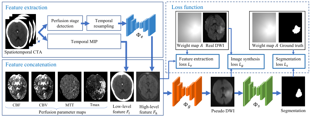
The proposed framework for ischemic stroke lesion segmentation from CTP images is depicted in Fig. 2. Due to the large inter-slice spacing (9.48 mm in average) of the experimental images, the proposed method operates on 2D slices. It consists of a feature extractor, a pseudo DWI generator and a final lesion segmenter. First, to efficiently deal with the large raw spatiotemporal CTA images and reduce the computational requirements, we design a high-level feature extractor that uses a CNN to obtain a compact representation of the raw spatiotemporal CTA images. Additionally, we make use of a temporal Maximal Intensity Projection (MIP) of the CTA images as a low-level feature. Then, these features are concatenated with the perfusion parameter maps to serve as the input of the pseudo DWI generator, which obtains a pseudo DWI image with better contrast between the lesion and the background. To improve the synthesis quality near lesion regions, we use a high-level similarity-based loss function and enable the generator to pay more attention to the lesion. Finally, a segmenter takes the pseudo DWI image as input and produces a segmentation of the ischemic stroke lesion, where a CNN using channel calibration and switchable normalization trained with an attention-based and hardness-aware loss function is proposed to improve the performance. The three components are trained end-to-end. Details of these components will be described in the following.
3.1 Feature Extraction from Raw Spatiotemporal CTA Images
In CTP imaging, the raw spatiotemporal CTA images have been transformed into a simplified feature representation in terms of perfusion parameter maps including CBF, CBV, MTT and Tmax. Though these parameter maps are useful for detection of the stroke lesion, they are not a complete representation of the perfusion information in the raw spatiotemporal CTA images. Therefore, we do not ignore the raw spatiotemporal CTA images and try to mine some additional features that are useful in the segmentation task.
Let represent a raw spatiotemporal CTA image obtained during the perfusion, where and is the total number of time points. Considering that the raw spatiotemporal CTA image has a large data size due to a large value of , we use a feature extractor to obtain an additional low-level feature and a compact and high-level representation of the raw spatiotemporal CTA image to make an efficient use of it. The feature extraction method is shown in Fig. 2. We extract both a manually designed low-level feature and a high-level feature that is automatically learned by a CNN.
First, the maximal intensity value of a voxel during perfusion may contain information related to the ischemic stroke lesion (Murayama et al. 2018). Therefore, in addition to the standard perfusion parameter maps, we apply a Maximal Intensity Projection (MIP) along the temporal axis to to obtain a low-level feature map :
| (1) |

Second, we use a CNN to extract high-level features of the raw spatiotemporal CTA image due to CNNs’ good performance in automatic feature extraction (Shen et al. 2017). Though the start and end time points of perfusion do not affect the MIP image in theory, they are important for the high-level feature extractor, as the CNN is designed to take the frames during the perfusion as input. To reject frames that are not perfused in the raw spatiotemporal CTA image, we need first to detect these two time points. We define a curve of accumulated intensity over time as . Let and denote the estimated start and end time points of the perfusion respectively. They are determined by the following rules:
| (2) |
| (3) |
where is the Heaviside function that obtains 0 for negative inputs and 1 for positive inputs. is the first derivative of , and is a positive integer value which is 5 in this paper. Therefore, is defined as the earliest time point where the first derivative of keeps positive for its following consecutive time points, and is defined as the latest time point where the first derivative of keeps negative for its preceding consecutive time points. Fig. 3 shows the curve of with and in two cases.
We extract the frames between and and obtain a temporally cropped subsequence that corresponds to the perfusion stage of the raw spatiotemporal CTA image. As the duration of the perfusion stage has a variation among different subjects, the temporally cropped subsequence can have different time point numbers along the temporal axis. To deal with this problem and to reduce the computational cost, we uniformly down-sample the temporally cropped subsequence along the temporal axis into a fixed time point number of . The temporally cropped and down-sampled CTA image is referred to as , which is used as the input of a CNN for high-level feature extraction.
Let represent the size of , where , and represent the spatial depth, height and width of the input 4D image respectively. We treat as a multi-channel 3D volume and use a 2D CNN for high-level feature extraction from each slice, as the images have a large inter-slice spacing (9.48 mm in average) in this study. Specifically, we used the UNet (Ronneberger et al. 2015) for the high-level feature extraction due to its good performance in a range of tasks (Abdulkadir et al. 2016; Li et al. 2018; Isensee et al. 2018). The UNet consists of an encoding path and a decoding path. The encoding path uses convolution and down-sampling through max-pooling layers to obtain features at different scales with reduced spatial resolution, and the decoding path uses up-sampling (deconvolution) layers to recover the spatial resolutions. We set the output channel of the extractor CNN to 1. Let denote the CNN’s output and it has a size of , which is a high-level representation of the input spatiotemporal CTA image .
| (4) |
where represents the feature extraction network and denotes the set of parameters of the network.
3.2 Pseudo DWI Synthesis from CTP Images
Inspired by recent works on CNN-based image synthesis with state-of-the-art performance (Frangi et al. 2018), we also use CNNs to generate pseudo DWI images, and select UNet (Ronneberger et al. 2015) as the backbone network structure due to its good performance. Differently from previous works that synthesized pseudo DWI images only from CTP perfusion parameter maps including CBF, CBV, MTT and TMax (Liu 2018), we additionally take advantage of the extracted low-level and high-level features ( and ) so that more information from the raw spatiotemporal CTA image can help to improve the quality of the synthesized pseudo DWI. Let represent the concatenation of CBF, CBV, MTT and TMax. The input of our generator is a concatenation of , and and thus it has six channels. The generated pseudo DWI can be represented as:
| (5) |
where represents the pseudo DWI generation network and denotes its parameter set.
Let represent the DWI ground truth for synthesis. To train the generator so that it can focus on the lesion region and the output has a high-level similarity to the ground truth , we propose a novel loss function that combines a low-level weighted pixel-wise loss and a high-level contextual loss :
| (6) |
| (7) |
| (8) |
where is a weighting parameter for the contextual loss and is a spatial weight map. and are the -norm and -norm respectively. As we follow the common practice of using the Peak Signal-to-Noise Ratio (PSNR) that is related to Mean Square Error (MSE) as one of the metrics to evaluate the image quality, here -norm is used for pixel-level loss so that minimizing the -norm corresponds to maximizing the PSNR. On the other hand, as -norm treats each element equally while -norm assigns higher weights (i.e., by squaring) to larger prediction errors that may be caused by outliers, -norm has a higher robustness than -norm (Ghosh et al. 2017). Therefore, we use -norm for the high-level contextual loss. is a CNN-based encoder with a parameter set and it converts and into their high-level and compact (i.e., low dimensional) representations, respectively. As operates on individual voxel-wise predictions and does not guarantee global and high-level consistency, based on the encoder helps to overcome this problem by encouraging closeness between the lower dimensional non-linear projections of and . Our encoder consists of five convolutional layers and two adaptive average pooling layers, and its output is a vector of length 16. Details of are shown in Fig. 4.
As our final goal is to segment the ischemic stroke lesion, a good synthesis quality around the lesion region is desirable. Therefore, we use the voxel-wise weight map to make the generator pay more attention to the lesion region and less attention to the background. Let denote the set of lesion foreground voxels, and denote the shortest Euclidean distance between a voxel and . We use to represent the weight of voxel in the weight map :
| (9) |
where is the weight for foreground voxels and is a positive parameter that controls the sharpness of the weight for background voxels. decays gradually with the increase of , i.e., the weights for voxels that are further from the lesion region are lower. An example of is shown in Fig. 2.
3.3 SLNet: Stroke Lesion Segmentation Network with Switchable Normalization and Channel Calibration
Our segmentation network takes the synthesized pseudo DWI image as input and outputs a binary segmentation of the ischemic stroke lesion. Let represent the segmentation network and denote its parameter set. The segmentation network’s output probability map is formatted as:
| (10) |
where has channels and equals to the class number, which is 2 in our binary segmentation task. We select the UNet structure (Ronneberger et al. 2015) as the backbone and extend it in two aspects to obtain a better performance.
First, we replace Batch Normalization (BN) layers with switchable normalization (Luo et al. 2018) layers, which learn to automatically select suitable normalizers for different normalization layers of a CNN. Compared with traditional batch normalization, switchable normalization is more robust to a wide range of batch sizes and more suitable for small batch sizes (Luo et al. 2018). In our segmentation task, the large input patches and dense feature maps take a lot of memory, which limits the batch size to a small number. Therefore, switchable normalization is preferred to batch normalization. Second, as different channels in a feature map may have different importance, we use a Squeeze-and-Excitation (SE) block (Hu et al. 2018) based on channel attention to calibrate channel-wise feature responses. The SE block explicitly models inter-channel dependencies by learning an attention weight for each channel so that the network relies more on the most important channels for segmentation. We use an SE block after each convolution block in the encoding path of the UNet (Ronneberger et al. 2015). The proposed network is referred to as SLNet, which is shown in Fig. 5.
To deal with the large range of the ischemic stroke lesion size and challenging training samples for the segmentation task, we propose a novel hybrid loss function to train the segmentation network. Let denote the one-hot ground truth label with channel number . We use and to denote the probability of voxel belonging to class in the prediction output and the ground truth respectively. The proposed loss function is a combination of a weighted cross entropy loss function and a hardness-aware generalized Dice loss function :
| (11) |
| (12) |
| (13) |
| (14) |
where is the number of voxels. is a voxel-wise weight map, and we use the same one as defined in Eq. 9, which drives the segmentation network to pay more attention to the lesion region than the background. is the generalized Dice loss that automatically balances different classes by defining a class-wise weight (Sudre et al. 2017). Inspired by the focal loss (Lin et al. 2017) that automatically penalizes hard samples in object detection tasks, we use in Eq. 11 that has the same monotonicity as but gets higher gradient values for large values, so that our segmentation loss function is also aware of hard image samples.
3.4 End-to-End Training
The overall pipeline of our feature extractor , pseudo DWI generator , image context encoder and the final segmentation network can be jointly trained in an end-to-end fashion. The overall loss function for training is therefore defined as:
| (15) |
where and are weighting parameters. The segmentation loss function is defined in Eq. 11 and the pseudo DWI synthesis loss function is defined in Eq. 6. To obtain better synthesized pseudo DWI and lesion segmentation results, we add an extra explicit supervision on that is the output of the feature extractor . Therefore, we introduce a loss to encourage the similarity between and . The end-to-end training will update , , and simultaneously.
4 Experiments and Results
4.1 Data and Implementation
We used the dataset from ISLES challenge 201822 2 http://www.isles-challenge.org to validate our segmentation framework. The ISLES 2018 dataset includes CTP scanning of 103 patients in two centers who presented within 8 hours of stroke onset. For the CTP scanning, a contrast agent was administered to the patient and then sequential CTA images were acquired 1-2 seconds apart. Then the perfusion parameter maps CBF, CBV, MTT and Tmax were derived from the raw spatiotemporal CTA images. An MRI DWI scanning was obtained within 3 hours after the CTP scanning for each patient. The intra-slice pixel spacing ranged from 0.80 mm 0.80 mm to 1.04 mm 1.04 mm, with a slice size of 256 256. The inter-slice spacing ranged from 4.0 mm to 12.0 mm with a mean value of 9.48 mm. The slice number ranged from 2 to 22 with a mean value of 5.34, and the time point number for CTA ranged from 43 to 64 with a mean value of 47.18. For high-level feature extraction, all the CTA images were temporally cropped and down-sampled with an output time point number of = 6. For preprocessing, intensity values in each DWI volume were scaled to (0, 1) based on the minimal value and the 99-th percentile. Manual delineation of the stroke lesion from DWI images given by an expert was used as the segmentation ground truth. The training set consisted of 94 scannings of CTP and DWI from 63 patients. The testing set consisted of 62 CTP scannings from 40 patients, for which DWI images were not provided to participants of the challenge.
Our segmentation framework was implemented by PyTorch33 3 https://pytorch.org with an NVIDIA TITAN X GPU with 12 GB memory. The weights of all networks were initialized by Xavier method (Glorot and Bengio 2010) and trained with the RMSprop optimizer (Tieleman and Hinton 2012), a batch size of 5 and 300 epochs. We initialized the learning rate as 0.002 and reduced it by a factor of 0.2 after 180 epochs. The parameter setting was: , , , and = 50.
To quantitatively evaluate the quality of the generated pseudo DWI images, we measured the Structure Similarity (SSIM) and Peak Signal-to-Noise Ratio (PSNR) between the DWI ground truth and the generated pseudo DWI. These two metrics were calculated both globally (i.e., in the entire image region) and locally (i.e., in the region around the ground truth lesion). The local SSIM and PSNR are helpful for the assessment of our method’s ability to generate high-quality lesion regions in a pseudo DWI image.
For quantitative evaluations of the segmentation accuracy, we use Precision, Recall, Dice score, Hausdorff Distance (HD) and Average Symmetric Surface Distance (ASSD).
| (16) |
where , and are true positive, false positive and false negative respectively.
| (17) |
| (18) |
where and denote the set of surface points of a segmentation result and the ground truth respectively. is the shortest Euclidean distance between a point and all the points in .
4.2 Ablation Studies
We first conducted ablation studies to validate different components of our segmentation framework. Since the ground truth segmentations of ISLES testing images were not available for participants, we split the official ISLES training set at patient level into our local training, validation and testing sets, which contained images from 65, 6 and 23 scannings respectively. In this section, we report the experimental results obtained from our local testing images.
4.2.1 Comparison of Different Loss Functions for Pseudo DWI Synthesis

First, we investigated the effect of different loss functions on pseudo DWI synthesis from perfusion parameter maps , i.e., concatenation of CBF, CBV, MTT and Tmax. The proposed loss function (Eq. 6) based on weighted L2 loss and high-level contextual loss (Eq. 8) is referred to as w-L2 + , which is compared with 1) L1 loss that refers to in Eq. 7 being defined as L1 norm with for every voxel; 2) L2 loss as defined in Eq. 7 with for every voxel; 3) w-L2 loss that refers to Eq. 7 with weight coefficients defined in Eq. 9; 4) adversarial training with Generative Adversarial Networks (GAN), which is referred to as GAN; 5) L2 + GAN that combines L2 loss and GAN loss and 6) w-L2 + that refers to a variant of the proposed with based on L2 norm. For the GAN method, we used the LSGAN framework proposed by Mao et al. 2017, and used a multi-scale discriminator (Ting-Chun Wang et al. 2018) to guide the generator (i.e. UNet) to produce realistic local details and global appearance.
| Loss | Global SSIM | Local SSIM | Global PSNR | Local PSNR | Dice (%) |
|---|---|---|---|---|---|
| L1 | 0.820.11 | 0.47 0.16 | 19.364.11 | 13.604.25 | 49.4521.20 |
| L2 | 0.830.11 | 0.510.17 | 19.413.63 | 13.824.18 | 50.0419.38 |
| GAN | 0.810.11 | 0.370.17 | 17.574.27 | 13.454.75 | 41.5325.08 |
| L2 + GAN | 0.780.12 | 0.520.14 | 18.303.91 | 13.224.52 | 48.7720.73 |
| w-L2 | 0.830.09 | 0.530.15 | 19.433.42 | 13.994.01 | 50.9521.03 |
| w-L2 + | 0.830.10 | 0.540.13 | 19.263.32 | 13.203.38 | 51.2517.43 |
| w-L2 + | 0.830.11 | 0.530.15 | 19.223.40 | 13.803.41 | 51.0221.41 |
.
Fig. 6 shows a visual comparison of pseudo DWI generated by UNet trained with different loss functions, where the input images were perfusion parameter maps () for these variants. The synthesized pseudo DWI images are shown in the second row. It can be observed that and obtained similar results with ambiguous lesion boundary. The use of w-L2 and w-L2 + losses helps to obtain clearer lesion boundary respectively. The results of GAN and L2 + GAN are less smoothed, but include some large artifacts as highlighted by the light blue arrows. We additionally investigated the effect of the synthesized pseudo DWI images on segmentation, where we used the standard cross entropy loss to train a segmentation model (i.e., UNet (Ronneberger et al. 2015)) with each type of these synthesized pseudo DWI images respectively. The last row in Fig. 6 shows that the segmentation based on synthesized pseudo DWI images obtained by w-L2 + is more accurate than the others, as highlighted by the red arrows. For quantitative evaluation, the global and local SSIM and PSNR measurements of results obtained by different synthesis loss functions and Dice scores of their corresponding segmentation results are presented in Table. 1, which shows that the proposed w-L2 + loss function obtains higher local SSIM and Dice than the others.

| Input | Global SSIM | Local SSIM | Global PSNR | Local PSNR | Dice (%) |
|---|---|---|---|---|---|
| 0.830.10 | 0.540.13 | 19.263.32 | 13.203.38 | 51.2517.43 | |
| , | 0.840.12 | 0.560.15 | 20.013.69 | 13.904.04 | 53.9414.39 |
| , , | 0.840.11 | 0.580.16 | 20.163.97 | 14.054.04 | 54.6120.19 |
| , , | 0.850.12 | 0.590.12 | 20.023.51 | 14.113.98 | 55.1016.20 |
| Real DWI | 72.1719.54 |

| Network | Parameter (M) | Precision (%) | Recall (%) | Dice (%) | HD (mm) | ASSD (mm) |
|---|---|---|---|---|---|---|
| FCN (Long et al. 2015) | 18.64 | 52.6925.28 | 53.1033.47 | 45.7524.59 | 48.7530.83 | 3.785.37 |
| UNet (Ronneberger et al. 2015) | 31.04 | 63.5022.22 | 48.5024.55 | 49.9419.51 | 21.5213.84 | 2.543.34 |
| R2UNet (Alom et al. 2018) | 39.09 | 51.8517.99 | 60.0521.14 | 52.3416.62 | 26.7415.04 | 2.562.21 |
| ResUNet (Xiao et al. 2018) | 81.91 | 66.4619.32 | 52.3624.12 | 52.4918.66 | 23.5015.48 | 2.222.04 |
| SLNet | 33.84 | 51.2022.00 | 64.2023.99 | 54.4521.23 | 23.9717.61 | 2.743.44 |
| SLNet (w/o SE) | 31.04 | 69.0022.90 | 51.5419.81 | 53.4114.31 | 21.2612.32 | 2.161.90 |
| SLNet (w/o SN) | 33.84 | 68.1421.08 | 48.3223.31 | 52.0120.69 | 21.5015.63 | 2.572.78 |
4.2.2 Effect of Feature Extractor on Pseudo DWI Synthesis
To investigate the effect of our feature extractor on the synthesized pseudo DWI, we compared the quality of pseudo DWI images generated from different inputs: 1) the standard CTP perfusion parameter maps () only, i.e., without using our feature extractor; 2) concatenation of and our extracted low-level feature defined in Eq. 1; 3) concatenation of , and , where denotes the high-level feature obtained by the CNN-based feature extractor trained without explicit supervision, i.e., is not used; and 4) concatenation of , and , where is the high-level feature obtained by trained with explicit supervision through . We used the proposed loss function (i.e., w-L2 + ) to train the synthesis network. To additionally investigate how these synthesized results affect the segmentation, we used the standard cross entropy loss to train a UNet (Ronneberger et al. 2015) using each type of these synthesized pseudo DWI images respectively. Fig. 7 shows a visual comparison of pseudo DWI synthesized from different input images. It can be observed that using additional and helps to improve local details of the synthesized pseudo DWI, and the result obtained by concatenation of , and with explicit supervision lead to better image quality than the other variants, as highlighted by the green arrows. Table 2 presents a quantitative comparison between these different inputs for pseudo DWI synthesis and the downstream segmentation, which shows that using additional low-level feature leads to an improvement of global and local SSIM and PSNR from using CTP perfusion parameter maps only. The high-level feature extracted by CNN and explicit supervision by can further lead to improved SSIM and PSNR values, which demonstrates that the proposed feature extractor making use of the raw spatiotemporal CTA images helps to obtain better synthesized pseudo DWI images. Fig. 7 and Table 2 also show that synthesis based on , and leads to higher segmentation accuracy than the other variants.
4.2.3 Comparison of Different Network for Segmentation
To investigate the effect of network structure on our ischemic stroke lesion segmentation task, we compared our proposed SLNet with 1) SLNet w/o SE, where the SE blocks are not used in SLNet, 2) SLNet w/o SN, where the switchable normalization layers are replaced with traditional batch normalization layers in SLNet, 3) the Fully Convolutional Network (FCN) (Long et al. 2015), 4) UNet (Ronneberger et al. 2015), 5) Recurrent Residual UNet (R2UNet) (Alom et al. 2018), and 6) Residual UNet (ResUNet) (Xiao et al. 2018). We trained these networks with CTP perfusion parameter maps as input and used the cross entropy loss function for training.
Fig. 8 shows a visual comparison of segmentation results obtained by these networks, where the lesions are shown with the corresponding real DWI images for better visualization. It can be observed that it is challenging for all these networks to obtain very accurate segmentation of the ischemic stroke lesion. However, the results of our SLNet have a better overlap with the ground truth compared with the others. In the first row, the difference between different networks is relatively small. In the second row, SLNet w/o SE, SLNet w/o SN and UNet obtained more under-segmentations than SLNet, and FCN, R2UNet and ResUNet obtained more over-segmentations than SLNet.
Quantitative comparison between these different networks is shown in Table 3. The proposed SLNet achieved the highest average Dice score and Recall among all the compared networks, while SLNet w/o SE achieved slightly better HD and ASSD evaluation results.
| Loss function | Precision (%) | Recall (%) | Dice (%) | HD (mm) | ASSD (mm) |
|---|---|---|---|---|---|
| 51.2022.00 | 64.2023.99 | 54.4521.23 | 23.9717.61 | 2.743.44 | |
| 67.4825.25 | 45.4521.81 | 51.5720.98 | 24.4318.48 | 2.472.56 | |
| 55.0722.10 | 62.1317.09 | 54.9817.16 | 36.8729.61 | 3.453.37 | |
| 52.4020.71 | 66.8318.98 | 55.3017.78 | 30.8620.10 | 2.812.61 | |
| + | 57.3122.87 | 66.3717.85 | 57.8217.33 | 21.5812.69 | 1.961.84 |
| + | 55.2020.99 | 73.5117.48 | 59.3715.73 | 22.2913.67 | 1.902.05 |
4.2.4 Comparison of Different Training Loss Functions for Segmentation
We also investigate the effect of different training loss functions for the segmentation network. We refer to our proposed weighted cross entropy loss with hardness-aware generalized Dice loss as and compare it with 1) cross entropy loss , 2) Dice loss (Milletari et al. 2016), 3) generalized Dice loss (Sudre et al. 2017), 4) hardness-weighted , which is defined in Eq. 13 and referred to as , and 5) a variant of the proposed loss that does not pay attention to lesion foreground (i.e., is 1 for every voxel), which is referred to as . We used these loss functions to train our SLNet to segment the ischemic stroke lesion from CTP perfusion parameter maps respectively.
Quantitative evaluation results of these different segmentation loss functions are listed in Table 4. It can be observed that the combination of and outperforms using a single loss of or . By enabling the network to focus more on the lesion region through , the values of Recall and Dice are improved. Our proposed achieved the highest average Dice score of 59.37%, which is a large improvement from 54.45% achieved by the baseline of .
4.2.5 Effect of Feature Extractor and Pseudo DWI Generator on Segmentation

| Input | Precision (%) | Recall (%) | Dice (%) | HD (mm) | ASSD (mm) | RVE |
|---|---|---|---|---|---|---|
| CTA | 65.6323.08 | 58.1018.63 | 56.1014.22 | 25.2516.60 | 2.452.26 | 0.730.74 |
| 55.2020.99 | 73.5117.48 | 59.3715.73 | 22.2913.67 | 1.902.05 | 0.831.27 | |
| DWIo | 53.6821.27 | 74.3716.11 | 58.3215.74 | 19.8313.10 | 1.902.09 | 0.991.63 |
| DWIo,l | 58.7022.32 | 71.0414.75 | 60.4916.26 | 22.7916.90 | 1.992.07 | 0.831.34 |
| DWIo,l,h | 61.9721.98 | 69.5217.89 | 62.1117.18 | 19.2713.17 | 1.762.10 | 0.681.36 |
| DWIo,l,h(s) | 57.0520.76 | 77.8013.56 | 62.2315.47 | 20.8615.05 | 1.841.97 | 0.911.60 |
| + DWIo,l,h | 59.0622.25 | 71.3015.46 | 60.5417.17 | 22.4219.58 | 2.072.95 | 0.831.33 |
| Real DWI | 85.0719.35 | 77.3415.03 | 79.7215.53 | 15.9014.13 | 1.352.77 | 0.240.24 |
With our proposed feature extraction and image synthesis method, we evaluate the value of our pseudo DWI generated from , and for ischemic stroke lesion segmentation, where the pseudo DWI is referred to as DWIo,l,h. We compared segmentation from DWIo,l,h with segmentation from 1) raw CTA images that were temporally cropped and down-sampled (i.e., as described in Section 3.1), 2) CTP perfusion parameter maps , 3) DWIo that refers to pseudo DWI generated from , 4) DWIo,l that refers to pseudo DWI generated from and , and 5) concatenation of and DWIo,l,h. We used these different setting of synthesized pseudo DWI images for end-to-end training respectively, where the overall loss function in Eq. 15 combined with our SLNet was used for segmentation. We also compared DWIo,l,h with its variant DWIo,l,h(s) that refers to our , and were trained subsequently rather than end-to-end. Additionally, we trained SLNet with real DWI images to investigate the gap between segmentation from synthesized pseudo DWI images and from real DWI images.
Fig. 9 presents a visual comparison between ischemic stroke lesion segmentation results from different input images, which shows that the results segmented from our synthesized pseudo DWI images are better than those of other variants. Table 5 presents the quantitative evaluation results. It shows that using DWIo generated from CTP perfusion parameter maps leads to a slightly decreased segmentation accuracy. By using additional features and extracted from the raw spatiotemporal CTA images for synthesis, DWIo,l and DWIo,l,h lead to an improvement of Dice score respectively. Table 5 shows that using DWIo,l,h outperformed the other variants. The average Dice scores for segmentation from original CTA images, perfusion parameter maps (i.e., ), synthesized pseudo DWI based on our proposed method (i.e., DWIo,l,h) and real DWI are 56.10%, 59.37%, 62.11% and 79.72%, respectively. The corresponding Hausdorff Distance values are 25.25 mm, 22.29 mm, 19.27 mm and 15.90 mm, respectively. We found that adding to DWIo,h,l leads to a reduced segmentation performance compared with using DWIo,h,l only. This is due to that using performs worse than using DWIo,h,l, and a combination of them just obtains a segmentation accuracy above that of using and below that of using DWIo,h,l. It can be observed from Table 5 that DWIo,l,h and DWIo,l,h(s) obtained very close segmentation accuracy in terms of Dice. However, DWIo,l,h achieved smaller HD and ASSD values than DWIo,l,h(s).
As the ischemic stroke lesions vary largely in sizes, we investigated the segmentation performance at different lesion scales. We divided the local testing set into three groups: 1) 9 images with small lesions ( 10 CC), 2) 10 images with medium lesions (10 - 50 CC) and 3) 4 images with large lesions ( 50 CC). For evaluation, we additionally measured the Relative Volume Error (RVE): , where and are the volume of a ground truth lesion and the segmented lesion, respectively. Table 5 shows that DWIo,l,h obtained a lower average RVE value than the others except for the real DWI. Fig. 10 shows the distributions of Dice and RVE in these three groups. The average Dice values achieved by our proposed method (i.e., DWIo,l,h) for these three groups were 59.50%, 68.87% and 56.44% respectively. The lower performance in the small and large groups indicate that it remains difficult for the proposed method to deal with extreme cases with small and very large lesions.
4.3 Comparison with Other ISLES Participants
| Method | Dice | Precision | Recall |
|---|---|---|---|
| Ours | 0.51 0.31 | 0.55 0.36 | 0.55 0.34 |
| Liu 2018 | 0.49 0.31 | 0.56 0.37 | 0.53 0.33 |
| Chen et al. | 0.48 0.32 | 0.59 0.38 | 0.46 0.33 |
| Hu et al. | 0.47 0.31 | 0.56 0.37 | 0.47 0.33 |
| Garcia et al. | 0.47 0.31 | 0.56 0.37 | 0.47 0.33 |
We also trained our proposed method with the entire ISLES 2018 training set, and submitted the segmentation results of ISLES 2018 testing set to the online evaluation platform for quantitative evaluation. According to the ISLES 2018 leaderboard44 4 https://www.smir.ch/ISLES/Start2018, our method achieved the top performance among 62 teams. Table 6 lists the quantitative evaluation results of the top five methods55 5 Listed in the ’Results’ section of http://www.isles-challenge.org for ISLES 2018, where our method outperformed the others with an average Dice score of 0.51. Liu 2018 also used a CNN to generate pseudo DWI for segmentation, but only from CTP perfusion parameter maps with GAN, and the achieved Dice and Recall are lower than ours. The other three methods segmented the ischemic stroke lesion from CTP perfusion parameter maps directly. Chen et al.66 6 http://www.isles-challenge.org/articles/Yu_Chen.pdf used an ensemble of multiple networks combined with several data augmentation methods. Hu et al.77 7 http://www.isles-challenge.org/articles/Xiaojun_Hu.pdf proposed a multi-level 3D refinement module trained with curriculum learning. Clerigues et al.88 8 http://www.isles-challenge.org/articles/albert.pdf also used an ensemble of multiple networks, and employed a patch sampling strategy to alleviate class imbalance.
5 Discussion and Conclusion
Due to the low contrast and low resolution of CTP perfusion parameter maps, it is challenging to directly use these images for ischemic stroke lesion segmentation. Transferring the perfusion parameter maps to pseudo DWI images via image synthesis is a promising way for the segmentation task, as DWI images have a better contrast between the lesion and the background and they are used for obtaining the ground truth ischemic stroke lesion region. The ISLES 2018 finalist and our experiments showed that pseudo DWI-based segmentation methods outperformed direct segmentation from perfusion parameter maps.
The quality of the synthesized pseudo DWI images has a large impact on the segmentation performance. A good contrast with enhanced and preserved lesion information in the pseudo DWI is important for good segmentation results. Though deep learning for image synthesis has achieved very good performance in other tasks (Frangi et al. 2018), the synthesis of pseudo DWI with ischemic stroke lesion in this study is still challenging due to the low quality of perfusion parameter maps and a small number of training images. To alleviate this problem, we used two strategies. First, we exploited information in the raw spatiotemporal CTA images by extracting low-level and high-level features in additional to the perfusion parameter maps. Results show that this helps to obtain higher pseudo DWI quality and higher segmentation accuracy than using perfusion parameter maps only, as demonstrated in Table 2 and Table 5. From Fig. 7 and Table 2, we find that using an explicit supervision on the feature extractor leads to some improvement of segmentation accuracy, but the difference was not significant. This phenomenon is expected as the explicit supervision serves as a deep supervision. When it is not used, the feature extractor can also be updated based on the loss function, and the deep supervision mainly helps to improve the convergence during training. Second, we designed a weighted loss function that pays attention to the lesion region so that the quality of the generated lesion is highlighted. It is combined with a high-level contextual loss function that encourages global and high-level consistency between the generated pseudo DWI and the ground truth DWI. Results in Table 1 show that this leads to an improvement of local SSIM around the lesion region. However, we found that our synthesized pseudo DWI images are still not as good as the real DWI images. For example, Table 1 and Table 2 indicate that the PSNR numbers are not very high. This is mainly due to that the high-frequency components in the real DWI images are not well synthesized, as shown in Fig. 6 and Fig. 7. The high-frequency components are related to local fine-grained details, noises and some artifacts. As demonstrated by Xu et al. 2019, CNNs capture low-frequency components at the early stage of training, and then capture high-frequency components and tend to overfit at the late stage of training. During the training with our relatively small dataset, we used the best performing checkpoint on the validation set for testing to minimize the risk of under-fitting or over-fitting. As an incidental effect, we found that the synthesized pseudo DWI images related to that checkpoint did not have many high-frequency components. It is of interest to further improve the pseudo DWI quality, which has a promising to obtain better segmentation results. As the synthesized pseudo DWI and real DWI can be regarded as coming from two different domains, some domain adaptation methods (Perone et al. 2019) can be used in the future to obtain better segmentation performance with pseudo DWI.
For segmentation networks, by using switchable normalization and SE block based on channel attention, the segmentation Dice and Recall are improved with a marginal increase of parameter number, as shown in Table 3. The loss function for training the segmentation network also has a large impact on the segmentation performance. Our weighted cross entropy loss function pays more attention to the lesion region and helps to alleviate the imbalance between the foreground and the background. The hardness-aware generalized Dice loss automatically gives higher weights to harder samples. A combination of and considers pixel-wise and region-level accuracy simultaneously, which leads to better Dice, Recall and ASSD than the other variants as shown in Table 4. It should be noticed that the Hausdorff distance of our results is still high. To address this problem, using Hausdorff distance-based loss functions (Kervadec et al. 2019a) or high-level constraints (Oktay et al. 2018) are potential solutions.
Our high-level feature extraction, pseudo DWI generation and lesion segmentation modules are trained end-to-end so that they are updated simultaneously and adaptive to each other with a high coherence. This makes the training process more efficient than training these modules subsequently. Results in Fig. 9 and Table 5 show that the end-to-end training also benefits the final segmentation performance. However, a drawback of end-to-end training is that these modules become less portable as a change of the segmentation network requires the whole system to be trained again. Subsequent training would make the system more modular and is preferred in a scenario where there is a high demand for replacing some of these modules. For example, the segmentation network can be replaced when more training images become available without retraining the feature extractor and pseudo DWI generator. In this paper, as the training set had a small size and was fixed during the study, we chose the end-to-end training strategy due to its efficiency and better segmentation performance.
Comparing Table 5 and Table 6, we observe that there is a performance drop between our local testing set and the official testing set of ISLES 2018. This indicates some overfitting of the proposed method. The overfitting could be attributed to a couple of reasons. First, the training set was relatively small and each image only contained 5.34 slices in average. Second, our method relies on image synthesis as an intermediate step, and there might be a domain shift between synthesized pseudo DWI images and real DWI images. The two steps of synthesis and segmentation are prone to accumulate the prediction error and possibility of overfitting. To deal with this problem, using some advanced data augmentation methods (Abdulkadir et al. 2016; Frid-Adar et al. 2018) and additional regularizations such as auxiliary tasks (Myronenko 2018) and volume constraints (Kervadec et al. 2019b) could be potential approaches. Fig. 10 shows that the proposed method did not segment well on large lesions, which is mainly because the large lesion group contained only few cases (i.e., 4 images for testing), and it was not statistically significant to evaluate the segmentation performance for that group. In the future, a larger dataset could be used for a better evaluation.
In conclusion, to deal with the problem of ischemic stroke lesion segmentation from CTP images, we propose a novel framework using synthesized pseudo DWI images for better segmentation results. We propose a feature extractor that obtains both a low-level and a high-level compact representation of the raw spatiotemporal CTA images, and combine them with the CTP perfusion parameter maps for better pseudo DWI synthesis quality. We also propose to pay more attention to the lesion region and encourage high-level similarity for synthesis of pseudo DWI with stroke lesions. A network with switchable normalization and channel calibration trained with hardness-aware generalized Dice loss is proposed for the final segmentation from synthesized pseudo DWI. Extensive experimental results on ISLES 2018 dataset showed that our method using synthesized pseudo DWI outperformed methods using CTA images or perfusion parameter maps directly for ischemic stroke lesion segmentation, and demonstrated that our feature extractor helps to obtain better synthesized pseudo DWI quality that leads to higher segmentation accuracy. The proposed automatic segmentation framework has a potential for improving diagnosis and treatment of the ischemic stroke in a timely fashion, especially in acute units with limited availability of DWI scanning.
6 Acknowledgements
This work was supported by the National Natural Science Foundation of China funding [81771921, 61901084].
References
- Abdulkadir et al. (2016) Abdulkadir, A., Lienkamp, S.S., Brox, T., Ronneberger, O., 2016. 3D U-Net: Learning dense volumetric segmentation from sparse annotation, in: MICCAI, pp. 424–432.
- Abulnaga and Rubin (2018) Abulnaga, S.M., Rubin, J., 2018. Ischemic stroke lesion segmentation in CT perfusion scans using pyramid pooling and focal loss, in: Int. MICCAI Brainlesion Work., pp. 352–363.
- Alom et al. (2018) Alom, M.Z., Hasan, M., Yakopcic, C., Taha, T.M., Asari, V.K., 2018. Recurrent residual convolutional neural network based on U-Net (R2U-Net) for medical image segmentation. arXiv Prepr. arXiv1802.06955 .
- Bahrami et al. (2016) Bahrami, K., Shi, F., Zong, X., Shin, H.W., An, H., Shen, D., 2016. Reconstruction of 7T-Like images from 3T MRI. IEEE Trans. Med. Imaging 35, 2085–2097.
- Burgos et al. (2014) Burgos, N., Cardoso, M.J., Thielemans, K., Modat, M., Pedemonte, S., Dickson, J., Barnes, A., Ahmed, R., Mahoney, C.J., Schott, J.M., Duncan, J.S., Atkinson, D., Arridge, S.R., Hutton, B.F., Ourselin, S., 2014. Attenuation correction synthesis for hybrid PET-MR scanners: application to brain studies. IEEE Trans. Med. Imaging 33, 2332–2341.
- Chartsias et al. (2017) Chartsias, A., Joyce, T., Giuffrida, M.V., Tsaftaris, S.A., 2017. Multimodal MR synthesis via modality-invariant latent representation. IEEE Trans. Med. Imaging 37, 803 – 814.
- Cui et al. (2019) Cui, W., Liu, Y., Li, Y., Guo, M., Li, Y., Li, X., Wang, T., Zeng, X., Ye, C., 2019. Semi-supervised brain lesion segmentation with an adapted mean teacher model, in: IPMI, pp. 554–565.
- Dolz et al. (2018) Dolz, J., Ben Ayed, I., Desrosiers, C., 2018. Dense multi-path U-net for ischemic stroke lesion segmentation in multiple image modalities, in: Int. MICCAI Brainlesion Work., pp. 271–282.
- Donahue and Wintermark (2015) Donahue, J., Wintermark, M., 2015. Perfusion CT and acute stroke imaging: foundations, applications, and literature review. J. Neuroradiol. 42, 21–29.
- Feng et al. (2015) Feng, C., Zhao, D., Huang, M., 2015. Segmentation of ischemic stroke lesions in multi-spectral MR images using weighting suppressed FCM and three phase level set, in: Int. Work. Brainlesion Glioma, Mult. Sclerosis, Stroke Trauma. Brain Inj., pp. 233–245.
- Frangi et al. (2018) Frangi, A.F., Tsaftaris, S.A., Prince, J.L., 2018. Simulation and synthesis in medical imaging. IEEE Trans. Med. Imaging 37, 673–679.
- Frid-Adar et al. (2018) Frid-Adar, M., Diamant, I., Klang, E., Amitai, M., Goldberger, J., Greenspan, H., 2018. GAN-based synthetic medical image augmentation for increased CNN performance in liver lesion classification. Neurocomputing 321, 321–331.
- Ghosh et al. (2017) Ghosh, A., Kumar, H., Sastry, P.S., 2017. Robust loss functions under label noise for deep neural networks, in: AAAI, pp. 1919–1925.
- Gillebert et al. (2014) Gillebert, C.R., Humphreys, G.W., Mantini, D., 2014. Automated delineation of stroke lesions using brain CT images. NeuroImage Clin. 4, 540–548.
- Glorot and Bengio (2010) Glorot, X., Bengio, Y., 2010. Understanding the difficulty of training deep feedforward neural networks, in: AISTATS, pp. 249–256.
- González et al. (2011) González, R.G., Hirsch, J.A., Lev, M.H., Schaefer, P.W., Schwamm, L.H., 2011. Acute ischemic stroke: imaging and intervention. Springer, Berlin, Heidelberg.
- Hu et al. (2018) Hu, J., Shen, L., Sun, G., 2018. Squeeze-and-excitation networks, in: CVPR, pp. 7132–7141.
- Isensee et al. (2018) Isensee, F., Kickingereder, P., Wick, W., Bendszus, M., Maier-Hein, K.H., 2018. No new-net, in: Int. MICCAI Brainlesion Work., pp. 234–244.
- Jog et al. (2017) Jog, A., Carass, A., Roy, S., Pham, D.L., Prince, J.L., 2017. Random forest regression for magnetic resonance image synthesis. Med. Image Anal. 35, 475–488.
- Kabir et al. (2007) Kabir, Y., Dojat, M., Scherrer, B., Forbes, F., Garbay, C., 2007. Multimodal MRI segmentation of ischemic stroke lesions, in: EMBS, pp. 1595–1598.
- Kamnitsas et al. (2017) Kamnitsas, K., Ledig, C., Newcombe, V.F.J., Simpson, J.P., Kane, A.D., Menon, D.K., Rueckert, D., Glocker, B., 2017. Efficient multi-scale 3D CNN with fully connected CRF for accurate brain lesion segmentation. Med. Image Anal. 36, 61–78.
- Ker et al. (2017) Ker, J., Wang, L., Rao, J., Lim, T., 2017. Deep learning applications in medical image analysis. IEEE Access 6, 9375 – 9389.
- Kervadec et al. (2019a) Kervadec, H., Bouchtiba, J., Desrosiers, C., Granger, E., Dolz, J., Ayed, I.B., 2019a. Boundary loss for highly unbalanced segmentation, in: Int. Conf. Med. Imaging with Deep Learn., pp. 285–296.
- Kervadec et al. (2019b) Kervadec, H., Dolz, J., Tang, M., Granger, E., Boykov, Y., Ben Ayed, I., 2019b. Constrained-CNN losses for weakly supervised segmentation. Med. Image Anal. 54, 88–99.
- Kissela et al. (2012) Kissela, B.M., Khoury, J.C., Alwell, K., Moomaw, C.J., Woo, D., Adeoye, O., Flaherty, M.L., Khatri, P., Ferioli, S., De Los Rios La Rosa, F., Broderick, J.P., Kleindorfer, D.O., 2012. Age at stroke: Temporal trends in stroke incidence in a large, biracial population. Neurology 79, 1781–1787.
- Li et al. (2018) Li, X., Chen, H., Qi, X., Dou, Q., Fu, C.W., Heng, P.A., 2018. H-DenseUNet: Hybrid densely connected UNet for liver and liver tumor segmentation from CT volumes. IEEE Trans. Med. Imaging 37, 2663–2674.
- Lin et al. (2017) Lin, T.Y., Goyal, P., Girshick, R., He, K., Dollar, P., 2017. Focal loss for dense object detection, in: ICCV, pp. 2980–2988.
- Liu (2018) Liu, P., 2018. Stroke lesion segmentation with 2D novel CNN pipeline and novel loss function, in: Int. MICCAI Brainlesion Work., pp. 253–262.
- Long et al. (2015) Long, J., Shelhamer, E., Darrell, T., 2015. Fully convolutional networks for semantic segmentation, in: CVPR, pp. 3431–3440.
- Luo et al. (2018) Luo, P., Ren, J., Peng, Z., Zhang, R., Li, J., 2018. Differentiable learning-to-normalize via switchable normalization. arXiv Prepr. arXiv1806.10779 .
- Maier et al. (2017) Maier, O., Menze, B.H., von der Gablentz, J., Häni, L., Heinrich, M.P., Liebrand, M., Winzeck, S., Basit, A., Bentley, P., Chen, L., Christiaens, D., Dutil, F., Egger, K., Feng, C., Glocker, B., Götz, M., Haeck, T., Halme, H.L., Havaei, M., Iftekharuddin, K.M., Jodoin, P.M., Kamnitsas, K., Kellner, E., Korvenoja, A., Larochelle, H., Ledig, C., Lee, J.H., Maes, F., Mahmood, Q., Maier-Hein, K.H., McKinley, R., Muschelli, J., Pal, C., Pei, L., Rangarajan, J.R., Reza, S.M., Robben, D., Rueckert, D., Salli, E., Suetens, P., Wang, C.W., Wilms, M., Kirschke, J.S., Krämer, U.M., Münte, T.F., Schramm, P., Wiest, R., Handels, H., Reyes, M., 2017. ISLES 2015 - A public evaluation benchmark for ischemic stroke lesion segmentation from multispectral MRI. Med. Image Anal. 35, 250–269.
- Maier et al. (2015) Maier, O., Schröder, C., Forkert, N.D., Martinetz, T., Handels, H., 2015. Classifiers for ischemic stroke lesion segmentation: a comparison study. PLoS One 10, e0145118.
- Maier et al. (2014) Maier, O., Wilms, M., von der Gablentz, J., Krämer, U., Handels, H., 2014. Ischemic stroke lesion segmentation in multi-spectral MR images with support vector machine classifiers, in: SPIE Med. Imaging 2014 Comput. Diagnosis, p. 903504.
- Mao et al. (2017) Mao, X., Li, Q., Xie, H., Lau, R.Y.K., Wang, Z., 2017. Least squares generative adversarial networks, in: ICCV, pp. 2794–2802.
- Mezzapesa et al. (2006) Mezzapesa, D.M., Petruzzellis, M., Lucivero, V., Prontera, M., Tinelli, A., Sancilio, M., Carella, A., Federico, F., 2006. Multimodal MR examination in acute ischemic stroke. Neuroradiology 48, 238–246.
- Milletari et al. (2016) Milletari, F., Navab, N., Ahmadi, S.A., 2016. V-Net: Fully convolutional neural networks for volumetric medical image segmentation, in: IC3DV, pp. 565–571.
- Mitra et al. (2014) Mitra, J., Bourgeat, P., Fripp, J., Ghose, S., Rose, S., Salvado, O., Connelly, A., Campbell, B., Palmer, S., Sharma, G., Christensen, S., Carey, L., 2014. Lesion segmentation from multimodal MRI using random forest following ischemic stroke. Neuroimage 98, 324–335.
- Murayama et al. (2018) Murayama, K., Suzuki, S., Matsukiyo, R., Takenaka, A., Hayakawa, M., Tsutsumi, T., Fujii, K., Katada, K., Toyama, H., 2018. Preliminary study of time maximum intensity projection computed tomography imaging for the detection of early ischemic change in patient with acute ischemic stroke. Medicine (Baltimore). 97, e9906.
- Myronenko (2018) Myronenko, A., 2018. 3D MRI brain tumor segmentation using autoencoder regularization, in: Int. MICCAI Brainlesion Work., pp. 349–356.
- Nguyen et al. (2015) Nguyen, H.V., Zhou, K., Vemulapalli, R., 2015. Cross-domain synthesis of medical images using efficient location-sensitive deep network, in: MICCAI, pp. 677–684.
- Nie et al. (2018) Nie, D., Trullo, R., Lian, J., Wang, L., Petitjean, C., Ruan, S., Wang, Q., Shen, D., 2018. Medical image synthesis with deep convolutional adversarial networks. IEEE Trans. Biomed. Eng. 65, 2720–2730.
- Oktay et al. (2018) Oktay, O., Ferrante, E., Kamnitsas, K., Heinrich, M., Bai, W., Caballero, J., Cook, S., Marvao, A.D., Dawes, T., Regan, D.O., Kainz, B., Glocker, B., Rueckert, D., 2018. Anatomically constrained neural networks (ACNN): Application to cardiac image enhancement and segmentation. IEEE Trans. Med. Imaging 37, 384–395.
- Perone et al. (2019) Perone, C.S., Ballester, P., Barros, R.C., Cohen-Adad, J., 2019. Unsupervised domain adaptation for medical imaging segmentation with self-ensembling. Neuroimage 194, 1–11.
- Pinheiro et al. (2018) Pinheiro, G.R., Voltoline, R., Bento, M., Rittner, L., 2018. V-Net and U-Net for ischemic stroke lesion segmentation in a small dataset of perfusion data, in: Int. MICCAI Brainlesion Work., pp. 301–309.
- Rekik et al. (2012) Rekik, I., Allassonnière, S., Carpenter, T.K., Wardlaw, J.M., 2012. Medical image analysis methods in MR/CT-imaged acute-subacute ischemic stroke lesion: Segmentation, prediction and insights into dynamic evolution simulation models. A critical appraisal. NeuroImage Clin. 1, 164–178.
- Ronneberger et al. (2015) Ronneberger, O., Fischer, P., Brox, T., 2015. U-Net: Convolutional networks for biomedical image segmentation, in: MICCAI, pp. 234–241.
- Roy et al. (2010) Roy, S., Carass, A., Shiee, N., Pham, D.L., Prince, J.L., 2010. MR contrast synthesis for lesion segmentation, in: ISBI, IEEE. pp. 932–935.
- Shen et al. (2017) Shen, D., Wu, G., Suk, H.I., 2017. Deep learning in medical image analysis. Annu. Rev. Biomed. Eng. 19, 221–248.
- Song and Huang (2018) Song, T., Huang, N., 2018. Integrated extractor, generator and segmentor for ischemic stroke lesion segmentation, in: Int. MICCAI Brainlesion Work., pp. 310–318.
- Sudre et al. (2017) Sudre, C.H., Li, W., Vercauteren, T., Ourselin, S., Cardoso, M.J., 2017. Generalised Dice overlap as a deep learning loss function for highly unbalanced segmentations, in: Deep Learn. Med. Image Anal. Multimodal Learn. Clin. Decis. Support, pp. 240–248.
- Szegedy et al. (2016) Szegedy, C., Vanhoucke, V., Ioffe, S., Shlens, J., Wojna, Z., 2016. Rethinking the Inception Architecture for Computer Vision, in: CVPR, pp. 2818–2826.
- Tieleman and Hinton (2012) Tieleman, T., Hinton, G., 2012. Lecture 6.5-RMSProp, COURSERA: Neural networks for machine learning. Technical Report. University of Toronto.
- Ting-Chun Wang et al. (2018) Ting-Chun Wang, Liu, M.Y., Jun-Yan Zhu, Andrew Tao, Jan Kautz, Bryan Catanzaro, 2018. High-resolution image synthesis and semantic manipulation with conditional GANs, in: CVPR, pp. 8798–8807.
- Vikas Kumar Anand et al. (2018) Vikas Kumar Anand, Khened, M., Alex, V., Krishnamurthi, G., 2018. Fully automatic segmentation for ischemic stroke using CT perfusion maps, in: Int. MICCAI Brainlesion Work., pp. 328–334.
- Winzeck et al. (2018) Winzeck, S., Hakim, A., McKinley, R., Pinto, J.A., Alves, V., Silva, C., Pisov, M., Krivov, E., Belyaev, M., Monteiro, M., Oliveira, A., Choi, Y., Paik, M.C., Kwon, Y., Lee, H., Kim, B.J., Won, J.H., Islam, M., Ren, H., Robben, D., Suetens, P., Gong, E., Niu, Y., Xu, J., Pauly, J.M., Lucas, C., Heinrich, M.P., Rivera, L.C., Castillo, L.S., Daza, L.A., Beers, A.L., Arbelaezs, P., Maier, O., Chang, K., Brown, J.M., Kalpathy-Cramer, J., Zaharchuk, G., Wiest, R., Reyes, M., 2018. ISLES 2016 and 2017-benchmarking ischemic stroke lesion outcome prediction based on multispectral MRI. Front. Neurol. 9, 679.
- Xiao et al. (2018) Xiao, X., Lian, S., Luo, Z., Li, S., 2018. Weighted Res-UNet for high-quality retina vessel segmentation, in: Int. Conf. Inf. Technol. Med. Educ., Hangzhou. pp. 327–331.
- Xu et al. (2019) Xu, Z.Q.J., Zhang, Y., Xiao, Y., 2019. Training behavior of deep neural network in frequency domain, in: ICONIP, pp. 264–274.
- Yahiaoui and Bessaid (2016) Yahiaoui, A.F.Z., Bessaid, A., 2016. Segmentation of ischemic stroke area from CT brain images. ISIVC , 13–17.
- Zaharchuk et al. (2012) Zaharchuk, G., El Mogy, I.S., Fischbein, N.J., Albers, G.W., 2012. Comparison of arterial spin labeling and bolus perfusion-weighted imaging for detecting mismatch in acute stroke. Stroke 43, 1843–1848.