Cartesian lattice counting by the vertical 2-sum

Jukka Kohonen Address: Department of Mathematics and Systems Analysis
Aalto University, Finland Email address: jukka.kohonen@iki.fi

Abstract.

A vertical 2-sum of a two-coatom lattice $L$ and a two-atom lattice $U$ is obtained by removing the top of $L$ and the bottom of $U$ , and identifying the coatoms of $L$ with the atoms of $U$ . This operation creates one or two nonisomorphic lattices depending on the symmetry case. Here the symmetry cases are analyzed, and a recurrence relation is presented that expresses the number of such vertical 2-sums in some family of interest, up to isomorphism. Nonisomorphic, vertically indecomposable modular and distributive lattices are counted and classified up to 35 and 60 elements respectively. Asymptotically their numbers are shown to be at least $\Omega(2.3122^{n})$ and $\Omega(1.7250^{n})$ , where $n$ is the number of elements. The number of semimodular lattices is shown to grow faster than any exponential in $n$ .

Key words and phrases:

Counting, vertical 2-sum, modular lattices, distributive lattices

1. Introduction

Let $L$ and $U$ be finite lattices. Their vertical sum is obtained by identifying the top of $L$ with the bottom of $U$ . If $L$ has two coatoms and $U$ has two atoms, their vertical 2-sum is obtained by removing the top of $L$ and the bottom of $U$ , and identifying the coatoms of $L$ with the atoms of $U$ .

The vertical sum leads to a simple and well-known recurrence relation. A lattice is a vi-lattice (short for vertically indecomposable) if it is not a vertical sum of two non-singleton lattices. If $f(n)$ and $f_{\mathrm{vi}}(n)$ are the numbers of nonisomorphic $n$ -element lattices and vi-lattices, respectively, then

(1)

f(n)=\sum_{k=2}^{n}f_{\mathrm{vi}}(k)\,f(n-k+1),\qquad\text{for $n\geq 2$.}

We call this Cartesian counting because each term expresses the cardinality of a Cartesian product, namely, of the set of $k$ -element vi-lattices and the set of $(n\!-\!k\!+\!1)$ -element lattices. One does not need to list the members of a Cartesian product to find its cardinality. Recurrence (1) has been used in counting small lattices [4, 5, 7, 8, 12] and in proving lower bounds [4, 13].

Many vi-lattices can be further decomposed as vertical 2-sums of smaller lattices. So let us pursue a kind of Cartesian counting of vi-lattices. Now we must observe that from two given lattices, one obtains two vertical 2-sums, because there are two ways to match the coatoms and the atoms. Whether the results are isomorphic depends on the symmetries of $L$ and $U$ .

Our main result, Theorem 1, is a recurrence relation that distinguishes the symmetry cases, and expresses the exact number of nonisomorphic lattices obtainable as vertical 2-sums. To apply the recurrence, we need to classify and count the component lattices by symmetry type.

The motivations of this study are threefold. First, our recurrence provides a new way of counting small lattices. Only the component lattices are generated explicitly; their vertical 2-sums are then counted with the recurrence in the Cartesian fashion. This is faster, so we can count further. We count modular and distributive vi-lattices of at most 35 and 60 elements, respectively. This also provides a verification of previous countings (of at most 33 and 49 elements, respectively), because the method is different.

The second motivation is a more compact lattice listing. A full listing of distributive vi-lattices of at most $60$ elements would contain about $4.9\times 10^{12}$ lattices. We can shrink the list to less than $1/200$ of that size, to $2.3\times 10^{10}$ lattices, by leaving out all vertical 2-sums. A smaller listing is more practical to store and to study, and one can still recover the left-out lattices by performing the vertical 2-sums.

The third motivation is in improving lower bounds. A simple recurrence for vertical 2-sums was derived in [13], but it is only a loose lower bound as it does not consider the symmetry cases. The new recurrence gives tighter bounds because of an extra factor of $2$ in the asymmetric cases. It may not sound much, but the factor compounds when vertical 2-sum is applied repeatedly. Some further improvement comes from counting small lattices larger than before. For nonisomorphic modular vi-lattices, we improve the lower bound from $\Omega(2.1562^{n})$ [13] to $\Omega(2.3122^{n})$ . For nonisomorphic distributive vi-lattices, we improve from $\Omega(1.678^{n})$ [4] to $\Omega(1.7250^{n})$ , which is close to the empirical growth rate.

2. Vertical 2-sum and symmetry

In order to understand how the vertical 2-sum operates on lattices, we classify them by the number and symmetry of their atoms and coatoms. Our aim is in modular and distributive vi-lattices, but we state the results more generally when convenient. All lattices considered in this work are finite. If $L$ is a lattice, we write $a(L)$ and $c(L)$ for the numbers of its atoms and coatoms, and $0_{L}$ and $1_{L}$ for its bottom and top.

Definition 1.

Let $L$ and $U$ be disjoint lattices of length 3 or greater, $L$ with two coatoms $c_{1},c_{2}$ and $U$ with two atoms $a_{1},a_{2}$ . Then their vertical 2-sums are the two lattices obtained by removing $1_{L}$ and $0_{U}$ , and identifying $(c_{1},c_{2})$ with either $(a_{1},a_{2})$ or $(a_{2},a_{1})$ . $L$ and $U$ are the summands of the vertical 2-sum.

Note that vertical 2-sums are indeed lattices, those of graded lattices are graded, and those of vi-lattices are vi-lattices [13]. We do not consider summands of length 2 as that would be essentially an identity operation. If $S$ is a vertical 2-sum of $L$ and $U$ , then $|S|=|L|+|U|-4$ .

Definition 2.

If a lattice has two coatoms [atoms], they are symmetric if the lattice has an automorphism that swaps them, and fixed otherwise.

Lemma 1.

Let $L$ and $U$ be lattices with vertical 2-sums $S_{1}$ and $S_{2}$ . Then $S_{1}$ and $S_{2}$ are nonisomorphic if and only if $L$ has fixed coatoms and $U$ has fixed atoms.

Proof.

If $L$ has an automorphism that swaps the coatoms, then extending it with the identity mapping on $U$ yields an isomorphism $S_{1}\to S_{2}$ . If $U$ has symmetric atoms, the case is similar. Finally, if there is an isomorphism $S_{1}\to S_{2}$ , it must either fix the coatoms of $L$ and swap the atoms of $U$ , or vice versa; but this is impossible if $L$ has fixed coatoms and $U$ has fixed atoms. ∎

From here on we confine our attention to graded vi-lattices. We divide them into three kinds as follows.

Definition 3.

If $L$ is a graded vi-lattice, then its $k$ th level, denoted $L_{k}$ , is the set of elements that have rank $k$ . A neck is a two-element level other than the atoms and the coatoms. We say that $L$ is

(1)

a composition, if it contains a neck;
(2)

a piece, if does not contain a neck, has rank 3 or greater, and at least one of $a(L)$ and $c(L)$ equals two;
(3)

special otherwise.

A composition has necessarily at least 8 elements, and a piece has at least 6. All compositions ensue from pieces by repeated application of the vertical 2-sum. Specials are not vertical 2-sums, but also cannot act as their summands, because they are too short (rank two or smaller) or contain too many atoms and coatoms.

Definition 4.

A piece $L$ is:

(1)

a middle piece, if $a(L)=c(L)=2$ ;
(2)

a bottom piece, if $a(L)\geq 3$ and $c(L)=2$ ;
(3)

a top piece, if $a(L)=2$ and $c(L)\geq 3$ .

A middle piece can act as either summand of a vertical 2-sum. A bottom piece can act only as the lower summand, and a top piece only as the upper summand.

Definition 5.

A middle piece is of symmetry type:

(1)

MF, if its atoms and coatoms are fixed;
(2)

MA, if its atoms are symmetric and coatoms are fixed;
(3)

MC, if its atoms are fixed and coatoms are symmetric;
(4)

MX, if it has an automorphism that swaps the atoms but fixes the coatoms, and another automorphism that swaps the coatoms but fixes the atoms;
(5)

MH, if it is not MX, but has an automorphism that swaps both the atoms and the coatoms.

Definition 6.

A bottom piece is of symmetry type:

(1)

BF, if its coatoms are fixed;
(2)

BS, if its coatoms are symmetric.

Definition 7.

A top piece is of symmetry type:

(1)

TF, if its atoms are fixed;
(2)

TS, if its atoms are symmetric.

Definition 8.

A composition is of symmetry type:

(1)

CF, if it has two coatoms and they are fixed;
(2)

CS, if it has two coatoms and they are symmetric;
(3)

CN (“composition-nonextensible”), if it has three or more coatoms.

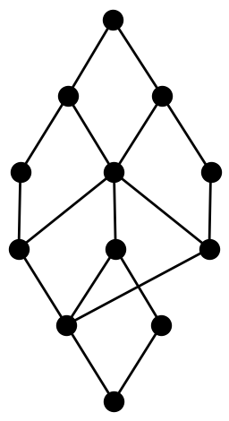
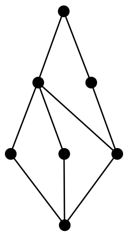
The symmetry types are illustrated in Figure 1. If we take the BF example as the lower summand, and the MC example as the upper summand, we obtain two nonisomorphic vertical 2-sums (both of type CS) as shown in Figure 2.

Note that in an MX piece atoms and coatoms can be swapped independently, but in an MH piece only simultaneously; the shapes of the letters X and H are meant as mnemonics for this.

We will form compositions “bottom up”, adding new pieces over pieces or smaller compositions. The following lemma characterizes how many and what kinds of compositions are formed in different cases.

Lemma 2.

If $L$ is a piece or a composition, and $U$ is a piece, then the number and type of their nonisomorphic vertical 2-sums are as follows.

			$U$ type
$L$ type, any of	MF	MA	MC	MX	MH	TF	TS
CF/BF/MF/MA	$2\!\times\!\mathrm{CF}$	$1\!\times\!\mathrm{CF}$	$2\!\times\!\mathrm{CS}$	$1\!\times\!\mathrm{CS}$	$1\!\times\!\mathrm{CF}$	$2\!\times\!\mathrm{CN}$	$1\!\times\!\mathrm{CN}$
CS/BS/MC/MX/MH	$1\!\times\!\mathrm{CF}$	$1\!\times\!\mathrm{CF}$	$1\!\times\!\mathrm{CS}$	$1\!\times\!\mathrm{CS}$	$1\!\times\!\mathrm{CS}$	$1\!\times\!\mathrm{CN}$	$1\!\times\!\mathrm{CN}$
CN/TF/TS	none	none	none	none	none	none	none

Proof.

Let us first prove the numbers. We proceed by the rows.

Row 1: $L$ has two fixed coatoms. By Lemma 1, if $U$ has fixed atoms (MF, MC or TF), then there are two nonisomorphic vertical 2-sums; otherwise there is one.

Row 2: $L$ has two symmetric coatoms. By Lemma 1 there is one vertical 2-sum up to isomorphism.

Row 3: $L$ has three or more coatoms, so no vertical 2-sums are formed.

Next we deduce the symmetry type of each vertical 2-sum $S_{i}$ ( $i=1,2$ ). We proceed by the columns.

If $U$ is MF or MA, it has fixed coatoms. Then $S_{i}$ cannot have an automorphism that swaps the coatoms of $S_{i}$ , because its restriction to $U$ would be an automorphism that swaps the coatoms of $U$ . Thus $S_{i}$ has fixed coatoms.

If $U$ is MC or MX, it has an automorphism that swaps its coatoms and fixes its atoms; extending with the identity mapping in $L$ gives, in each $S_{i}$ , an automorphism that swaps the coatoms. Thus $S_{i}$ has symmetric coatoms.

If $U$ is MH, then an automorphism of $S_{i}$ that swaps the coatoms also swaps the atoms of $U$ , which are also the coatoms of $L$ . Thus $S_{i}$ has symmetric coatoms if and only if $L$ has symmetric coatoms.

If $U$ is TF or TS, then $S_{i}$ has three or more coatoms and is of type CN. ∎

3. Cartesian counting in a lattice family

In this section we present our main result, a recurrence relation that counts all nonisomorphic compositions in some desired lattice family, provided that the family has suitable form. We also give examples of such families.

Definition 9.

A family $\mathcal{F}$ of graded vi-lattices is (vertically) 2-summable if the following conditions hold:

(C1)

If $L,U\in\mathcal{F}$ and $S$ is one of their vertical 2-sums, then $S\in\mathcal{F}$ .
(C2)

If $S\in\mathcal{F}$ is a vertical 2-sum of $L$ and $U$ , then $L,U\in F$ .

The first condition ensures that vertical 2-sums stay in the family, and the second ensures that all compositions in $\mathcal{F}$ are indeed obtained as vertical 2-sums of smaller lattices in $\mathcal{F}$ .

Theorem 1.

Let $\mathcal{F}$ be a 2-summable family, and let $\mathrm{XX}_{n}$ denote the number of nonisomorphic $n$ -element lattices in $\mathcal{F}$ having symmetry type XX. Then for $n<8$ we have $\mathrm{CF}_{n}=\mathrm{CS}_{n}=\mathrm{CN}_{n}=0$ , and for $n\geq 8$ the following recurrences hold:

	$\displaystyle\mathrm{CF}_{n}$	$\displaystyle=\sum_{j=6}^{n-2}\Big(\mathrm{LF}_{j}\cdot(2\cdot\mathrm{MF}_{k}+\mathrm{MA}_{k}+\mathrm{MH}_{k})\;+\;\mathrm{LS}_{j}\cdot(\mathrm{MF}_{k}+\mathrm{MA}_{k})\Big)$
	$\displaystyle\mathrm{CS}_{n}$	$\displaystyle=\sum_{j=6}^{n-2}\Big(\mathrm{LF}_{j}\cdot(2\cdot\mathrm{MC}_{k}+\mathrm{MX}_{k})\;+\;\mathrm{LS}_{j}\cdot(\mathrm{MC}_{k}+\mathrm{MX}_{k}+\mathrm{MH}_{k})\Big)$
	$\displaystyle\mathrm{CN}_{n}$	$\displaystyle=\sum_{j=6}^{n-2}\Big(\mathrm{LF}_{j}\cdot(2\cdot\mathrm{TF}_{k}+\mathrm{TS}_{k})\;+\;\mathrm{LS}_{j}\cdot(\mathrm{TF}_{k}+\mathrm{TS}_{k})$
where $k=n-j+4$ , and
	$\displaystyle\mathrm{LF}_{j}$	$\displaystyle=\mathrm{CF}_{j}+\mathrm{BF}_{j}+\mathrm{MF}_{j}+\mathrm{MA}_{j}$
	$\displaystyle\mathrm{LS}_{j}$	$\displaystyle=\mathrm{CS}_{j}+\mathrm{BS}_{j}+\mathrm{MC}_{j}+\mathrm{MX}_{j}+\mathrm{MH}_{j}.$

Proof.

For $n<8$ the numbers are zero, because a composition cannot have fewer than $8$ elements.

Let then $n\geq 8$ and consider an $n$ -element CF-type composition $S\in\mathcal{F}$ . There is exactly one way of expressing $S$ as a vertical 2-sum of two lattices $L,U$ such that $U$ is a piece. This $U$ contains the elements of $S$ above and including its highest-ranked neck, plus an augmented bottom element. By condition (C2) we have $L,U\in\mathcal{F}$ . Furthermore, because $|U|\geq 6$ and and $|L|+|U|-4=n$ , it follows that $|L|\leq n-2$ .

We also observe that different nonisomorphic choices of $L$ and $U$ , where $U$ is a piece, lead to nonisomorphic results. To be more precise: If $L\ncong L^{\prime}$ or $U\ncong U^{\prime}$ , and $U$ and $U^{\prime}$ are pieces, then the vertical 2-sums of $L$ and $U$ are not isomorphic to the vertical 2-sums of $L^{\prime}$ and $U^{\prime}$ .

All nonisomorphic $n$ -element CF-type compositions in $\mathcal{F}$ can be counted by considering (for all $j=6,\ldots,n-2$ ) first the choices of a $j$ -element lower summand $L\in\mathcal{F}$ , and then the choices of an upper summand $U\in\mathcal{F}$ such that $U$ is a piece with $k=n-j+4$ elements, subject to the requirement that the resulting vertical 2-sums are of type CF.

Now $\mathrm{LF}_{j}$ is the number of nonisomorphic lower summands that have fixed coatoms. For each such lower summand, by collecting the CF-type results from the first row of the table in Lemma 2, we get $2\cdot\mathrm{MF}_{k}+\mathrm{MA}_{k}+\mathrm{MH}_{k}$ nonisomorphic vertical 2-sums, which are in $\mathcal{F}$ by condition (C1).

Similarly, $\mathrm{LS}_{j}$ is the number of nonisomorphic lower summands that have symmetric coatoms. For each such lower summand, by collecting the CF-type results from the second row of the table in Lemma 2, we get $\mathrm{MF}_{k}+\mathrm{MA}_{k}$ nonisomorphic vertical 2-sums, which are in $\mathcal{F}$ by condition (C1).

Adding up the cases we obtain the stated expression for $\mathrm{CF}_{n}$ . The expressions for $\mathrm{CS}_{n}$ and $\mathrm{CN}_{n}$ follow in the same manner. ∎

Not all families of graded vi-lattices are 2-summable. For a simple example, finite graded rank-four vi-lattices fail both conditions (C1) and (C2). Interestingly, finite geometric lattices are 2-summable but in a vacuous way.

Theorem 2.

The only finite geometric lattice that has a two-element level is $M_{2}$ .

Proof.

Let $L$ be a finite geometric lattice that has a two-element level $\{a,b\}$ . Because $L$ is atomistic, neither $a$ or $b$ has any join-irreducible covers, thus $a$ and $b$ are covered by exactly one element $c$ . Further, because $L$ is necessarily vertically indecomposable, it follows that $c=1_{L}$ , and $a,b$ are the coatoms.

The numbers of atoms and coatoms in a finite geometric lattice of rank $r$ are known as the Whitney numbers $W_{1}$ and $W_{r-1}$ . It is known that $W_{1}\leq W_{r-1}$ ; see e.g. Dowling and Wilson [3]. This implies that our $L$ has two atoms. But we have shown that $L$ cannot have two-element levels other than the coatoms; thus the atoms are the coatoms, and $L=M_{2}$ . ∎

In other words, Theorem 2 says that all finite geometric lattices are special; there are no pieces and no compositions, so no use for the vertical 2-sum. Modular and distributive lattices will be more interesting for our purposes. We first prove an auxiliary result by elementary means.

Lemma 3.

In the Hasse diagram of a finite semimodular lattice, the subgraph induced by two consecutive levels is connected.

Proof.

Let $L$ be a finite semimodular lattice, $L_{k}$ its $k$ th level, and $H_{k}$ the subgraph induced by $L_{k}$ and $L_{k+1}$ . We use induction on $k$ . Clearly $H_{0}$ is connected. Assume then that $H_{k-1}$ is connected. If $L_{k}$ is a singleton, then obviously $H_{k}$ is connected. Otherwise, let $(U,V)$ be any partition of $L_{k}$ into two nonempty subsets. Because $H_{k-1}$ is connected, there is an element in $L_{k-1}$ that is covered by some two elements $u\in U$ and $v\in V$ . Then by semimodularity $u$ and $v$ are covered by some $w\in L_{k+1}$ , so there is a path from $U$ to $V$ in $H_{k}$ . Finally, from every element in $L_{k+1}$ there is an edge to $L_{k}$ . Thus $H_{k}$ is connected. ∎

Note that Lemma 3 also follows from previously known, more general results: Björner [1] proved that finite semimodular lattices are lexicographically shellable, and Collins [2] proved that graded lexicographically shellable lattices are rank-connected (i.e. the subgraph induced by two consecutive levels is connected).

Lemma 4.

The family of finite semimodular vi-lattices is 2-summable.

Proof.

We use subscripted symbols $\wedge_{L}$ , $\vee_{L}$ and $\prec_{L}$ to denote meet, join and covered-by in lattice $L$ .

(C1)

Let $L$ and $U$ be finite semimodular vi-lattices, $S$ their vertical 2-sum, and $N$ the two identified elements of $L$ and $U$ . Clearly $S$ is a vi-lattice. We show that $S$ is semimodular by using Birkhoff’s condition [6, p. 331]. Let $a,b\in S$ such that they cover $a\wedge_{S}b$ . Then $a$ and $b$ have the same rank, and are either below $N$ , in $N$ or above $N$ . If $a,b$ are below $N$ , then because $L$ is semimodular, $a,b\prec_{S}a\vee_{L}b=a\vee_{S}b$ . If $a,b$ are in or above $N$ , then because $U$ is semimodular, $a,b\prec_{S}a\vee_{U}b=a\vee_{S}b$ .
(C2)

Let $S$ be a finite semimodular vi-lattice that is a vertical 2-sum of $L$ and $U$ . Clearly $L$ and $U$ are vi-lattices. We show that they are semimodular, again using Birkhoff’s condition.

First let $a,b\in L$ such that they cover $a\wedge_{L}b$ . If $a,b$ are not the coatoms of $L$ , then $a\vee_{L}b=a\vee_{S}b$ . If $a,b$ are the coatoms of $L$ , then $a\vee_{L}b=1_{L}$ . In both cases $a,b\prec_{L}a\vee_{L}b$ . Thus $L$ is semimodular.

Let then $a,b\in U$ such that they cover $a\wedge_{U}b$ . If $a,b$ are not the atoms of $U$ , then $a\wedge_{U}b=a\wedge_{S}b$ , and because $S$ is semimodular, $a,b\prec_{U}a\vee_{U}b=a\vee_{S}b$ . If $a,b$ are the atoms of $U$ , then they are a neck of $S$ . Because $S$ is semimodular, it follows from Lemma 3 that $a,b$ have a common upper cover $c$ in $S$ . Then also $a,b\prec_{U}c$ . Thus $U$ is semimodular. ∎

Lemma 5.

The family of finite modular vi-lattices is 2-summable.

Proof.

Follows from Lemma 4 by duality. ∎

Lemma 6.

The family of finite distributive vi-lattices is 2-summable.

Proof.

We recall that a finite modular lattice is distributive if and only if it does not contain a cover-preserving diamond [6, p. 109], that is, five distinct elements $o,a,b,c,i$ such that $o\prec a,b,c\prec i$ .

(C1)

Let $L$ and $U$ be finite distributive vi-lattices and $S$ their vertical 2-sum. By Lemma 5 $S$ is modular. Since $L$ and $U$ do not contain a cover-preserving diamond, the only possibility for $S$ to contain one would be with $o\in L$ and $i\in U$ , but the neck consisting of the two identified elements of $L$ and $U$ cannot contain three distinct elements $a,b,c$ . Thus $S$ is distributive.
(C2)

Let $S$ be a finite distributive vi-lattice that is a vertical 2-sum of $L$ and $U$ . By Lemma 5 $L$ and $U$ are modular vi-lattices. Since $S$ does not contain a cover-preserving diamond, the only possibility for $L$ to contain one would be with $i=1_{L}$ , but this is impossible because $L$ has only two coatoms. Thus $L$ is distributive. The case of $U$ is similar. ∎

4. Computations

4.1. Method of classifying a lattice

Given a graded vi-lattice represented by its covering graph, a short piece of program code classifies the lattice into the types described in Section 2. Calculating lattice length, counting atoms and coatoms, and finding possible necks is straightforward. For analyzing the symmetry type we use the Nauty library, version 2.7r1 [14, 15].

Nauty returns the automorphism group of a given directed graph as a list of generators $(\gamma_{1},\ldots,\gamma_{k})$ . To classify a bottom piece we check if any generator swaps the coatoms; in that case the coatoms are symmetric, otherwise fixed. With a top piece we check if any generator swaps the atoms.

To classify a middle piece some more cases are required. For each generator, we check if it:

(A)

swaps the atoms and fixes the coatoms; or
(B)

swaps both the atoms and the coatoms; or
(C)

swaps the coatoms and fixes the coatoms.

Generators that touch neither atoms nor coatoms are ignored. Then:

(1)

If there are no generators of types A/B/C, the piece is MF.
(2)

If there are generators of type A, but none of B/C, the piece is MA.
(3)

If there are generators of type C, but none of A/B, the piece is MC.
(4)

If there are generators of type B, but none of A/C, the piece is MH.
(5)

If there are generators of at least two of the types A/B/C, the piece is MX.

It is easily seen that this procedure produces the correct classification. Note that for an MX piece, Nauty does not necessarily return generators of types A and C. It can instead return, for example, a generator $\gamma_{i}$ of type A, and a generator $\gamma_{j}$ of type B. But then $\gamma_{i}\circ\gamma_{j}$ is an automorphism that swaps the coatoms and fixes the atoms, and then we know that the piece is indeed MX.

4.2. Modular lattices

Modular vi-lattices were previously generated and counted up to 30 elements in [12], and up to 33 elements in unpublished work [16]. That was done with a program that starts from length-two seed lattices, and then adds new levels of elements recursively. The program lists exactly one representative lattice from each isomorphism class.

We use here essentially the same lattice-generating program, modified so that it skips all compositions, and generates only the pieces and the specials. The modification is simply that two-element levels are not allowed between coatom and atom levels, because such a level would form a neck.

With this program, all modular pieces and specials of $n\leq 35$ elements were generated (up to isomorphism), and classified as described in §4.1. Because modular vi-lattices are 2-summable (Lemma 5), the numbers of modular compositions of $n\leq 35$ elements are then calculated using Theorem 1.

The results of the exact counting are shown in Table 1. Rows MF–TF and “special” are from direct counting with the lattice-generating program. Rows CF–CN are calculated with the recurrence in Theorem 1. Row “vi-latt.” contains the numbers of all modular vi-lattices: this is the sum of specials, pieces and compositions. Finally, row “all” has the numbers of all modular lattices (including vertical sums of vi-lattices), calculated with the vertical sum recurrence (1).

An exponential lower bound is derived as follows. Using Theorem 1 with the known numbers of modular pieces of up to 35 elements, and plugging in zeros for larger pieces (whose numbers we do not know), we obtain lower bounds on $\mathrm{CF}_{n}$ , $\mathrm{CS}_{n}$ and $\mathrm{CN}_{n}$ for $n$ arbitrarily large. We observe that the growth ratios (from $n$ to $n+1$ ) of all three lower bounds settle a little above 2.3122 for $n$ large enough. To obtain rigorous lower bounds, we choose a convenient starting point $n=50$ , convenient constant coefficients in front, and apply induction.

Theorem 3.

The numbers of nonisomorphic modular compositions of types CF, CS and CN have the following lower bounds, when $n\geq 50$ :

	$\displaystyle\mathrm{CF}_{n}$	$\displaystyle\geq 0.002910\times 2.3122^{n}$
	$\displaystyle\mathrm{CS}_{n}$	$\displaystyle\geq 0.000035\times 2.3122^{n}$
	$\displaystyle\mathrm{CN}_{n}$	$\displaystyle\geq 0.002470\times 2.3122^{n}$

Proof.

For $50\leq n\leq 85$ the claim follows by direct calculation with Theorem 1, using the numbers of pieces from Table 1, and zeros when the number of pieces is not known.

For $n>85$ the claim follows by induction on $n$ . Let $n>85$ be arbitrary, and assume that the claimed lower bounds hold on $\mathrm{CF}_{m}$ , $\mathrm{CS}_{m}$ and $\mathrm{CN}_{m}$ when $n-35\leq m\leq n-1$ . Then applying Theorem 1 gives the claimed lower bounds on $\mathrm{CF}_{n}$ , $\mathrm{CS}_{n}$ and $\mathrm{CN}_{n}$ , which completes the induction. ∎

Corollary 1.

There are at least $0.005415\times 2.3122^{n}$ nonisomorphic modular vi-lattices of $n$ elements when $n\geq 50$ .

Proof.

Add up the three lower bounds from Theorem 3. ∎

Corollary 2.

There are at least $0.02\times 2.3713^{n}$ nonisomorphic modular lattices of $n$ elements when $n\geq 100$ .

Proof.

For $100\leq n\leq 400$ the claim follows by direct calculation with recurrence (1), using as input the lower bounds on vi-lattices of up to $400$ elements computed using Theorem 3.

For the induction step, let $n>400$ be arbitrary, and assume that the claimed lower bound holds for the previous $300$ values. Applying (1) then gives the claimed lower bound for the number of $n$ -element modular lattices. This completes the induction. ∎

4.3. Distributive lattices

Distributive vi-lattices were previously counted up to 49 elements by Erné et al. [4, 17]. To count $n$ -element distributive lattices, they actually generated posets that have $n$ antichains; these are in a bijective correspondence with the distributive lattices.

Our approach is more direct. We generate the distributive lattices directly, using the same program that we used for modular lattices, with some modifications. The first modification is a condition that ensures that we generate only the distributive lattices. Since the original program generates modular lattices, we only need to check that whenever a new element is created, it does not create a cover-preserving diamond [6, p. 109]. This ensures that we generate the distributive lattices but no others.

We also employ an important optimization that cuts short search branches that cannot lead to distributive lattices. Our lattice-generating program (see [12] for more details) builds lattices levelwise, top down, until the number of elements reaches a preset maximum. When creating a new level, it adds new elements in decreasing order of updegree. The last step on each level is thus to create meet-irreducible elements. In the original algorithm, this step can create a large number of meet-irreducible elements, limited only by the maximum lattice size. But in a distributive lattice we can limit their number as follows. We recall (see Corollary 112 in [6]) that the number of meet-irreducible elements in a distributive lattice equals the lattice length. As we build a lattice, we keep track of the meet-irreducible elements created so far, and at each level we compute an updated upper bound $R$ on the lattice length (based on the current length and the budget of remaining elements). The number of meet-irreducible elements, including the ones already created, is then limited to be at most $R$ .

With this program, all distributive pieces and specials of $n\leq 60$ elements were generated (up to isomorphism), and classified with the method described in §4.1. Compositions were then counted using Theorem 1. The results are shown in Table 2.

An exponential lower bound is derived in the same way as with modulars. Using Theorem 1 with the known numbers of distributive pieces of up to 60 elements, and plugging in zeros for larger pieces, we obtain lower bounds on $\mathrm{CF}_{n}$ , $\mathrm{CS}_{n}$ and $\mathrm{CN}_{n}$ whose growth ratios settle a little above 1.7250 for $n$ large enough. To obtain rigorous lower bounds, we choose a convenient starting point $n=100$ , convenient constant coefficients in front, and apply induction.

Theorem 4.

The numbers of nonisomorphic distributive compositions of types CF, CS and CN have the following lower bounds, when $n\geq 100$ :

	$\displaystyle\mathrm{CF}_{n}$	$\displaystyle\geq 0.010600\times 1.7250^{n}$
	$\displaystyle\mathrm{CS}_{n}$	$\displaystyle\geq 0.000092\times 1.7250^{n}$
	$\displaystyle\mathrm{CN}_{n}$	$\displaystyle\geq 0.001950\times 1.7250^{n}$

Proof.

For $100\leq n\leq 161$ the claim follows by direct calculation with Theorem 1, using the numbers of pieces from Table 2, and zeros when the number of pieces is not known.

For $n>161$ the claim follows by induction on $n$ . Let $n>161$ be arbitrary, and assume that the claimed lower bounds hold on $\mathrm{CF}_{m}$ , $\mathrm{CS}_{m}$ and $\mathrm{CN}_{m}$ when $n-61\leq m\leq n-1$ . Then applying Theorem 1 gives the claimed lower bounds on $\mathrm{CF}_{n}$ , $\mathrm{CS}_{n}$ and $\mathrm{CN}_{n}$ , which completes the induction. ∎

Corollary 3.

There are at least $0.012642\times 1.7250^{n}$ nonisomorphic distributive vi-lattices of $n$ elements when $n\geq 100$ .

Proof.

Add up the three lower bounds from Theorem 4. ∎

Corollary 4.

There are at least $0.088\times 1.8433^{n}$ nonisomorphic distributive lattices of $n$ elements when $n\geq 100$ .

Proof.

For $100\leq n\leq 400$ the claim follows by direct calculation with recurrence (1), using as input the lower bounds on vi-lattices of up to $400$ elements computed using Theorem 4.

For the induction step, let $n>400$ be arbitrary, and assume that the claimed lower bound holds for the previous $300$ values. Applying (1) then gives the claimed lower bound for the number of $n$ -element distributive lattices. This completes the induction. ∎

4.4. Semimodular lattices

Although semimodular vi-lattices are 2-summable, vertical 2-sum is not very useful with them. For example, of the $1\;753\;185\;150$ semimodular vi-lattices of $25$ elements, only about $23\%$ are compositions. This is in stark contrast with modular and distributive lattices. Basically this is because semimodular lattices are short and wide (cf. Figures 4–5 in [12]). For this reason we do not include tables of semimodular lattices here, but such tables can be easily computed using the accompanying program code.

We could apply the same techniques as above to obtain an exponential lower bound. But an asymptotically stronger lower bound is obtained by constructing semimodular lattices from Steiner triple systems. A Steiner triple system is a set of $k$ elements (points) and a collection of their 3-sets (triples), such that each pair of distinct points occurs in exactly one triple. By counting the pairs it is easily seen that the number of triples must be $k(k-1)/6$ . It is known that Steiner triple systems on $k$ points exist if and only if $k\equiv 1\text{ or }3\pmod{6}$ ; such values of $k$ are called admissible.

Given a Steiner triple system on $k\geq 7$ points, if we take the points as atoms, the triples as coatoms, and augment a top and a bottom, we obtain a rank-three semimodular vi-lattice, because each pair of atoms is covered by exactly one coatom. The lattice has $k+k(k-1)/6+2$ elements.

Theorem 5.

For any $n\geq 100$ , the number of nonisomorphic semimodular rank-three vi-lattices containing $n$ elements is at least

\big(0.3286\;n^{1/8}\big)^{n}.

Proof.

Let $n\geq 100$ be given. Choose the largest admissible $k$ such that

k+k(k-1)/6+2\leq n.

Then $k\geq 21$ , and because admissible values are at most 4 units apart, we have

(2)

n<(k+4)+(k+4)(k+3)/6+2<k^{2}/3.

Let $N$ be the number of nonisomorphic Steiner triple systems on $k$ points. By Wilson’s Theorem 2 [18], we have

N\geq(e^{-5}k)^{k^{2}/12},

and using the bound $k>\sqrt{3n}$ from (2) we obtain

N\geq\big(e^{-5}\cdot\sqrt{3n}\big)^{n/4}=\big(e^{-5/4}\cdot 3^{1/8}\cdot n^{1/8}\big)^{n}\geq\big(0.3286\;n^{1/8}\big)^{n}.

From these $N$ Steiner triple systems on $k$ points, we can form $N$ nonisomorphic semimodular rank-three vi-lattices that have $n^{\prime}=k+k(k-1)/6+2$ elements, and by our choice of $k$ , we have $n^{\prime}\leq n$ . To each lattice, add $n-n^{\prime}$ extra coatoms covering an arbitrarily chosen atom of the highest updegree. This operation makes the lattices have exactly $n$ elements, and preserves semimodularity and nonisomorphism, so the claim follows. ∎

The lower bound in Theorem 5 is very loose (it does not even exceed $1$ until $n\approx 7000$ ), and is presented in simple terms just to demonstrate the asymptotic behaviour, that the number of semimodular vi-lattices grows faster than any exponential in $n$ . The bound might be improved in several ways, for example, by using Keevash’s recent improvement on Wilson’s lower bound [9].

4.5. Notes on computation

The main computational load was in generating the pieces and specials. For the largest sizes this was parallelized by running the lattice-generating program until a predefined number of elements had been added. The search state at those points was saved to a file, and the remaining work was divided among worker processes. For modular lattices of $33$ , $34$ and $35$ elements, this computation took $8.9$ , $23.7$ and $63.1$ cpu-core-days on Intel Xeon Gold 6230 processors (nominally 2.1 GHz). The time grows roughly $2.66$ -fold as $n$ grows by one. For distributive lattices of $58$ , $59$ and $60$ elements, the computation took $6.3$ , $10.4$ and $17.2$ cpu-core-days, growing roughly $1.66$ -fold each time.

The optimization in §4.3 that made it possible to count distributive lattices up to $60$ elements is just one example, out of many, where the speed of a combinatorial search is greatly affected by a simple, innocent-looking bounding condition. Here its implementation takes about a dozen lines of code (see the accompanying program code for details). But already at $30$ elements, it speeds up the generation of distributive pieces and specials from 153 seconds to 0.4 seconds; and the savings ratio keeps improving as the lattices grow.

Unfortunately, it is not always easy to come up with conditions that actually have a great impact, and are also fast enough to compute during the search. Given the large existing theory of the structure of distributive and modular lattices, it is conceivable that our lattice-generating program could still be much improved by imposing some other, so far untried, bounding conditions.

4.6. Partial verification

We describe here some of the methods that were used to partially verify the correctness of the computational results.

The pieces and specials were generated and classified twice, on different computers. The counts and the actual lattice listings were verified to be identical by comparing their MD5 checksums. This would help against transient hardware and operational errors, but not against systematic errors in the program the.

The number of MA pieces equals the number of MC pieces in each column of Tables 1 and 2. This is as it should, because such pieces are duals of each other. The same holds between BF and TF pieces, and between BS and TS pieces.

We also performed a more thorough duality check. The rank sequence of a graded lattice is the sequence of its level sizes from bottom to top. The rank sequences of a lattice and its dual are reverses of each other. In Figure 1 the BF example piece has rank sequence $(1,3,2,1)$ , and its dual, the TF example piece has $(1,2,3,1)$ . We counted the occurrences of each combination of symmetry type and rank sequence in pieces and specials, and verified that the numbers match between the dual pairs (MF–MF, MA–MC, MX–MX, MH–MH, BF–TF, BS–TF, and special–special). For example, among all $60$ -element distributive MX pieces, there are $2\;137$ whose rank sequence is $(1,2,3,4,6,5,4,4,4,4,4,4,3,3,3,3,2,1)$ , and $2\;137$ whose sequence is its reverse. If any of the lattice listings were accidentally truncated or corrupted, this would likely be detected as a mismatch. An error in the lattice-generating logic or in the classification code would also have a good chance of causing a mismatch.

As a consistency check of the Cartesian counting logic, we directly generated, classified and counted all distributive vi-lattices of 50 elements including compositions. In each class, the count thus obtained matches the calculated count in Table 2. Generating these 50-element lattices took $12.6$ cpu-core-days, about 70 times longer than with compositions excluded, which also demonstrates the benefits of Cartesian counting.

Our totals on rows “vi-latt.” and “all” agree with previously published numbers of modular lattices to 33 elements [12, 16] and distributive lattices to 49 elements [4] (except at $n=1$ , because we count the singleton as a vi-lattice). The previous countings did not employ the vertical 2-sum.

5. Concluding remarks

One of our stated goals was to create more compact lattice listings by leaving out all compositions (vertical 2-sums of smaller lattices). As seen in Tables 1 and 2, this was more successful with distributive lattices than with modulars. Compositions make up $79\%$ of the modular vi-lattices of $35$ elements, and $99.6\%$ of the distributive vi-lattices of $60$ elements.

The observed growths of the numbers of modular and distributive vi-lattices, to the extent that they are now known, are illustrated in Figure 3. In modular vi-lattices our lower bound $\Omega(2.3122^{n})$ seems loose; the observed ratios keep increasing, hinting perhaps of a (very slightly) superexponential growth. We note that no exponential upper bound is currently known on the number of modular lattices. In distributive vi-lattices the observed ratios seem to be converging, and our lower bound $\Omega(1.7250^{n})$ seems pretty good.

Figure 3. Ratio between the numbers of nonisomorphic vi-lattices of

(n\!-\!1)

and

n

elements, with and without vertical 2-sums.

Erné et al. have shown an upper bound of $O(2.33^{n})$ on nonisomorphic distributive vi-lattices [4]. Our improved lower bound $\Omega(2.3122^{n})$ on nonisomorphic modular vi-lattices is still not enough to separate the growth rates of these two families. To close the gap there are different options. We could count modular pieces further. Empirically, adding one element increases the base in our lower bound by $0.0048$ (but the increase diminishes as $n$ grows). Counting the pieces up to $40$ elements would probably raise the lower bound above $\Omega(2.33^{n})$ . But this would take about $10\;000$ cpu-core-days with the current lattice-generating program, and was deemed not worth the effort. Improving the algorithm or the lower bound techniques might be a better idea. Another option is to improve the upper bound on distributive vi-lattices. Indeed, Erné et al. note that “with more effort” it might be improved considerably, at least to $2.28^{n}$ . Combined with our lower bound, this would suffice to separate the growth rates.

Although our lower bounds are based on large computations, we must point out that proper analysis of symmetry is the key to good lower bounds. Indeed, using all our data on distributive lattices ( $n\leq 60$ ), if we ignore the symmetry cases (and lose the factors of 2 in Theorem 1), we only obtain a bound of $\Omega(1.6213^{n})$ for distributive vi-lattices. In contrast, using just the distributive middle pieces of $n\leq 21$ elements (a truly modest collection of 134 lattices), our symmetry-distinguishing method already gives $\Omega(1.6818^{n})$ .

Accompanying program code is available in Bitbucket [10]. This includes C programs to generate the pieces and the specials, to classify and count them by symmetry type, and to perform the Cartesian counting. Also included is SageMath code for verifying the exponential lower bounds. The lattice listings (pieces and specials only) were stored in digraph6 format and compressed with xz. The compressed listings take about 167 GB of disk space, and will be available in [11].

Table 1. Number of modular lattice up to isomorphism.

	$n$
type	1	2	3	4	5	6	7	8	9	10	11	12	13	14	15	16
MF	0	0	0	0	0	1	0	0	2	3	3	13	24	48	105	242
MA	0	0	0	0	0	0	0	0	0	0	0	1	1	2	5	7
MC	0	0	0	0	0	0	0	0	0	0	0	1	1	2	5	7
MX	0	0	0	0	0	0	0	0	0	0	0	0	0	0	0	1
MH	0	0	0	0	0	0	0	0	1	0	1	0	1	0	2	2
BF	0	0	0	0	0	0	1	1	1	4	6	11	25	56	113	257
BS	0	0	0	0	0	0	0	0	0	1	1	2	4	5	9	15
TF	0	0	0	0	0	0	1	1	1	4	6	11	25	56	113	257
TS	0	0	0	0	0	0	0	0	0	1	1	2	4	5	9	15
CF	0	0	0	0	0	0	0	2	2	6	16	38	80	208	464	1115
CS	0	0	0	0	0	0	0	0	0	0	0	0	0	3	5	15
CN	0	0	0	0	0	0	0	0	2	4	10	28	66	154	375	884
special	1	1	0	1	1	1	1	3	3	5	10	20	35	75	151	317
pieces	0	0	0	0	0	1	2	2	5	13	18	41	85	174	361	803
compos.	0	0	0	0	0	0	0	2	4	10	26	66	146	365	844	2014
vi-latt.	1	1	0	1	1	2	3	7	12	28	54	127	266	614	1356	3134
all	1	1	1	2	4	8	16	34	72	157	343	766	1718	3899	8898	20475

	$n$
type	17	18	19	20	21	22	23	24
MF	518	1185	2664	6092	13849	31932	73458	170112
MA	15	28	61	122	270	570	1259	2729
MC	15	28	61	122	270	570	1259	2729
MX	1	4	5	11	18	35	63	124
MH	5	8	11	19	22	43	51	105
BF	557	1250	2763	6267	14125	32225	73561	169304
BS	30	52	109	207	422	835	1721	3544
TF	557	1250	2763	6267	14125	32225	73561	169304
TS	30	52	109	207	422	835	1721	3544
CF	2580	6156	14382	34236	80703	192141	455548	1086269
CS	35	84	191	457	1054	2482	5795	13601
CN	2091	4959	11736	27832	66009	156845	372956	888193
special	657	1426	3074	6783	15006	33707	75944	172893
pieces	1728	3857	8546	19314	43523	99270	226654	521495
compos.	4706	11199	26309	62525	147766	351468	834299	1988063
vi-latt.	7091	16482	37929	88622	206295	484445	1136897	2682451
all	47321	110024	256791	601991	1415768	3340847	7904700	18752943

Table 1 (continued). Number of modular lattice up to isomorphism.

	$n$
type	25	26	27	28	29	30
MF	394356	918597	2142885	5016593	11766661	27673169
MA	6054	13395	29981	67308	152290	345897
MC	6054	13395	29981	67308	152290	345897
MX	239	474	945	1911	3917	8094
MH	148	290	454	826	1359	2352
BF	390258	904769	2102583	4905597	11472236	26908706
BS	7475	15902	34379	75030	165752	369140
TF	390258	904769	2102583	4905597	11472236	26908706
TS	7475	15902	34379	75030	165752	369140
CF	2586652	6179943	14763845	35347971	84670699	203133686
CS	31931	75120	176999	417863	988002	2340245
CN	2117276	5054559	12078748	28902161	69228582	166012187
special	395073	908830	2098043	4866320	11320574	26427788
pieces	1202317	2787493	6478170	15115200	35352493	82931101
compos.	4735859	11309622	27019592	64667995	154887283	371486118
vi-latt.	6333249	15005945	35595805	84649515	201560350	480845007
all	44588803	106247120	253644319	606603025	1453029516	3485707007

	$n$
type	31	32	33	34	35
MF	65203834	153963391	364151886	862779754	2047145114
MA	790496	1813615	4180886	9673363	22467366
MC	790496	1813615	4180886	9673363	22467366
MX	16975	35876	76749	165615	360878
MH	3958	6696	11466	19465	33807
BF	63245392	148991342	351620380	831365583	1968780807
BS	829576	1877307	4277558	9800078	22571155
TF	63245392	148991342	351620380	831365583	1968780807
TS	829576	1877307	4277558	9800078	22571155
CF	487682310	1172237243	2819860668	6789965627	16361898245
CS	5551716	13191092	31388574	74798062	178482514
CN	398494238	957517799	2302844911	5543373958	13354884177
special	61853133	145160950	341431589	804878006	1901058538
pieces	194955695	459370491	1084397749	2564642882	6075178455
compos.	891728264	2142946134	5154094153	12408137647	29895264936
vi-latt.	1148537092	2747477575	6579923491	15777658535	37871501929
all	8373273835	20139498217	48496079939	116905715114	282098869730

Table 2. Number of distributive lattices up to isomorphism.

	$n$
type	1	2	3	4	5	6	7	8	9	10	11	12	13	14	15	16	17
MF	0	0	0	0	0	1	0	0	0	0	0	3	0	0	4	5	4
MA	0	0	0	0	0	0	0	0	0	0	0	0	0	0	1	0	0
MC	0	0	0	0	0	0	0	0	0	0	0	0	0	0	1	0	0
MX	0	0	0	0	0	0	0	0	0	0	0	0	0	0	0	0	0
MH	0	0	0	0	0	0	0	0	1	0	0	0	0	0	0	1	0
BF	0	0	0	0	0	0	0	0	0	1	0	0	0	2	1	3	1
BS	0	0	0	0	0	0	0	0	0	0	0	0	1	0	0	0	1
TF	0	0	0	0	0	0	0	0	0	1	0	0	0	2	1	3	1
TS	0	0	0	0	0	0	0	0	0	0	0	0	1	0	0	0	1
CF	0	0	0	0	0	0	0	2	0	4	2	10	6	32	18	83	74
CS	0	0	0	0	0	0	0	0	0	0	0	0	0	1	0	0	2
CN	0	0	0	0	0	0	0	0	0	0	0	2	0	4	2	14	8
special	1	1	0	1	0	0	0	1	0	0	0	1	0	1	0	3	1
pieces	0	0	0	0	0	1	0	0	1	2	0	3	2	4	8	12	8
compos.	0	0	0	0	0	0	0	2	0	4	2	12	6	37	20	97	84
vi-latt.	1	1	0	1	0	1	0	3	1	6	2	16	8	42	28	112	93
all	1	1	1	2	3	5	8	15	26	47	82	151	269	494	891	1639	2978

	$n$
type	18	19	20	21	22	23	24	25	26
MF	16	10	29	49	63	94	213	219	459
MA	0	1	1	2	1	3	3	10	8
MC	0	1	1	2	1	3	3	10	8
MX	0	0	0	0	0	0	1	0	1
MH	1	0	0	0	1	1	0	3	2
BF	8	7	16	16	40	38	102	116	229
BS	0	1	1	2	1	5	2	8	4
TF	8	7	16	16	40	38	102	116	229
TS	0	1	1	2	1	5	2	8	4
CF	230	233	672	726	1928	2342	5516	7280	16178
CS	1	5	2	14	9	37	27	99	95
CN	41	27	120	104	343	347	1005	1119	2953
special	6	2	10	6	26	18	56	48	131
pieces	33	28	65	89	148	187	428	490	944
compos.	272	265	794	844	2280	2726	6548	8498	19226
vi-latt.	311	295	869	939	2454	2931	7032	9036	20301
all	5483	10006	18428	33749	62162	114083	210189	386292	711811

Table 2 (continued). Number of distributive lattices up to isomorphism.

	$n$
type	27	28	29	30	31	32	33
MF	726	1099	1691	3112	4176	7573	11728
MA	15	14	50	47	87	121	227
MC	15	14	50	47	87	121	227
MX	0	2	0	4	3	5	4
MH	1	2	2	8	2	10	6
BF	303	596	749	1513	2033	3647	5316
BS	16	11	32	25	59	62	151
TF	303	596	749	1513	2033	3647	5316
TS	16	11	32	25	59	62	151
CF	22302	47348	68582	138752	208961	409676	632745
CS	281	301	789	926	2307	2865	6611
CN	3594	8607	11348	25363	35198	74935	108658
special	129	328	339	769	914	1913	2371
pieces	1395	2345	3355	6294	8539	15248	23126
compos.	26177	56256	80719	165041	246466	487476	748014
vi-latt.	27701	58929	84413	172104	255919	504637	773511
all	1309475	2413144	4442221	8186962	15077454	27789108	51193086

	$n$
type	34	35	36	37	38	39
MF	18593	29332	49894	73906	125464	196346
MA	279	584	732	1333	1963	3362
MC	279	584	732	1333	1963	3362
MX	18	15	20	22	71	68
MH	16	9	16	26	31	40
BF	9431	13450	24024	35267	60195	91542
BS	147	317	369	755	927	1833
TF	9431	13450	24024	35267	60195	91542
TS	147	317	369	755	927	1833
CF	1211099	1914417	3583636	5772993	10632469	17361550
CS	8863	19257	27094	56362	82534	165301
CN	221306	333256	655975	1014990	1947706	3081099
special	4783	6192	11888	16279	29902	42083
pieces	38341	58058	100180	148664	251736	389928
compos.	1441268	2266930	4266705	6844345	12662709	20607950
vi-latt.	1484392	2331180	4378773	7009288	12944347	21039961
all	94357143	173859936	320462062	590555664	1088548290	2006193418

Table 2 (continued). Number of distributive lattices up to isomorphism.

	$n$
type	40	41	42	43	44
MF	316251	501232	824706	1277065	2104201
MA	4763	8706	12369	21206	32381
MC	4763	8706	12369	21206	32381
MX	137	132	314	389	739
MH	39	72	82	100	131
BF	154501	234005	395667	606372	1005172
BS	2286	4424	5957	10857	15117
TF	154501	234005	395667	606372	1005172
TS	2286	4424	5957	10857	15117
CF	31576370	52152822	93836823	156430892	279134095
CS	250864	486894	758311	1439247	2287530
CN	5786183	9323041	17211623	28123776	51240833
special	75946	109160	191940	283583	488243
pieces	639527	995706	1653088	2554424	4210411
compos.	37613417	61962757	111806757	185993915	332662458
vi-latt.	38328890	63067623	113651785	188831922	337361112
all	3697997558	6815841849	12563729268	23157428823	42686759863

	$n$
type	45	46	47	48
MF	3324318	5359557	8530466	13845649
MA	54061	81642	139008	210288
MC	54061	81642	139008	210288
MX	858	1710	2298	4073
MH	157	263	252	415
BF	1566178	2579549	4019531	6615167
BS	27265	38591	68176	99857
TF	1566178	2579549	4019531	6615167
TS	27265	38591	68176	99857
CF	468610361	830767951	1402696804	2473422299
CS	4259645	6888356	12629975	20697992
CN	84668721	152604200	254469592	454703002
special	731917	1246418	1890209	3178981
pieces	6620341	10761094	16986446	27700761
compos.	557538727	990260507	1669796371	2948823293
vi-latt.	564890985	1002268019	1688673026	2979703035
all	78682454720	145038561665	267348052028	492815778109

Table 2 (continued). Number of distributive lattices up to isomorphism.

	$n$
type	49	50	51	52
MF	21848698	35484402	56423044	90846703
MA	349946	545640	894103	1392365
MC	349946	545640	894103	1392365
MX	5652	10074	14075	24970
MH	440	697	770	1034
BF	10365640	16917992	26705669	43421020
BS	171474	256172	436542	657562
TF	10365640	16917992	26705669	43421020
TS	171474	256172	436542	657562
CF	4195545640	7366918781	12541052681	21947209314
CS	37503756	62106875	111453001	186162978
CN	763638695	1355285715	2289013709	4040233169
special	4883596	8125938	12584095	20810796
pieces	43628910	70934781	112510517	181814601
compos.	4996688091	8784311371	14941519391	26173605461
vi-latt.	5045200597	8863372090	15066614003	26376230858
all	908414736485	1674530991462	3086717505436	5689930182502

	$n$
type	53	54	55	56
MF	144993779	233835914	372140014	600341635
MA	2298377	3582354	5856047	9243133
MC	2298377	3582354	5856047	9243133
MX	35929	61578	91665	155593
MH	1401	1762	2365	2920
BF	68622251	111467609	176619879	285832100
BS	1108440	1696359	2822398	4362272
TF	68622251	111467609	176619879	285832100
TS	1108440	1696359	2822398	4362272
CF	37469608053	65395110178	111905017483	194884875094
CS	331472539	557422364	986467033	1667764379
CN	6854924656	12046207362	20511977357	35920244327
special	32424737	53285185	83549296	136565579
pieces	289089245	467391898	742830692	1199375158
compos.	44656005248	77998739904	133403461873	232472883800
vi-latt.	44977519230	78519416987	134229841861	233808824537
all	10488501786986	19334113091637	35639590512519	65696773057331

Table 2 (continued). Number of distributive lattices up to isomorphism.

	$n$
type	57	58	59	60
MF	958148836	1540236160	2462775718	3959945640
MA	15005164	23705048	38546064	60946820
MC	15005164	23705048	38546064	60946820
MX	231975	392608	596474	990499
MH	3980	5148	6470	8675
BF	454454916	733959291	1168085737	1885053587
BS	7218116	11214722	18454173	28883114
TF	454454916	733959291	1168085737	1885053587
TS	7218116	11214722	18454173	28883114
CF	334097123844	580839511384	997199063829	1731270488614
CS	2936919383	4986729668	8746804291	14902405273
CN	61338845389	107114456244	183330850349	319426226966
special	215048026	350313997	553415624	898644768
pieces	1911741183	3078392038	4913550610	7910711856
compos.	398372888616	692940697296	1189276718469	2065599120853
vi-latt.	400499677825	696369403331	1194743684703	2074408477477
all	121102696325898	223236665889804	411506035223499	758556959660012

Acknowledgments

Computational resources were provided by CSC – IT Center for Science and by the Aalto Science-IT project.

References

[1] Anders Björner. Shellable and Cohen-Macaulay partially ordered sets. Transactions of the American Mathematical Society, 260:159–183, 1980.
[2] Karen L. Collins. Planar lattices are lexicographically shellable. Order, 8:375–381, 1992.
[3] Thomas A. Dowling and Richard M. Wilson. Whitney number inequalities for geometric lattices. Proceedings of the American Mathematical Society, 47:504–512, 1975.
[4] Marcel Erné, Jobst Heitzig, and Jürgen Reinhold. On the number of distributive lattices. The Electronic Journal of Combinatorics, 9:Article #R24, 2002.
[5] Volker Gebhardt and Stephen Tawn. Constructing unlabelled lattices. Journal of Algebra, 545:213–236, 2020.
[6] George Grätzer. Lattice Theory: Foundation. Birkhäuser, Basel, 2011.
[7] Jobst Heitzig and Jürgen Reinhold. Counting finite lattices. Algebra universalis, 48:43–53, 2002.
[8] Peter Jipsen and Nathan Lawless. Generating all finite modular lattices of a given size. Algebra universalis, 74:253–264, 2015.
[9] Peter Keevash. Counting Steiner triple systems. In European Congress of Mathematics, pages 459–481, 2018.
[10] Jukka Kohonen. Cartesian lattice counting. https://bitbucket.org/jkohonen/cartesian-lattice-counting/.
[11] Jukka Kohonen. Modular and distributive lattices without vertical sums and 2-sums. https://b2share.eudat.eu. In preparation.
[12] Jukka Kohonen. Generating modular lattices up to 30 elements. Order, 36:423–435, 2018.
[13] Jukka Kohonen. Exponential lower bounds of lattice counts by vertical sum and 2-sum. Algebra universalis, 80, 2019.
[14] Brendan D. McKay and Adolfo Piperno. Nauty and Traces home page (version 2.7r1). http://pallini.di.uniroma1.it/.
[15] Brendan D. McKay and Adolfo Piperno. Practical graph isomorphism, II. Journal of Symbolic Computation, 60:94–112, 2014.
[16] OEIS, the on-line encyclopedia of integer sequences. https://oeis.org/A006981. Number of unlabeled modular lattices with n elements.
[17] OEIS, the on-line encyclopedia of integer sequences. https://oeis.org/A006982. Number of unlabeled distributive lattices with n elements.
[18] Richard M. Wilson. Nonisomorphic Steiner triple systems. Mathematische Zeitschrift, 135:303–313, 1974.