Feasibility Analysis for the Problem of Active Near Field/Far Field Acoustic Pattern Synthesis in Free Space and Shallow Water Environments

In this section, we present a general description of the active manipulation scheme for Helmholtz fields proposed in our previous works. The unified geometric and functional framework has already been discussed in [32, 26, 50]. We shall briefly recall several essential theoretical results and geometric configurations.

The problem is to characterize an active source (modeled as surface pressure or surface normal velocity) so that its generated field approximate some prescribed fields in several exterior regions of interest while maintaining desired patterns in several given far field directions. In this paper, the active field manipulation scheme is explored in both free space and homogeneous ocean with a constant depth environments. The geometries of the problem in free space and homogeneous ocean are sketched in Fig. 1 and Fig. 2, respectively. Although the theoretical discussion in [32, 26, 50] shows that an arbitrary number of source regions, exterior control regions, and far-field directions can be considered in the active scheme, for exemplification we only consider here a single source $D_{a}$, two control regions $D_{1}$, $D_{2}$, and two far-field directions $\mathbf{x_{1}}$, $\mathbf{x_{2}}$ for illustrative purposes. A single source $D_{a}\Subset\mathbb{R}^{3}$ is modeled as a compact region in both free space and homogeneous ocean. The control regions $D_{1}$ and $D_{2}$ are mutually disjoint smooth domains, i.e., $D_{1}\cap D_{2}=\emptyset$. We assume that the control regions are well-separated from the source region, i.e., $(D_{1}\cup D_{2})\cap D_{a}=\emptyset$. Furthermore, we consider two distinct directions ${\bf x}_{1}$ and ${\bf x}_{2}$ representing the far-field directions of interest.

Mathematically the problem is to find the boundary input on the source, either a Dirichlet input data $p$ (pressure) or a Neumann input data $v_{n}$ (normal velocity) such that for any desired field $f=(f_{1},f_{2})$ on the control regions $D_{1}$, $D_{2}$ and prescribed far field pattern values $f_{\infty}=(f_{\infty,1},f_{\infty,2})$, the solution $u$ of the following exterior Helmholtz problem:

$$\left\{\begin{array}[]{llll}\nabla^{2}u+k^{2}u=0\mbox{ in }\mathbb{R}^{3}\!\setminus D_{a}\vskip 4.26773pt,\\ \nabla u\cdot{\bf n}=v_{n},(\mbox{ or }u=p)\mbox{ on }\partial D_{a},\\ \text{corresponding boundary conditions},\\ \text{suitable radiation condition}\end{array}\right.$$

(1)

satisfies the control constraints

$$\begin{cases}\|u-f_{l}\|_{C^{2}(D_{l})}\leq\mu\text{ for }l=\overline{1,2}\>,\\ |u_{\infty}(\hat{\bf x}_{j})-f_{\infty,j}|\leq\mu\text{ for }j=\overline{1,2}\>,\end{cases}$$

(2)

where $0<\mu\ll 1$ is the desired control accuracy threshold and $u_{\infty}$ denotes the the far field pattern of $u$. In (1) and (2), ${\bf n}$ denotes the outward pointing vector normal to $\partial D_{a}$ and ${\hat{{\bf x}}}=\frac{{\bf x}}{|{\bf x}|}$ is the unit vector along the direction ${\bf x}$. The subscript $C^{2}$ denotes the norm in the space of smooth functions with continuous derivatives up to the second order computed as a sum of the $L^{2}$ norms of all the partial derivatives up to the second order where the $L^{2}$ norm on the space of square integrable functions on a given domain $D$ is defined as $\|f\|^{2}_{L^{2}(D)}=\int_{D}|f(\mathbf{x})|^{2}~d{\mathbf{x}}$. The boundary conditions and radiation condition in (1) are corresponding to the medium (environment) and will be given in Section 2.2 and Section 2.3.

In [32, 26], it was demonstrated that problem (1) together with (2) admits a solution if the wavenumber $k$ is not a resonance. As can be observed in Fig. 1 and Fig. 2, in order to ease the analysis and integral computations our scheme makes use of a "fictitious source", i.e., an arbitrary sphere $D^{\prime}_{a}$ compactly embedded in the actual source region $D_{a}$. In general, the physical source $D_{a}$ can have any shape as long as it has a Lipschitz boundary, compactly includes the fictitious source $D^{\prime}_{a}$ and $(D_{1}\cup D_{2})\cap D_{a}=\emptyset$. Meanwhile, our scheme uses slightly larger mutually disjoint regions $W_{1}$, $W_{2}$ such that $D_{1}\Subset W_{1}$, $D_{2}\Subset W_{2}$, $W_{1}\cap W_{2}=\emptyset$ and $(W_{1}\cup W_{2})\cap D_{a}=\emptyset$ because, as shown in [32], $L^{2}$ control on $\partial W_{1},\partial W_{2}$ imply, via regularity and uniqueness results for the solution of interior Helmholtz, the sooth control stated in (2). As pointed out in [26, 50], within the framework mentioned above, the boundary input data, either normal velocity $v_{n}$ or pressure $p$ on the surface of the active source can be characterized using a smooth density function $w\in L^{2}(\partial D^{\prime}_{a})$ such that

		$\displaystyle v_{n}(\mathbf{x})=$	$\displaystyle\displaystyle\frac{-i}{\rho ck}\frac{\partial}{\partial{\bf n}}\int_{\partial D^{\prime}_{a}}w({\bf y})\phi({\bf x},{\bf y})dS_{\bf y},$		(3)
		$\displaystyle p(\mathbf{x})=$	$\displaystyle\displaystyle\int_{\partial D^{\prime}_{a}}w({\bf y})\phi({\bf x},{\bf y})dS_{\bf y},$		(4)

for ${\bf x}\in\partial D_{a}$ and where $\rho$ is the density of the surrounding environment, $c$ is the speed of sound in the given medium and $\phi({\bf x},{\bf y})$ is the fundamental solution of the 3D Helmholtz equation. In general, the solution of problem (1) can be represented by a linear combination of a single and a double layer potential illustrated in [51, 52]. For simplicity of the computations, we only use the single-layer potential operator throughout this paper.

In this section, the active manipulation of Helmholtz fields in a free-space environment is investigated. In this medium, problem (1) states

$$\vskip 4.26773pt\left\{\vskip 4.26773pt\begin{array}[]{llll}\nabla^{2}u+k^{2}u=0\mbox{ in }\mathbb{R}^{3}\!\setminus D_{a}\vskip 4.26773pt,\\ \nabla u\cdot{\bf n}=v_{n},(\mbox{ or }u=p)\mbox{ on }\partial D_{a},\\ \left<{\hat{{\bf x}}},\nabla u({\bf x})\right>\!-\!iku({\bf x})\!=\!o\left(\frac{1}{|{\bf x}|}\!\right)\!,\mbox{ as }|{\bf x}|\rightarrow\infty.\end{array}\right.$$

(5)

The fundamental solution in this case is given by $\phi({\bf x},{\bf y})=\dfrac{e^{ik|{\bf x}-{\bf y}|}}{4\pi|{\bf x}-{\bf y}|}$. Then, the control problem is to characterize $p$ or $v_{n}$ such that $u$ of (5) satisfies (2). In free space, solution $u$ can be written as a propagator operator ${\mathcal{D}}$ in terms of the density function $w$. Indeed, one can define the propagator operator ${\mathcal{K}}_{l}$ on the control region $\partial W_{l}$ as

$${\mathcal{K}}_{l}w({\bf z}_{l})=\displaystyle\int_{\partial D^{\prime}_{a}}w({\bf y})\phi({\bf z}_{l},{\bf y})dS_{\bf y},$$

(6)

where for each $l=\overline{1,2}$, ${\bf z}_{l}\in\partial W_{l}$ and ${\bf y}\in\partial D^{\prime}_{a}$. Following the derivation in [52], the far field pattern operator ${\mathcal{K}}_{\infty,j}$ can be defined as

$${\mathcal{K}}_{\infty,j}w(\hat{\bf x}_{j})=\dfrac{1}{4\pi}\int_{\partial D_{a}^{\prime}}w({\bf y})e^{-ik\mathbf{\hat{\bf x}_{j}}\cdot{\bf y}}dS_{\bf y},$$

(7)

where $\hat{\bf x}_{j}$, $j=\overline{1,2}$ is the unit vector pointing in the far-field direction of interest. Hence, the overall propagator operator ${\mathcal{D}}$ in free space is defined as

$$\begin{split}{\mathcal{D}}w({\bf z}_{1},{\bf z}_{2},\hat{\bf x}_{1},\hat{\bf x}_{2})=&\big({\mathcal{K}}_{1}w({\bf z}_{1}),{\mathcal{K}}_{2}w({\bf z}_{2}),{\mathcal{K}}_{\infty,1}w(\hat{\bf x}_{1}),{\mathcal{K}}_{\infty,2}w(\hat{\bf x}_{2})\big).\end{split}$$

(8)

Compared with the free space regime, the active control scheme in the homogeneous ocean with a constant depth is much more complicated. As shown in Fig. 2, two additional boundary conditions need to be considered. More explicitly, problem (1) now reads

$$\vskip 4.26773pt\left\{\vskip 4.26773pt\begin{array}[]{llll}\nabla^{2}u+k^{2}u=0\mbox{ in }\mathbb{R}^{3}\!\setminus D_{a}\vskip 4.26773pt,\\ \nabla u\cdot{\bf n}=v_{n},(\mbox{ or }u=p)\mbox{ on }\partial D_{a},\\ u=0\text{ at the ocean surface }z=0,\\ \dfrac{\partial u}{\partial z}=0\text{ at the ocean floor }z=h,\\ \displaystyle\lim_{r\to\infty}r^{1/2}\left(\dfrac{\partial u_{p}}{\partial r}-ika_{p}u_{p}\right)=0,\text{ for }\theta\in[0,2\pi).\end{array}\right.$$

(9)

where following the framework proposed in  [34], we employ cylindrical coordinates in our analysis and the functions $u_{p}$’s represent the normal modes in the representation of $u$. The main control problem is then to characterize $v_{n}$ or $p$ such that $u$ satisfies (2). We employ the following Green’s representation for $u$,

$$u({\bf x})=\int_{\partial D^{\prime}_{a}}w({\bf y})G({\bf x},{\bf y})dS_{\bf y},$$

(10)

where $w$ is the density function defined on the fictitious surface source $\partial D_{a}^{\prime}$ and $G$ is the associated Green’s function in the medium. For any observation point $\mathbf{x}=(r,\theta,z)=(\mbox{\boldmath$\xi$},z)$ and source point $\mathbf{y}=(r^{\prime},\theta^{\prime},z^{\prime})=(\mbox{\boldmath$\xi$}^{\prime},z^{\prime})$, the Green’s function has the following normal mode representation:

$$G(\mathbf{x},\mathbf{y})=\dfrac{i}{2h}\sum_{p=0}^{+\infty}\phi_{p}(z)\phi_{p}(z^{\prime})H_{0}^{(1)}(ka_{p}|\mbox{\boldmath$\xi$}-\mbox{\boldmath$\xi$}^{\prime}|),$$

(11)

where $H_{0}^{(1)}(x)$ is the zero order Hankel function of the first kind, $\phi_{p}$ is the $p^{\text{th}}$ modal solution with associated eigenvalue $a_{p}$ [35, 34, 33]. These eigenvalues are

$$a_{p}=\sqrt{1-\dfrac{(2p+1)^{2}\pi^{2}}{4k^{2}h^{2}}},$$

(12)

while the separated modal solutions $\phi_{p}$ are given by

$$\phi_{p}(z)=\sin\left[k\sqrt{1-a_{p}^{2}}z\right].$$

(13)

In the far-field region, the field $u$ has an asymptotic form given by [34],

$$u({\bf x})=\sum_{p=0}^{N}\dfrac{1}{\sqrt{ka_{p}r}}e^{ika_{p}r}g_{p}(\theta,z)+\mathcal{O}\left(\dfrac{1}{r^{3/2}}\right),\text{ as }r\to+\infty,$$

(14)

where $N$ is the number of propagating modes (i.e., the larges integer so that $a_{p}\in{\mathbb{R}}$), $g_{p}$ is given by

$$\begin{split}g_{p}(\theta,z)=&\sqrt{\dfrac{2}{\pi}}\int_{\partial D_{a}^{\prime}}w({\bf y})\cdot\left(\sum_{q=0}^{\infty}e^{-i(q+\frac{1}{2})\frac{\pi}{2}}\alpha_{qp}(z,\theta,r^{\prime},z^{\prime},\theta^{\prime})\right)dS_{\bf y},\end{split}$$

(15)

and

$$\begin{split}\alpha_{qp}(z,\theta,r^{\prime},z^{\prime},\theta^{\prime})=&\dfrac{i\epsilon_{q}}{2h}\phi_{p}(z)\cdot\left[\cos(q\theta)\beta_{qp}({\bf y})+\sin(q\theta)\gamma_{qp}({\bf y})\right],\end{split}$$

(16)

where $\epsilon_{0}=1$, and $\epsilon_{q}=2$ for $q\geq 1$ with

	$\displaystyle\beta_{qp}({\bf y})$	$\displaystyle=J_{q}(ka_{p}r^{\prime})\phi_{p}(z^{\prime})\cos(q\theta^{\prime}),$		(17)
	$\displaystyle\gamma_{qp}({\bf y})$	$\displaystyle=J_{q}(ka_{p}r^{\prime})\phi_{p}(z^{\prime})\sin(q\theta^{\prime}),$		(18)

where $J_{p}(x)$ is the Bessel function of the first kind of order $p$. Therefore, the far-field pattern in a given direction $\hat{\bf x}=(1,\theta,z)$ can be defined as [34]

$$u_{\infty}(\hat{\bf x})=\sum_{p=0}^{N}g_{p}(\theta,z).$$

(19)

Similar to the free space regime, we define a propagator operator ${\mathcal{D}}$ that calculates the generated field on the control regions and the far-field pattern in the given directions. For each $l=\overline{1,2}$ and $j=\overline{1,2}$, define

$${\mathcal{K}}_{l}w({\bf z}_{l})=\displaystyle\int_{\partial D^{\prime}_{a}}w({\bf y})G({\bf z}_{l},{\bf y})dS_{\bf y}\text{ and}$$

(20)

$${\mathcal{K}}_{\infty,j}w(\hat{\bf x}_{j})=\sum_{p=0}^{N}g_{p}(\theta_{j},z_{j}).$$

(21)

The overall propagator operator ${\mathcal{D}}$ is then given by

$$\begin{split}{\mathcal{D}}w({\bf z}_{1},{\bf z}_{2},\hat{\bf x}_{1},\hat{\bf x}_{2})=&\big({\mathcal{K}}_{1}w({\bf z}_{1}),{\mathcal{K}}_{2}w({\bf z}_{2}),{\mathcal{K}}_{\infty,1}w(\hat{\bf x}_{1}),{\mathcal{K}}_{\infty,2}w(\hat{\bf x}_{2})\big).\end{split}$$

(22)

In Section 2.2 and Section 2.3, we already defined the propagator operator ${\mathcal{D}}$ that evaluates the field in the exterior control regions and the far-field pattern values. The problem (1), (2), formulated in the respective context of free space model  (5) or constant-depth homogeneous ocean model (9) can be summarized as

$${\mathcal{D}}w\approx f.$$

(23)

Following the approach in [25] the density function $w$ in (23) is determined using the method of moments (MoM) by discretizing the control regions into a discrete mesh of collocation points and $w$ being expressed as a linear combination (with unknown coefficients) of local basis functions spanning the space of square integrable functions on $\partial D_{a^{\prime}}$. Thus, the integral form in (23) is reduced to a linear system,

$$Aw_{d}=b,$$

(24)

where $w_{d}$ represents the vector of unknown coefficients in the local basis representation of $w$, $A$ represents the matrix of moments computed from the propagator $\cal{D}$ and $b$ is the vector of values of $f$ in the mesh of evaluation points distributed within the control regions together with the prescribed two far field directions. The matrix $A$ is not invertible in most cases, thus the linear system (24) is solved using a regularization routine to minimize the sum of squared residuals. Following the strategy in [32, 49, 24, 26], the unknown coefficients in $w_{d}$ are obtained by using Tikhonov regularization, and can be compactly written as

$$\hat{w}_{d}=\argmin_{w_{d}\in\partial D^{\prime}_{a}}\|Aw_{d}-b\|_{L^{2}(\partial W_{l})}^{2}+\alpha\|w_{d}\|_{L^{2}(\partial D^{\prime}_{a})}^{2},$$

(25)

where $\alpha$ is the regularization parameter representing the penalty weight for the power required by the solution. The optimal $\alpha$ is determined by the Morozov discrepancy principle [53, 54]. The discrete unknown coefficients $w_{d}$ are evaluated as the Tikhonov solution,

$$w_{d}=(\alpha I+A^{*}A)^{-1}A^{*}b,$$

(26)

where $I$ is the identity matrix and $A^{*}$ is the complex conjugate transpose of $A$.

To estimate the power on the actual source $D_{a}$, the averaged radiated power $P_{ave}$ and the stored energy $P_{stor}$ are computed as

	$\displaystyle P_{ave}$	$\displaystyle=\frac{1}{2}\int_{\partial B_{R}}\text{Re}[u^{*}(\nabla u\cdot{\bf n})]~dS\text{ and}$		(27)
	$\displaystyle P_{stor}$	$\displaystyle=\frac{1}{2}\int_{\partial B_{R}}\text{Im}[u^{*}(\nabla u\cdot{\bf n})]~dS,$		(28)

where $u^{*}$ denotes the complex conjugate and $B_{R}$ is some sphere of radius $R$ containing the actual source $D_{a}$. In our analyses, the calculated power is expressed in dB relative to a reference level of $10^{-12}$ $W$. Finally, the sought boundary input: either normal velocity $v_{n}$ or pressure $p$ on the actual source is obtained from (3) and (4), respectively.

In this subsection we show the performance of our scheme in creating a null in $D_{1}$ and a given pattern $f_{\infty,1}$ in the prescribed far field direction ${\bf x}_{1}$ (see Fig. 3(a) for one possible configuration). One potential applied scenario of this configuration would be a strategy to establish and maintain a communication behind an obstacle located in $D_{1}$. In our simulation, we set the wavenumber to $k=10$ and consider $D_{1}\Subset W_{1}$ where $W_{1}$ is an annular sector given in the spherical coordinates (with respect to the origin) by

$$\begin{split}W_{1}=&\left\{(r,\theta,\phi):r\in[0.4,0.7],\theta\in\left[\frac{\pi}{4},\frac{3\pi}{4}\right],\right.\left.\phi\in\left[\frac{3\pi}{4},\frac{5\pi}{4}\right]\right\}.\end{split}$$

(29)

The far-field direction is exactly behind the near control, i.e., ${\bf x}_{1}=(r,\theta,\phi)=(r,\frac{\pi}{2},\pi)$, for large $r$. The desired field in region $D_{1}$ is $f_{1}=0$ while the desired far field pattern in direction ${\bf x}_{1}$ is given by $f_{\infty,1}=0.01+i\cdot 0.02$ and $i=\sqrt{-1}$. The simulation results are shown in Fig. 4, Fig. 5 and Fig. 6.

The pointwise magnitude of the generated field in the near control is shown in Fig. 4. As a numerical stability check, this field is computed and plotted using points slightly off from the mesh points used in the collocation scheme. The generated field in the near control region is approximately a null with maximum absolute values less than $1.6\times 10^{-8}$ and $L^{2}$ norm of the generated field equal to $6.6941\times 10^{-8}$.

Fig. 5 shows the simulation results in the far-field directions. We consider a small patch around the exact direction ${\bf x}_{1}$. The two plots in Fig. 5 show the pointwise relative errors of the real and imaginary parts. Note that the pointwise measure of error $e_{i}$ is defined as

$$e_{i}=\begin{cases}\frac{|u_{i}-f_{i}|}{|f_{i}|}&\ \text{ if }f_{i}\neq 0,\\ |u_{i}-f_{i}|&\text{ if }f_{i}=0,\end{cases}$$

(30)

where $u=Aw_{d}$ is the generated field and $f_{i}$ is the prescribed value in the $i^{th}$ evaluation point. Here, we find that the maximum pointwise error of the generated real and imaginary parts are both within order $10^{-6}$. In the exact direction ${\bf x}_{1}$, the relative errors of the real part and imaginary part are $4.7907\times 10^{-8}$ and $1.6783\times 10^{-8}$, suggesting good control accuracy.

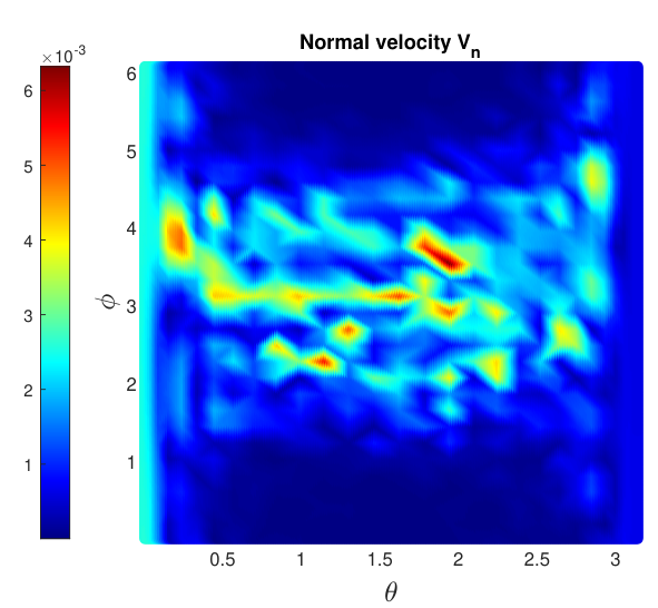
Fig. 6 shows the normal velocity $v_{n}$ on the source $\partial D_{a}$ in the rectangular $(\theta,\phi)$-plot. The pointwise amplitudes of $v_{n}$ are quite small and within order $10^{-2}$. The average power and stored energy in the actual source are 8.2197 dB and 9.1525 dB, respectively, which implies that it is feasible for physical implementation.

In this subsection we show the performance of our scheme in creating null fields in $D_{1}$ and $D_{2}$ while approximating two distinct prescribed patterns $f_{\infty,1},f_{\infty,2}$ in far-field directions ${\bf x}_{1}$ and ${\bf x}_{2}$, respectively (see Fig. 3(b) for one possible configuration). One possible application of this configuration would be a strategy to establish and maintain communication in several given far-field directions while avoiding near field interference located in $D_{1}$ and $D_{2}$. In this test, $k=10$, $D_{1}\Subset W_{1}$ with $W_{1}$ defined in (29) while $D_{2}\Subset W_{2}$ with $W_{2}$ given in the spherical coordinates as

$$\begin{split}W_{2}=&\left\{(r,\theta,\phi):r\in[1.0,1.2],\theta\in\left[\frac{\pi}{4},\frac{3\pi}{4}\right],\right.\left.\phi\in\left[-\frac{\pi}{4},\frac{\pi}{4}\right]\right\}.\end{split}$$

(31)

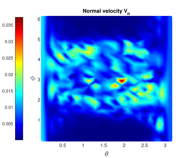
In this geometry, ${\bf x}_{1}=(r,\theta,\phi)=(r,\frac{\pi}{2},\pi)$ and ${\bf x}_{2}=(r,\theta,\phi)=(r,\frac{\pi}{2},0)$, $r\gg 1$ while the prescribed far-field pattern values are, $f_{\infty,1}=0.01+i\cdot 0.02$ in direction ${\bf x}_{1}$ and $f_{\infty,2}=0.05+i\cdot 0.03$ in direction ${\bf x}_{2}$. The simulation results are shown in Fig. 7, Fig. 8 and Fig. 9. In Fig. 7, we see that the absolute errors in the two near controls are within order $10^{-7}$. In Fig. 8 we present the good performance in two small patches of the far field centered in each of the two prescribed far field directions. In fact, when measured exactly in ${\bf x}_{1}$ and ${\bf x}_{2}$, the relative errors of the real parts are $3.2925\times 10^{-7}$ and $6.3876\times 10^{-8}$ while the relative errors of the imaginary part are $8.0229\times 10^{-8}$ and $1.6111\times 10^{-7}$, respectively. In Fig. 9 we present the normal velocity required on the actual physical source $D_{a}$. The average radiated power is 8.3986 dB and the stored energy is 9.6504 dB. The power budget is slightly larger than that in Section 3.1 as the source is projecting two non-zero far-field patterns in two directions.

The aforementioned results support the analysis of  [50] and show that our strategy produces good results for each of the two configurations depicted in Fig. 3. In the following tests, we aim to study the sensitivity of our strategy with respect to variations in several physically relevant parameters, such as wavenumber $k$, the distance between the control region and the active source, the control region size and, mutual distance between the control regions (in the case of more control regions and far field directions Fig. 3(b)). The feasibility of the active control scheme is also discussed by looking at the overall control accuracy, power budget, and anti-noise performance. The geometry in the sensitivity analysis is depicted in Fig. 10. To distinguish the original region (dark), the regions with modified parameters are shown in a light color. For instance, $D^{*2}_{1}$ denotes the near control which is shifted away from the active source, in which the superscript ‘2’ is corresponds to the experiment number in Section 3.3.2.

We start from the initial geometry in Fig. 3(a) but with $k=1$ and recall, in the spirit of [50], the performance of our strategy. In $D_{1}$ we prescribe a null field, and the desired far-field pattern value is $f_{\infty,1}=0.01+i\cdot 0.02$. The results are shown in Fig. 15, Fig. 16 and Fig. 17. From Fig. 15 we can observe that the maximum magnitude of the generated field in $D_{1}$ is within order $10^{-5}$. Similarly, Fig. 16 shows the pointwise relative error in the real and imaginary parts of the far field pattern. In the exact direction ${\bf x}_{1}$, the relative errors of the real part and imaginary part are $5.2449\times 10^{-4}$ and $1.8277\times 10^{-4}$, respectively. In Fig. 17, we show the boundary input $v_{n}$ on the actual source $\partial D_{a}$. Consequently, the average power and stored energy on the actual source are 11.2158 dB and 11.5906 dB, respectively. The power budget at this level allows the physical source implementation.

In this subsection we repeat the same experiments performed in the free space environment to explore the limitations or challenges of the active control in the homogeneous ocean environment. We only present here the effect of frequency and of the mutual distance between the near control and the source on the control accuracy and power budget. Some other experiment results are available in the supplementary material [55].

References

- [1] U. Gabbert, S. Ringwelski, Active vibration and noise control of a car engine: modeling and experimental validation, in: Mechanics and Model-Based Control of Advanced Engineering Systems, Springer, 2014, pp. 123–135.
- [2] S. Wang, H. Sun, J. Pan, X. Qiu, Near-field error sensing for active directivity control of radiated sound, The Journal of the Acoustical Society of America 144 (2) (2018) 598–607.
- [3] N. V. George, G. Panda, Advances in active noise control: A survey, with emphasis on recent nonlinear techniques, Signal processing 93 (2) (2013) 363–377.
- [4] J. Pan, R. Paurobally, X. Qiu, Active noise control in workplaces, Acoustics Australia 44 (1) (2016) 45–50.
- [5] D. Sachau, S. Jukkert, N. Hövelmann, Development and experimental verification of a robust active noise control system for a diesel engine in submarines, Journal of Sound and Vibration 375 (2016) 1–18.
- [6] D. Eggler, H. Chung, F. Montiel, J. Pan, N. Kessissoglou, Active noise cloaking of 2d cylindrical shells, Wave Motion 87 (2019) 106–122.
- [7] J. Jiang, Y. Li, Review of active noise control techniques with emphasis on sound quality enhancement, Applied Acoustics 136 (2018) 139–148.
- [8] J.-W. Choi, Y.-H. Kim, Generation of an acoustically bright zone with an illuminated region using multiple sources, The Journal of the Acoustical Society of America 111 (4) (2002) 1695–1700.
- [9] S. J. Elliott, J. Cheer, H. Murfet, K. R. Holland, Minimally radiating sources for personal audio, The Journal of the Acoustical Society of America 128 (4) (2010) 1721–1728.
- [10] J. Cheer, S. J. Elliott, M. F. S. Gálvez, Design and implementation of a car cabin personal audio system, Journal of the Audio Engineering Society 61 (6) (2013) 412–424.
- [11] T. Betlehem, P. D. Teal, A constrained optimization approach for multi-zone surround sound, in: 2011 IEEE International Conference on Acoustics, Speech and Signal Processing (ICASSP), IEEE, 2011, pp. 437–440.
- [12] L.-J. Brännmark, A. Bahne, A. Ahlen, Compensation of loudspeaker–room responses in a robust mimo control framework, IEEE transactions on audio, speech, and language processing 21 (6) (2013) 1201–1216.
- [13] D. Eggler, M. Karimi, N. Kessissoglou, Active acoustic cloaking in a convected flow field, The Journal of the Acoustical Society of America 146 (1) (2019) 586–594.
- [14] F. G. Vasquez, G. W. Milton, D. Onofrei, Active exterior cloaking for the 2d laplace and helmholtz equations, Physical review letters 103 (7) (2009) 073901.
- [15] F. G. Vasquez, G. W. Milton, D. Onofrei, Exterior cloaking with active sources in two dimensional acoustics, Wave Motion 48 (2011) 515–524.
- [16] F. G. Vasquez, G. W. Milton, D. Onofrei, Broadband exterior cloaking, Optics Express 17 (17) (2009) 14800–14805.
- [17] D. A. B. Miller, On perfect cloaking, Optics Express 14 (25) (2006) 12457–12466.
- [18] S. J. Elliott, J. Cheer, Modeling local active sound control with remote sensors in spatially random pressure fields, The Journal of the acoustical Society of america 137 (4) (2015) 1936–1946.
- [19] W. Jung, S. J. Elliott, J. Cheer, Combining the remote microphone technique with head-tracking for local active sound control, The Journal of the Acoustical Society of America 142 (1) (2017) 298–307.
- [20] H. Chen, C. Chan, Acoustic cloaking in three dimensions using acoustic metamaterials, Applied physics letters 91 (18) (2007) 183518.
- [21] S. A. Cummer, J. Christensen, A. Alù, Controlling sound with acoustic metamaterials, Nature Reviews Materials 1 (3) (2016) 16001.
- [22] A. Greenleaf, Y. Kurylev, M. Lassas, G. Uhlmann, Invisibility and inverse problems, Bulletin of the American Mathematical Society 46 (1) (2009) 55–97.
- [23]
R. V. Kohn, J. Lu, B. Schweizer, M. I. Weinstein,
A variational perspective on cloaking
by anomalous localized resonance (2012).
URL https://arxiv.org/abs/1210.4823 - [24]
N. J. A. Egarguin, D. Onofrei, E. Platt,
Sensitivity analysis for
the active manipulation of helmholtz fields in 3d, Inverse Problems in
Science and Engineering 28 (3) (2020) 314–339.
URL https://doi.org/10.1080/17415977.2018.1555248 - [25]
N. J. A. Egarguin, S. Zeng, D. Onofrei, J. Chen,
Active control of
helmholtz fields in 3d using an array of sources, Wave Motion 94 (102523)
(2020) 1–27.
URL https://doi.org/10.1016/j.wavemoti.2020.102523 - [26] D. Onofrei, E. Platt, On the synthesis of acoustic sources with controllable near fields, Wave Motion 77 (2018) 12–27.
- [27] E. Friot, R. Guillermin, M. Winninger, Active control of scattered acoustic radiation: A real-time implementation for a three-dimensional object, Acta Acust. Acust. 92 (2006) 278–288.
- [28] S. Elliott, Signal Processing for Active Control, 1st Edition, Signal Processing and its Applications, Academic Press, 2000.
- [29] C. House, J. Cheer, S. Daley, On the use of virtual sensing for the real-time detection and active control of a scattered acoustic field, International Congress of Sound and Vibration (2019).
- [30] J. Cheer, Active control of scattered acoustic fields: cancellation, reproduction and cloaking, J. Acoust. Soc. Am. 140 (3) (2016) 1502–1512.
- [31] P. A. Nelson, S. J. Elliott, Active Control of Sound, Academic London, 1992.
- [32] D. Onofrei, Active manipulation of fields modeled by the helmholtz equation, Journal Of Integral Equations and Applications 26 (4) (2014) 553–579.
- [33] F. Jensen, W. Kuperman, M. Porter, H. Schmidt, Computational Ocean Acoustics, Springer, 2011.
- [34] J. L. Buchanan, R. P. Gilbert, A. Wirgin, Y. S. Xu, Marine Acoustics: Direct and Inverse Problems, SIAM, 2004.
- [35] J. B. Keller, J. S. Papadakis, Wave Propagation and Underwater Acoustics, no. 70 in Lecture Notes in Physics, Springer-Verlag, 1977.
- [36] S. M. Kuo, D. R. Morgan, Active noise control: a tutorial review, Proceedings of the IEEE 87 (6) (1999) 943–973.
- [37] T. Betlehem, W. Zhang, M. A. Poletti, T. D. Abhayapala, Personal sound zones: Delivering interface-free audio to multiple listeners, IEEE Signal Processing Magazine 32 (2) (2015) 81–91.
- [38] A. N. Norris, Acoustic cloaking, Acoust. Today 11 (1) (2015) 38–46.
- [39] M. Kadic, T. Bückmann, R. Schittny, M. Wegener, Metamaterials beyond electromagnetism, Reports on Progress in physics 76 (12) (2013) 126501.
- [40] E. Dong, Y. Zhang, Z. Song, T. Zhang, C. Cai, N. X. Fang, Physical modeling and validation of porpoises’ directional emission via hybrid metamaterials, National Science Review 6 (5) (2019) 921–928.
- [41] Y. Zhang, Z. Song, X. Wang, W. Cao, W. W. Au, Directional acoustic wave manipulation by a porpoise via multiphase forehead structure, Physical Review Applied 8 (6) (2017) 064002.
- [42] M. Poletti, T. Betlehem, Design of a prototype variable directivity loudspeaker for improved surround sound reproduction in rooms, in: Audio Engineering Society Conference: 52nd International Conference: Sound Field Control-Engineering and Perception, Audio Engineering Society, 2013.
- [43] B. Rafaely, D. Khaykin, Optimal model-based beamforming and independent steering for spherical loudspeaker arrays, IEEE transactions on audio, speech, and language processing 19 (7) (2011) 2234–2238.
- [44] C. M. Gussen, P. S. Diniz, M. L. Campos, W. A. Martins, F. M. Costa, J. N. Gois, A survey of underwater wireless communication technologies, J. Commun. Inf. Sys. 31 (1) (2016) 242–255.
- [45] M. Zora, G. Buscaino, C. Buscaino, F. D’Anca, S. Mazzola, Acoustic signals monitoring in shallow marine waters: Technological progress for scientific data acquisition, Procedia Earth and Planetary Science: The 2nd International Workshop on Research in Shallow Marine and Fresh Water Systems 4 (2011) 80 – 92.
- [46]
J. R. Buck, J. C. Preisig, M. Johnson, J. Catipovic,
Single-mode excitation in the
shallow-water acoustic channel using feedback control, IEEE Journal of
Oceanic Engineering 22 (2) (1997) 281–291.
URL https://doi.org/10.1109/48.585947 - [47] D. Peng, T. Gao, J. Zeng, Study on single-mode excitation in time-variant shallow water environment, Journal of Computational Acoustics 22 (01) (2014) 1440001.
- [48] N. C. Makris, P. Ratilal, A unified model for reverberation and submerged object scattering in a stratified ocean waveguide, The Journal of the Acoustical Society of America 109 (3) (2001) 909–941.
- [49] D. Onofrei, On the active manipulation of fields and applications. i - the quasistatic regime, Inverse problems 28 (10) (2012) 105009.
- [50]
N. J. A. Egarguin, D. Onofrei, C. Qi, J. Chen,
Active manipulation
of helmholtz scalar fields: Near field synthesis with directional far field
control, Inverse Problems (2020).
URL http://iopscience.iop.org/10.1088/1361-6420/aba106 - [51] J. Ahrens, The single-layer potential approach applied to sound field synthesis including cases of non-enclosing distributions of secondary sources (2010).
- [52] D. Colton, R. Kress, Integral equation methods in scattering theory, SIAM Series: Classics in Applied Mathematics, 72, 2013.
- [53] T. Bonesky, Morozov’s discrepancy principle and tikhonov-type functionals, Inverse Problems 25 (1) (2008) 015015.
- [54] D. Colton, R. Kress, Inverse Acoustic and Electromagnetic Scattering Theory, 3rd Edition, Springer-Verlag, 2013.
- [55]
C. Qi, N. J. A. Egarguin, D. Onofrei, J. Chen,
2020
jasa supplementary material (2020).
URL drive.google.com/file/d/12RDPHQHsdwuQDwFtc-NZvKw462x-5Dko/view?usp=sharing