1INTRODUCTION

Regularization Matters: A Nonparametric Perspective on Overparametrized Neural Network

Tianyang Hu* Wenjia Wang* Cong Lin Guang Cheng

hu478@purdue.edu Purdue University wenjiawang@ust.hk Hong Kong University of Science and Technology 52174404011@stu.ecnu.edu.cn East China Normal University chengg@purdue.edu Purdue University

Abstract

Overparametrized neural networks trained by gradient descent (GD) can provably overfit any training data. However, the generalization guarantee may not hold for noisy data. From a nonparametric perspective, this paper studies how well overparametrized neural networks can recover the true target function in the presence of random noises. We establish a lower bound on the $L_{2}$ estimation error with respect to the GD iterations, which is away from zero without a delicate scheme of early stopping. In turn, through a comprehensive analysis of $\ell_{2}$ -regularized GD trajectories, we prove that for overparametrized one-hidden-layer ReLU neural network with the $\ell_{2}$ regularization: (1) the output is close to that of the kernel ridge regression with the corresponding neural tangent kernel; (2) minimax optimal rate of the $L_{2}$ estimation error can be achieved. Numerical experiments confirm our theory and further demonstrate that the $\ell_{2}$ regularization approach improves the training robustness and works for a wider range of neural networks.

1 INTRODUCTION

Deep learning has shown outstanding empirical successes and demonstrates superior performance in many standard machine learning tasks, such as image classification [Krizhevsky et al. 2012, LeCun et al. 2015, He et al. 2016], generative modeling [Goodfellow et al. 2014, Arjovsky et al. 2017], etc. Despite common accusations of being a black box with no theoretical guarantee, deep neural network (DNN) tends to achieve higher accuracy than other classical methods in various prediction tasks, which attracts plenty of interests from researchers. In contrast to the huge empirical success, little is yet settled from the theoretical side why DNN outperforms other methods. Without enough understanding, practical use of deep learning models could be inefficient and unreliable.^†^† * These authors contributed equally to this work.

Recently, many efforts have been devoted to provable deep learning methods with algorithmic guarantees, particularly training overparametrized neural networks by gradient descent (GD) or other gradient-based optimization. It has been shown that with enough overparametrization, e.g., neural network width tends to infinity, training DNN resembles a kernel method with a specific kernel called as “neural tangent kernel” (NTK) [Jacot et al. 2018]. In the NTK regime, GD can provably minimize the training error to zero in both regression [Du et al. 2018, Li and Liang 2018, Arora et al. 2019, Zou and Gu 2019] and classification [Ji and Telgarsky 2019a, Ji and Telgarsky 2019b, Lyu and Li 2019] settings. Corresponding generalization error bounds are developed to ensure prediction performance on unseen data. However, a closer inspection of these generalization results reveals that they only hold under the noiseless assumption, i.e., the response variable is deterministic given the explanatory variables. For overparametrized neural networks, the training loss can be minimized to zero so that the generalization error equals the population loss, which cannot be zero in the presence of noises. As random noises are ubiquitous in the real world, theoretical guarantees and provable learning algorithms that take into account of random noises are much needed in practice.

In contrast, classic nonparametric statistics literature demonstrate that in the presence of noises, the $L_{2}$ estimation error can still go to zero with possibly optimal rates as established in Stone 1982. To further investigate how overparametrized neural networks trained via GD work and how well they can learn the underlying true function with noisy data, we consider the classic nonparametric regression setting. Suppose we observe data $\{(\bm{x}_{i},y_{i})\}_{i=1}^{n}$ , given by

\displaystyle y_{i}=f^{*}(\bm{x}_{i})+\epsilon_{i},

(1.1)

where $f^{*}$ is the ground truth, $\bm{x}_{i}\in\mathbb{R}^{d}$ , and $\epsilon_{i}$ ’s are i.i.d. random noises with mean 0 and finite variance $\sigma^{2}$ . In this work, we consider neural network estimators $\widehat{f}$ produced by overparametrized one-hidden-layer ReLU neural networks, where the number of neurons can be much larger than the sample size, and investigate how fast the $L_{2}$ estimation error $\left\lVert\widehat{f}-f^{*}\right\rVert_{2}$ converges to zero as sample size grows.

Note that the $L_{2}$ convergence rate critically depends on the assumptions of the true function, e.g., linearity, smoothness, boundedness, etc., based on which minimax lower bounds are established [Siegel 1957]. An estimation method is said to be minimax-optimal if its convergence rate achieves the lower bound, indicating that it performs the best in the worst possible scenario. The above nonparametric perspective provides a sharp characterization of the employed estimation method and complements the existing optimization/generalization framework.

The main contributions of this paper are:

•

We prove that overparametrized one-hidden-layer ReLU neural networks trained using GD do not recover the true function in the classic nonparametric regression setting (1.1), i.e., the $L_{2}$ estimation error is bounded away from zero as sample size goes to infinity. To predict well on unseen data, a delicate early stopping rule has to be deployed.
•

We analyze the $\ell_{2}$ -regularized GD trajectory and show that the $\ell_{2}$ penalty on network weights amounts to penalizing the reproducing kernel Hilbert space (induced by NTK) norm of the associated neural network. With $\ell_{2}$ regularization, overparametrized neural network trained by GD resembles the solution of kernel ridge regression.
•

We further prove that by adding proper $\ell_{2}$ regularization, overparametrized neural network trained by GD achieves the minimax-optimal $L_{2}$ convergence rate $n^{-{d}/{(4d-2)}}$ , in recovering the ground truth in (1.1).

The correspondence between overparametrized neural network trained by $\ell_{2}$ -regularized GD and kernel ridge regression is nontrivial and technically challenging. In spite of the well-established equivalence between NTK and infinite-width DNN trained by GD, there is a huge technical gap for finite-width overparametrized neural networks, especially when the training objective includes explicit regularization terms.

To sum up, this work broadens the current scope of the NTK literature and connects the recent advances in deep learning theory, e.g., analyzing the trajectory of GD updates, implicit bias of overparametrization, etc., to the classical results in nonparametric statistics. More specifically, our findings not only contribute to the theoretical (in particular, nonparametric) understanding of training overparametrized DNN on noisy data but also promotes the use of $\ell_{2}$ penalty or weight decay in practice for better theoretical guarantees.

2 RELATED WORKS

Neural Tangent Kernel

The seminal paper [Jacot et al. 2018] proves that the evolution of DNNs during training can be described by the so-called neural tangent kernel (NTK), which is central to characterize the convergence and generalization behaviors. Du et al. 2018, Arora et al. 2019, Li and Liang 2018 investigate specifically for one-hidden-layer ReLU neural networks and show explicitly that with enough overparametrization, the weight vectors and the corresponding NTK do not change much during GD training. Similar investigations have been done for other neural networks and other settings [Zou and Gu 2019, Ji and Telgarsky 2019b]. Among others, Arora et al. 2019, Cao and Gu 2019 provide generalization error bounds and provable learning scenarios, but only hold for noiseless data.

For noisy data, explicit regularizations have recently been considered in the NTK literature. Wei et al. 2019 promote the $\ell_{2}$ penalty when using NTK by showing that in a constructed classification example, sample efficiency can benefit from the regularization. Hu et al. 2020 consider classification with noisy labels and propose to add $\ell_{2}$ regularization to ensure robustness. However, their analyses only apply to the kernel estimator directly using NTK and only relate to infinite width neural networks, which greatly restricts the model class capacity. As pointed out before, bridging the technical gap between NTK and finite-width overparametrized neural networks is technically challenging when the training objective includes an $\ell_{2}$ regularization term and we should not take it for granted. Geifman et al. 2020 demonstrate the similarity between the Laplace kernels and ReLU NTKs. However, in order for NTK to be a good characterization of neural network training, how wide is wide enough remains an active field of research [Nitanda et al. 2019]. In comparison, we directly analyze GD trajectories of training finite-width neural networks (with and without $\ell_{2}$ regularization) and prove that the corresponding NTK solutions can be well-approximated after a polynomial number of GD iterations. To the best of our knowledge, we are among the first to rigorously establish the $L_{2}$ convergence rate for trained neural networks under noisy data. Nitanda and Suzuki 2020 recently provide similar convergence rate analysis by considering a particular penalized stochastic gradient descent algorithm but they require the neural network width to be exponential with $n$ .

Nonparametric Regression

In nonparametric statistics, Stone 1982 shows that when $f^{*}$ is $d$ -variate and $\beta$ -time differentiable, the optimal rate of convergence for the $L_{2}$ estimation error is $n^{-\beta/(2\beta+d)}$ . Many popular methods such as kernel methods, Gaussian process, splines, etc., achieve this rate. It has been recently shown that DNN (with certain structures) can also achieve optimal convergence rates [Yarotsky 2017, Schmidt-Hieber 2017, Bauer et al. 2019, Liu et al. 2019] and even for non-smooth functions [Imaizumi and Fukumizu 2018]. However, this type of results has two limitations. Firstly, they only apply to the empirical risk minimizer or some specially constructed DNNs without any algorithmic guarantee. Secondly, the theoretical analysis relies on delicate complexity control of the DNN family and cannot handle overparametrization, which is very common in practice. Therefore, the aforementioned results are less helpful in understanding deep neural network models with overparametrization and highly non-convex optimization properties.

Our algorithm-dependent statistical analysis bridges the gap between these two types of research. Based on the GD trajectories and the corresponding NTK, we are able to analyze the trained overparametrized neural networks within the nonparametric framework and show they can also achieve the optimal convergence rate with proper regularizations.

3 PRELIMINARIES

Notation

For any function $f(\bm{x}):\mathcal{X}\to\mathbb{R}$ , denote $\left\lVert f\right\rVert_{\infty}=\sup_{\bm{x}\in\mathcal{X}}|f(\bm{x})|$ and $\left\lVert f\right\rVert_{p}=(\int_{\mathcal{X}}|f(\bm{x})|^{p}d\bm{x})^{1/p}$ . For any vector $\bm{x}$ , $\left\lVert\bm{x}\right\rVert_{p}$ denotes its $p$ -norm, for $1\leq p\leq\infty$ . $L_{p}$ and $l_{p}$ are used to distinguish function norms and vector norms. For two given sequences $\{a_{n}\}_{n\in\mathbb{N}}$ and $\{b_{n}\}_{n\in\mathbb{N}}$ of real numbers, we write $a_{n}\lesssim b_{n}$ if there exists a constant $C>0$ such that $a_{n}\leq Cb_{n}$ for all sufficiently large $n$ . Let $\Omega(\cdot)$ be the counterpart of $O(\cdot)$ that $a_{n}=\Omega(b_{n})$ means $a_{n}\gtrsim b_{n}$ . Further, $a_{n}=\widetilde{O}(b_{n})$ and $a_{n}=\widetilde{\Omega}(b_{n})$ are used to indicate there are specific requirements for the multiplicative constants. We write $a_{n}\asymp b_{n}$ if $a_{n}\lesssim b_{n}$ and $a_{n}\gtrsim b_{n}$ . Let $[N]=\{1,\dots,N\}$ for $N\in\mathbb{N}$ and let $\lambda_{\min}(\bm{A})$ be the minimum eigenvalue of a symmetric matrix $\bm{A}$ . We use $\mathbb{I}$ to denote the indicator function and $\bm{I}_{d}$ to denote the $d\times d$ identity matrix. $N(\mathbf{\bm{\mu}},\bm{\Sigma})$ represents Gaussian distribution with mean ${\bm{\mu}}$ and covariance $\bm{\Sigma}$ and ${\rm poly}(t_{1},t_{2},\ldots)$ denotes some polynomial function with arguments $t_{1},t_{2},\ldots$ .

Neural Network Setup

Consider the one-hidden-layer ReLU neural network family $\mathcal{F}$ with $m$ nodes in the hidden layer, expressed as

f_{\bm{W},\bm{a}}(\bm{x})=\frac{1}{\sqrt{m}}\sum_{r=1}^{m}a_{r}\sigma(\bm{w}_{r}^{\top}\bm{x}),

where $\bm{x}\in\mathbb{R}^{d}$ denotes the input, $\bm{W}=(\bm{w}_{1},\cdots,\bm{w}_{m})\in\mathbb{R}^{d\times m}$ is the weight matrix in the hidden layer, $\bm{a}=(a_{1},\cdots,a_{m})^{\top}\in\mathbb{R}^{m}$ is the weight vector in the output layer, $\sigma(z)=\max\{0,z\}$ is the rectified linear unit (ReLU). The initial values of the weights are independently generated from

\displaystyle\bm{w}_{r}(0)~\sim~N({\bm{0}},\tau^{2}\bm{I}_{m}),~~a_{r}~\sim~\mathrm{unif}\{-1,1\},~~\forall r\in[m].

When $m\gg n$ , the neural network is highly overparametrized. As is usually assumed in the NTK literature [Arora et al. 2019, Hu et al. 2020, Bietti and Mairal 2019], we consider data on the unit sphere $\mathbb{S}^{d-1}$ , i.e., $\left\lVert\bm{x}_{i}\right\rVert_{2}=1$ for any $i\in[n]$ . Throughout this work, we further assume that $\bm{x}_{1},\ldots,\bm{x}_{n}$ are uniformly distributed on $\mathbb{S}^{d-1}$ so that $\mathbb{E}_{\bm{x}\sim{\rm unif}(\mathbb{S}^{d-1})}(\widehat{f}(\bm{x})-f^{*}(\bm{x}))^{2}$ and $\left\lVert f-f^{*}\right\rVert_{2}^{2}$ are equal up to a constant multiplier and thus will be used interchangeably.

Gradient Descent

Let $\bm{y}=(y_{1},\cdots,y_{n})^{\top}$ and $\bm{\epsilon}=(\epsilon_{1},\cdots,\epsilon_{n})^{\top}$ . Denote $u_{i}=f_{\bm{W},\bm{a}}(\bm{x}_{i})$ to be the network’s prediction on $\bm{x}_{i}$ and let $\bm{u}=(u_{1},...,u_{n})^{\top}$ . Without loss of generality, we consider fixing the second layer $\bm{a}$ after initialization and only training the first layer $\bm{W}$ by GD. Fixing the last layer is not a strong restriction since $a\cdot\sigma(z)=\mbox{sign}(a)\cdot\sigma(|a|z)$ and we can always reparametrize the network to have all $a_{i}$ ’s to be either $1$ or $-1$ . Denote the empirical squared loss as $\Phi(\bm{W})=\frac{1}{2}\left\lVert\bm{y}-\bm{u}\right\rVert_{2}^{2}.$ The gradient of $\Phi(\bm{W})$ w.r.t. $\bm{w}_{r}$ can be written as

\displaystyle\frac{\partial\Phi(\bm{W})}{\partial\bm{w}_{r}}=\frac{1}{\sqrt{m}}a_{r}\sum_{i=1}^{n}(u_{i}-y_{i})\mathbb{I}_{r,i}\bm{x}_{i},\quad r\in[m],

where $\mathbb{I}_{r,i}=\mathbb{I}\{\bm{w}_{r}^{\top}\bm{x}_{i}\geq 0\}$ . Then the GD update rule at the $k$ -th iteration is given by

\displaystyle\bm{w}_{r}(k+1)=\bm{w}_{r}(k)-\eta\frac{\partial\Phi(\bm{W})}{\partial\bm{w}_{r}}\biggm|_{\bm{W}=\bm{W}(k)},

where $\eta>0$ is the step size (a.k.a. learning rate). In the rest of this work, we use $k$ to index variables at the $k$ -th iteration, e.g., $u_{i}(k)=f_{\bm{W}(k),\bm{a}}(\bm{x}_{i})$ , etc. Define $\mathbb{I}_{r,i}(k)=\mathbb{I}\{\bm{w}_{r}(k)^{\top}\bm{x}_{i}\geq 0\}$ , $\bm{Z}(k)\in\mathbb{R}^{md\times n}$ that

\displaystyle\bm{Z}(k)=\frac{1}{\sqrt{m}}\begin{pmatrix}a_{1}\mathbb{I}_{1,1}(k)\bm{x}_{1}&\dots&a_{1}\mathbb{I}_{1,n}(k)\bm{x}_{n}\\ \vdots&\ddots&\vdots\\ a_{m}\mathbb{I}_{m,1}(k)\bm{x}_{1}&\dots&a_{m}\mathbb{I}_{m,n}(k)\bm{x}_{n}\end{pmatrix}

and $\bm{H}(k)=\bm{Z}(k)^{\top}\bm{Z}(k)$ . It is shown that matrices $\bm{Z}(k)$ and $\bm{H}(k)$ are close to $\bm{Z}(0)$ and $\bm{H}(0)$ , respectively for any $k$ , when $m$ is sufficiently large [Arora et al. 2019]. We can rewrite the GD update rule as

\displaystyle\mathrm{vec}(\bm{W}(k+1))=\mathrm{vec}(\bm{W}(k))-\eta\bm{Z}(k)(\bm{u}(k)-\bm{y}),

(3.1)

where $\mathrm{vec}(\bm{W})=(\bm{w}_{1}^{\top},\cdots,\bm{w}_{m}^{\top})^{\top}\in\mathbb{R}^{md\times 1}$ is the vectorized weight matrix.

Kernel Ridge Regression with NTK

The study of one-hidden-layer ReLU neural networks is closely related to the NTK defined as

	$\displaystyle h(\bm{s},\bm{t})=$	$\displaystyle\mathbb{E}_{\bm{w}\sim N(0,\bm{I}_{d})}\left(\bm{s}^{\top}\bm{t}\ \mathbb{I}\{\bm{w}^{\top}\bm{s}\geq 0,\bm{w}^{\top}\bm{t}\geq 0\}\right)$
	$\displaystyle=$	$\displaystyle\frac{\bm{s}^{\top}\bm{t}(\pi-\arccos(\bm{s}^{\top}\bm{t}))}{2\pi},$		(3.2)

where $\bm{s},\bm{t}$ are $d$ -dimensional vectors. It can be shown that $h$ is positive definite on the unit sphere $\mathbb{S}^{d-1}$ [Bietti and Mairal 2019]. Let the Mercer decomposition of $h$ be $h(\bm{s},\bm{t})=\sum_{j=0}^{\infty}\lambda_{j}\varphi_{j}(\bm{s})\varphi_{j}(\bm{t}),$ where $\lambda_{1}\geq\lambda_{2}\geq...\geq 0$ are the eigenvalues, and $\{\varphi_{j}\}_{j=1}^{\infty}$ is an orthonormal basis.

The following lemma states the decay rate of eigenvalues of the NTK associated with one-hidden-layer ReLU neural networks, as a key technical contribution of this work.

Lemma 3.1.

Let $\lambda_{j}$ be the eigenvalues of NTK $h$ defined above. Then we have $\lambda_{j}\asymp j^{-\frac{d}{d-1}}$ .

Let $\mathcal{N}$ denote the reproducing kernel Hilbert space (RKHS) generated by $h$ on $\mathbb{S}^{d-1}$ , equipped with norm $\left\lVert\cdot\right\rVert_{\mathcal{N}}$ . For an unknown function $f^{*}\in\mathcal{N}$ , the kernel ridge regression minimizes

\displaystyle\min_{f\in\mathcal{N}}\frac{1}{2}\sum_{i=1}^{n}(y_{i}-f(\bm{x}_{i}))^{2}+\frac{\mu}{2}\left\lVert f\right\rVert_{\mathcal{N}}^{2},

(3.3)

where $\mu>0$ is a tuning parameter controlling the regularization strength. The representer theorem says that the solution to (3.3) can be written as

\displaystyle\widehat{f}(\bm{x})=h(\bm{x},\bm{X})(\bm{H}^{\infty}+\mu\bm{I}_{n})^{-1}\bm{y}

(3.4)

for any point $\bm{x}\in\mathbb{R}^{d}$ , where $h(\bm{x},\bm{X})=(h(\bm{x},\bm{x}_{1}),...,h(\bm{x},\bm{x}_{n}))\in\mathbb{R}^{1\times n}$ and $\bm{H}^{\infty}=\left(h(\bm{x}_{i},\bm{x}_{j})\right)_{n\times n}$ ( $\bm{H}^{\infty}$ is usually called the NTK matrix). In the following theorem, we show that the function $\widehat{f}$ is close to the true function $f^{*}$ under the $L_{2}$ metric.

Theorem 3.2.

Let $\widehat{f}$ be as in (3.4). By choosing $\mu\asymp n^{(d-1)/(2d-1)}$ , we have

\displaystyle\left\lVert\widehat{f}-f^{*}\right\rVert_{2}^{2}=O_{\mathbb{P}}\left(n^{-\frac{d}{2d-1}}\right),\quad\left\lVert\widehat{f}\right\rVert_{\mathcal{N}}^{2}=O_{\mathbb{P}}(1).

The proof of the convergence rate requires an accurate characterization of the complexity of $\mathcal{N}$ , which is determined by the eigenvalues and eigenfunction expansion of the NTK $h$ . If the eigenvalues decay at rate $\lambda_{j}\asymp j^{-2\nu}$ , the corresponding minimax optimal rate is $n^{-2\nu/(2\nu+1)}$ [Yuan et al. 2016, Raskutti et al. 2014]. Building on the the eigenvalue decay rate established in Lemma 3.1, it can be shown that the $L_{2}$ estimation rate in Theorem 3.2 is minimax-optimal.

In the rest of this work, we assume that $f^{*}\in\mathcal{N}$ .

4 PROBLEMS OF GRADIENT DESCENT FROM THE NONPARAMETRIC PERSPECTIVE

In this section, we consider training overparametrized neural networks with the GD update rule (3.1). Among others, Arora et al. 2019, Du et al. 2018 prove that as iteration $k\to\infty$ , the training data are interpolated, achieving zero training loss. However, in the presence of noises, i.e., $\epsilon_{i}$ in (1.1), such an overfitting to the training data can be harmful for recovering the ground truth. The following theorem shows that if $k$ is too small or too large, the $L_{2}$ estimation error of the trained neural network is bounded away from zero.

Theorem 4.1.

Fix a failure probability $\delta\in(0,1)$ . Let $\lambda_{0}$ be the largest number that with probability at least $1-\delta$ , $\lambda_{\min}(\bm{H}^{\infty})\geq\lambda_{0}$ . Suppose $m\geq\tau^{-2}{\rm poly}\left(n,\frac{1}{\lambda_{0}},\frac{1}{\delta}\right)$ , $\eta=\widetilde{O}\left(\frac{\lambda_{0}}{n^{2}}\right)$ , and $\tau=\widetilde{O}\left(\frac{\lambda_{0}\delta}{n}\right)$ . For sufficiently large $n$ , if the iteration $k=\widetilde{\Omega}\left(\frac{\log n}{\eta\lambda_{0}}\right)$ or $k=\widetilde{O}\left(\frac{1}{n\eta}\right)$ , then with probability at least $1-2\delta$ , we have

\mathbb{E}_{\bm{\epsilon}}\left\lVert f_{\bm{W}(k),\bm{a}}-f^{*}\right\rVert_{2}^{2}=\Omega(1).

The conditions on $m,\eta,$ and $\tau$ have the same rates as those in Theorem 5.1 of Arora et al. 2019, but the constants requirements are different. The probability $1-2\delta$ in Theorem 4.1 comes from the randomness of $\lambda_{\min}(\bm{H}^{\infty})$ and $(\bm{W}(0),\bm{a})$ .

Theorem 4.1 states that the estimation error for non-regularized one-hidden-layer neural networks is bounded away from zero by some constant if trained for too short or too long. The latter scenario indicates that overfitting is harmful in terms of the $L_{2}$ estimation error. Similar results have been shown in Kohler and Krzyzak 2019 for specifically designed overparametrized DNNs that is a linear combination of $\Omega(n^{10d^{2}})$ smaller neural networks, which is much more restrictive than ours.

In order to have low $L_{2}$ estimation errors, Theorem 4.1 implies that the iteration number $k$ must satisfy $(\eta\lambda_{0})^{-1}\log n\lesssim k\lesssim(n\eta)^{-1}$ . However, deriving a precise order of $k$ , which leads to the optimal rate of convergence, could be extremely challenging. Alternatively, we consider the infinite-width limit of one-hidden-layer ReLU networks, i.e., directly using the NTK (3) in kernel regression. This may shed some light on the optimal stopping time for practical overparametrized neural networks.

In kernel regression, the objective becomes

\displaystyle\min_{f\in\mathcal{N}}\frac{1}{2}\sum_{i=1}^{n}(y_{i}-f(\bm{x}_{i}))^{2},

(4.1)

whose solution can be explicitly expressed as $h(\bm{x},\bm{X})(\bm{H}^{\infty})^{-1}\bm{y}$ , by setting $\mu=0$ in (3.4). However, inverting the kernel matrix can be computationally intensive. In practice, gradient-based methods are often applied to solve (4.1) [Raskutti et al. 2014]. The following theorem establishes estimation error results for the NTK estimators trained by GD, complementary to Theorem 4.1.

Theorem 4.2.

Consider using GD to optimize (4.1) with a sufficiently small step size $\eta$ depending on $n$ (but not on $k$ ). There exists a stopping time $k^{*}$ depending on data, such that

\mathbb{E}\left\lVert\widehat{f}_{k^{*}}-f^{*}\right\rVert_{2}^{2}=O\left(n^{-\frac{d}{2d-1}}\right),

where $\widehat{f}_{k}$ is the predictor obtained at the $k$ -th iteration. Moreover, if $k\to\infty$ , the interpolated estimator $\widehat{f}_{\infty}$ satisfies

\mathbb{E}\left\lVert\widehat{f}_{\infty}-f^{*}\right\rVert_{2}^{2}=\Omega(1).

To specify the optimal stopping time $k^{*}$ in Theorem 4.2, we first introduce the local empirical Rademacher complexity defined as

\widehat{\mathcal{R}}_{\bm{H}^{\infty}}(\varepsilon):=\left(\frac{1}{n}\sum_{i=1}^{n}\min\big\{{\widehat{\lambda}_{i}}/{n},\varepsilon^{2}\big\}\right)^{1/2},

which relies on the eigenvalues $\widehat{\lambda}_{1}\geq\cdots\geq\widehat{\lambda}_{n}>0$ of $\bm{H}^{\infty}$ . Then, the stopping time $k^{*}$ is defined to be

\displaystyle k^{*}

\displaystyle:=\mathop{\mathrm{argmin}}\biggr\{k\in\mathbb{N}\,\mid\widehat{\mathcal{R}}_{\bm{H}^{\infty}}\big(\frac{1}{\sqrt{\eta{k}}}\big)>\frac{1}{2e\sigma\eta{k}}\biggr\}-1.

(4.2)

In essence, the optimal stopping time decreases with the noise level $\sigma$ and increases with the model complexity, measured by the eigenvalues of $\bm{H}^{\infty}$ .

Remark 1.

( $k^{*}$ for neural networks) To derive the order of $k^{*}$ for overparametrized neural network, a sharp characterization of the eigen-distribution of $\bm{H}^{\infty}$ is needed. To the best of the authors’ knowledge, no such results are available yet. Even though as $m\to\infty$ , neural network resembles its linearization (NTK), it doesn’t necessarily mean such a stopping rule can be easily derived for finite-width neural networks. In general, theoretical guarantees of an early stopping rule for training overparametrized neural networks is challenging and left for future work.

Besides early stopping, explicit regularizations are usually employed in deep learning models to balance the bias-variance trade-off and prevent overfitting, for example, weight decay [Krogh and Hertz 1992], batch normalization [Ioffe and Szegedy 2015], dropout [Srivastava et al. 2014], etc., to prevent overfitting. In the next section, we investigate the $\ell_{2}$ regularization [Bilgic et al. 2014, Van Laarhoven 2017, Phaisangittisagul 2016] and demonstrate its effectiveness in the nonparametric regression setting.

5 $\ell_{2}$ -REGULARIZED GRADIENT DESCENT FOR NOISY DATA

Without any regularization, GD overfits the training data and the estimation error is bounded away from zero. Instead, we propose using the $\ell_{2}$ -regularized gradient descent defined as

	$\displaystyle{\rm vec}(\bm{W}_{D}(k+1))=$	$\displaystyle{\rm vec}(\bm{W}_{D}(k))-\eta_{1}\bm{Z}_{D}(k)(\bm{u}_{D}(k)-\bm{y})$
		$\displaystyle-\eta_{2}\mu{\rm vec}(\bm{W}_{D}(k)),$		(5.1)

where $\eta_{1},\eta_{2}>0$ are step sizes, and $\mu>0$ is a tuning parameter. It can be easily seen that (5) is the GD update rule on the following loss function

\displaystyle\Phi_{1}(\bm{W})=\frac{1}{2}\left\lVert\bm{y}-\bm{u}\right\rVert_{2}^{2}+\frac{\mu}{2}\left\lVert{\rm vec}(\bm{W})\right\rVert_{2}^{2}.

(5.2)

The $\ell_{2}$ regularization has long been used in practical training neural networks and is equivalent to “weight decay” [Krogh and Hertz 1992] when using GD [Loshchilov and Hutter 2017]. In the NTK literature, $\ell_{2}$ regularization is also considered as a way to improve generalization [Wei et al. 2019, Hu et al. 2020]. However, we are among the first to directly analyze the $\ell_{2}$ -regularized GD trajectories of overparametrized neural networks and show its connection to kernel ridge regression using NTK. In the rest of this work, we use subscript $D$ to denote the variables under the regularized GD (5), e.g., $\bm{u}_{D}(k)$ for the predictions at the $k$ -th iteration.

Theorem 5.1.

Let $\lambda_{0}$ be the largest number such that with probability at least $1-\delta_{n}$ , $\lambda_{\min}(\bm{H}^{\infty})\geq\lambda_{0}$ , and $\delta_{n}\rightarrow 0$ as $n$ goes to infinity¹¹ 1 Potential dependency of $\lambda_{0}$ on $n$ is suppressed for notational simplicity.. For sufficiently large $n$ , suppose $\mu\asymp n^{\frac{d-1}{2d-1}}$ , $\eta_{1}\asymp\eta_{2}=o(n^{-\frac{3d-1}{2d-1}})$ , $\tau=O(1)$ , $m\geq\tau^{-2}{\rm ploy}(n,\lambda_{0}^{-1})$ , and the iteration number $k$ satisfies $\log\left({\rm ploy}_{1}(n,\tau,1/\lambda_{0})\right)\lesssim\eta_{2}\mu k\lesssim\log\left({\rm ploy}_{2}(\tau,1/n,\sqrt{m})\right).$ Then we have

	$\displaystyle\left\lVert\bm{u}_{D}(k)-\bm{H}^{\infty}(C\mu I+\bm{H}^{\infty})^{-1}\bm{y}\right\rVert_{2}=O_{\mathbb{P}}\left(\sqrt{n}(1-\eta_{2}\mu)^{k}\right),$		(5.3)
	$\displaystyle\left\lVert{\rm vec}(\bm{W}_{D}(k))-(1-\eta_{2}\mu)^{k}{\rm vec}(\bm{W}_{D}(0))\right\rVert_{2}=O_{\mathbb{P}}(1),$		(5.4)

for some constant $C>0$ . Moreover, during the training process, the mean squared loss satisfies

\displaystyle\Phi(\bm{W}_{D}(k))/n\leq(1-\eta_{2}\mu)^{k}\Phi(\bm{W}_{D}(0))/n+O_{\mathbb{P}}(1).

(5.5)

In the above theorem, three upper bounds are provided. In (5.3), we provide an upper bound on the difference between the prediction using one-hidden-layer neural networks and that obtained by (3.4), which converges to zero as the sample size goes to infinity. This indicates that the $\ell_{2}$ penalty on neural network weights has similar effects to penalizing the RKHS norm as in (3.3). Combining (5.3) and Theorem 3.2, we can conclude that the $\ell_{2}$ -regularized one-hidden-layer ReLU neural network recovers the true function on the training data points $\bm{x}_{1},\ldots,\bm{x}_{n}$ .

In (5.4), we provide an upper bound on the distance between the weight matrix at the $k$ -th iteration and the “decayed” initialization $\bm{W}_{D}(0)$ . Under the conditions in Theorem 5.1, their distance measured in Frobenius norm is bounded by some constant depending on the underlying true function. Unlike the results in Arora et al. 2019, the upper bound presented in (5.4) does not depend on data. Therefore, as long as the underlying function is within the RKHS generated by NTK, the total movement of all the weights is not large even if the data observed are corrupted by noises.

In (5.5), we give a characterization of how the training objective decreases over iterations, which is reminiscent of Theorem 4.1 in Du et al. 2018. Unlike the results without regularization, our $\ell_{2}$ -regularized objective is not expected to converge to zero, i.e., no data interpolation, which is essential to ensure the best trade-off between the bias and variance.

Remark 2.

(More iterations) The required iteration number $k$ in Theorem 5.1 is approximately $(\eta_{2}\mu)^{-1}$ , up to a logarithmic term. We believe the upper bound on $k$ is not necessary and may be relaxed. The stated results are expected to hold if $k\to\infty$ and we conjecture that the output will converge to the optimal solution of kernel ridge regression as in (3.4). Simulation results in Section 6 support our conjecture and we leave the technical proof for future work.

Next, we extend the results in Theorem 5.1 and establish the $L_{2}$ convergence rate for neural networks trained with $\ell_{2}$ -regularized GD.

Theorem 5.2.

Suppose the assumptions of Theorem 5.1 hold. Then we have

\left\lVert f_{\bm{W}_{D}(k),\bm{a}}-f^{*}\right\rVert_{2}^{2}=O_{\mathbb{P}}(n^{-\frac{d}{2d-1}}).

The above theorem states that with probability tending to one, the neural network estimator can still recover the true function with the optimal convergence rate of $n^{-\frac{d}{2(2d-1)}}$ , demonstrating the effectiveness of the $\ell_{2}$ regularization for noisy data. Unlike other optimality results established for neural networks [Schmidt-Hieber 2017, Bauer et al. 2019], our convergence rate result applies to overparametrized networks and is obtainable using the $\ell_{2}$ -regularized GD.

6 NUMERICAL STUDIES

In practice, regularization techniques are widely used in training deep learning models. Among others, Van Laarhoven 2017, Caruana et al. 2001, Prechelt 1998, Zhang et al. 2016, Lewkowycz and Gur-Ari 2020 have investigated the effectiveness of $\ell_{2}$ regularization and early stopping in training DNNs, and comprehensive comparisons have been made empirically against other regularization techniques. Therefore, one major goal of this section is not to show state-of-the-art performance using $\ell_{2}$ regularization, but to use it as an example to illustrate, from a nonparametric perspective, the necessity of regularization in training overparametrized neural networks with GD. Another goal is to demonstrate the robustness of our theory when some underlying assumptions are violated, e.g., one hidden layer, ReLU activation function and data on a sphere, etc.

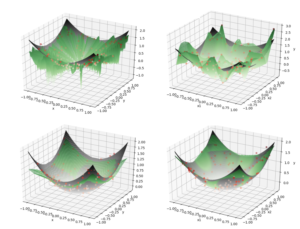
(a)

f^{*}_{1}

(b)

f^{*}_{2}

Figure 1: The

L_{2}

estimation errors are shown for all methods vs.

\sigma

, with their standard deviations plotted as vertical bars. Similarly for both

f^{*}_{1}

and

f^{*}_{2}

, we observe that NTK and ONN do not recover the true function well. Early stopping and

\ell_{2}

regularization perform similarly for NTK, especially for

f^{*}_{2}

. ONN

+\ell_{2}

performs the best in both cases.

Specifically, we consider NTK without regularization (NTK), NTK with early stopping²² 2 As specified in Theorem 4.2, the optimal stopping time $k^{*}$ in (4.2) depends on $\sigma$ , which is to be estimated from data. In our simulation, we directly use the true value. The GD algorithm can found in Appendix G (NTK+ES), NTK with $\ell_{2}$ regularization (NTK+ $\ell_{2}$ ), overparametrized neural network with and without $\ell_{2}$ regularization, denoted as ONN and ONN $+\ell_{2}$ , respectively. For ONN, we use two-hidden-layer ReLU neural networks and $m=500$ for each layer. To train the neural networks, instead of GD, we consider the more popular RMSProp optimizer [Hinton et al.] with the default setting. For ONN $+\ell_{2}$ and NTK $+\ell_{2}$ , the tuning parameter $\mu$ is selected by cross-validation.

6.1 Simulated Data

Consider the $d=2$ case where the training data points $\bm{x}_{1},\ldots,\bm{x}_{n}$ are i.i.d. sampled from unif $([-1,1]^{2})$ . We set $n=100$ and let noises follow $N(0,\sigma^{2})$ . Two target functions are considered: $f^{*}_{1}(\bm{x})=0$ and $f^{*}_{2}(\bm{x})=\bm{x}^{\top}\bm{x}$ . The $L_{2}$ estimation error is approximated using a noiseless test dataset $\{(\bar{\bm{x}}_{i},f^{*}(\bar{\bm{x}}_{i}))\}_{i=1}^{1000}$ where $\bar{\bm{x}}_{i}$ ’s are new samples i.i.d. from unif $([-1,1]^{2})$ . We choose $\sigma=0.1,0.2,...,0.5$ and for each $\sigma$ value, $100$ replications are run to estimate the mean and standard deviation of the $L_{2}$ estimation error. Results are presented in Figure 1. More details and results can be found in Appendix G.

6.2 Real Data

To showcase our results on the $L_{2}$ estimation, an ideal dataset is one that can be well-fitted by neural networks so that we can treat it as noiseless and then manually inject random noises. Inspired by the numerical studies in Hu et al. 2020, we consider the MNIST dataset (digits 5 vs. 8 relabeled as $-1$ and $1$ ), where the test accuracy can reach over 99% by shallow fully connected neural networks [LeCun et al. 1998]. Even though the dataset is for classification, we can treat the labels as continuous and learn the true function under the proposed regression setting. We use $\bm{y}^{*}$ to denote the true labels and manually add noises $\bm{\epsilon}$ to the training data, where each element of $\bm{\epsilon}$ follows $N(0,\sigma^{2})$ independently. The perturbed labels are denoted by $\bm{y}=\bm{y}^{*}+\bm{\epsilon}$ . By gradually increase $\sigma$ , we investigate how ONN and ONN $+\ell_{2}$ perform under the additive label noises setting.

Remark 3.

(Additive label noises) To manually inject noises to classification data, many works consider replacing part of the labels by random labels [Zhang et al. 2016, Arora et al. 2019]. However, such noises are not i.i.d. and cannot be applied to the regression setting. Similar additive label noises are also considered in Hu et al. 2020.

The training dataset contains $n=11272$ vectorized images of dimension $d=784$ . The test dataset size is 1866. For ONN $+\ell_{2}$ , our training objective function is $\Phi_{1}$ as in (5.2) and setting $\mu=0$ corresponds to the objective function of training ONN. On test dataset, which is not contaminated by noises, we use the sign of the output for classification and calculate the misclassification rate as a measure of estimation performance. To be more specific, a test image $\bar{\bm{x}}$ is classified as label 8 if $\widehat{f}(\bar{\bm{x}})\geq 0$ , and label 5 if $\widehat{f}(\bar{\bm{x}})<0$ , where $\widehat{f}$ is the neural network estimator. The misclassification rate is the percentage of incorrect classifications on the test images. We choose $\sigma=0,0.25,...,1.5$ and for each $\sigma$ value, $100$ replications are run to estimate the mean and standard deviation of the test misclassification rate. How the training root mean square error (RMSE) and test misclassification rate evolve during training when $\sigma=1$ for ONN and ONN $+\ell_{2}$ is also investigated. The results are reported in Figure 2. More details and results can be found in Appendix G.

Figure 2: Figure (a) shows the test misclassification rates for all methods vs.

\sigma

with their standard deviations plotted as vertical bars. NTK+ES for

\sigma=0

is omitted since

k^{*}

is not well-defined when

\sigma=0

and NTK+ES in this case should be the same as NTK, i.e.

k^{*}=\infty

. As

\sigma

increases, all misclassification rates increase but NTK

+\ell_{2}

and ONN

+\ell_{2}

perform significantly better than NTK and ONN with smaller misclassification rate and better stability, i.e., the standard deviation is smaller. The NTK+ES is the green line and it performs the worst when

\sigma\leq 0.5

but better than NTK and ONN when

\sigma\geq 1

. Figure (b) shows how the training RMSE and test misclassification rate evolve across iterations for ONN and ONN

+\ell_{2}

when

\sigma=1

. For both methods, the training RMSEs decrease fast in the first 1K iterations. However, as the ONN training RMSE flattens after 10K iterations, its test misclassification rate goes up while that for ONN

+\ell_{2}

remains flat even after 50K iterations, which supports our conjecture in Remark 2. Figure (b) also reveals the potential early stopping time for ONN around iteration 10K, which has test misclassification rate comparable to that of ONN

+\ell_{2}

Remark 4.

(NTK+ES) The performance of NTK+ES is shown in Figure 2. Unlike in the simulated dataset where NTK+ES and NTK $+\ell_{2}$ perform almost identically, NTK+ES performs noticeably worst for the MNIST dataset, especially when $\sigma$ is small. One possible explanation lies in our additive label noise setting. Even though we treat the labels as continuous during training, the reported misclassification rate only depends on the sign of the label. If $\sigma$ is small, the probability of changing signs is small. This may be one of the reasons that NTK, ONN perform relatively well for small $\sigma$ ’s, since if the signs remain the same, it is not very harmful to overfit the labels. Note that NTK+ $\ell_{2}$ and ONN+ $\ell_{2}$ choose small $\mu$ ’s such that it is not very different from NTK and ONN. The stopping rule in NTK+ES, on the other hand, doesn’t take the classification setting into consideration and tends to underestimate the stopping time when the additive label noises are small. Nonetheless, we don’t recommend NTK+ES for handling large datasets. Firstly, the noise level $\sigma$ needs to be estimated, which brings extra instability to the algorithm. Secondly, NTK+ES is very computationally intensive, especially for the eigenvalues of the NTK matrix.

7 CONCLUSION AND DISCUSSION

From a nonparametric perspective, this paper studies overparametrized neural networks trained with GD and establishes optimal $L_{2}$ convergence rates for trained neural network estimators under the $\ell_{2}$ regularization. On one hand, our result broadens the NTK literature by incorporating an explicit penalty term in the training objective. On the other hand, our convergence analysis extends the statistical theory of deep neural networks by bringing algorithmic guarantees into the network estimator and offsetting the extra complexity from overparametrization through delicate GD analysis. Our simulation results corroborate the theoretical analysis and imply that the assumptions of our theory may be relaxed. More investigations along this direction would advance our statistical understandings of deep learning. For example, our work can be further improved by relaxing the sphere assumption on the input data and the iteration number $k$ imposed in Theorems 5.1 and 5.2. Additionally, although our theoretical analysis depends on the exact formula of the NTK associated with one-hidden layer ReLU neural network, it is possible to extend our theory to multi-layer DNNs as empirically shown in numerical experiments. In fact, it has been shown that the RKHS generated by the multi-layer NTK is equivalent to the one-hidden NTK [Chen and Xu 2020]. Therefore, one possible approach for generalizing our theory is based on this equivalence.

The nonparametric perspective is potentially helpful in understanding other popular regularization techniques, e.g., batch normalization [Ioffe and Szegedy 2015], data augmentation [Dao et al. 2019], knowledge distillation [Hinton et al. 2015], etc. On the other hand, novel and problem-specific regularization approaches may be motivated during the convergence analysis that inspires better performance in practice.

References

Krizhevsky et al. [2012] Alex Krizhevsky, Ilya Sutskever, and Geoffrey E Hinton. Imagenet classification with deep convolutional neural networks. In Advances in Neural Information Processing Systems, pages 1097–1105, 2012.
LeCun et al. [2015] Yann LeCun, Yoshua Bengio, and Geoffrey Hinton. Deep learning. Nature, 521(7553):436, 2015.
He et al. [2016] Kaiming He, Xiangyu Zhang, Shaoqing Ren, and Jian Sun. Deep residual learning for image recognition. In Proceedings of the IEEE Conference on Computer Vision and Pattern Recognition, pages 770–778, 2016.
Goodfellow et al. [2014] Ian Goodfellow, Jean Pouget-Abadie, Mehdi Mirza, Bing Xu, David Warde-Farley, Sherjil Ozair, Aaron Courville, and Yoshua Bengio. Generative adversarial nets. In Advances in Neural Information Processing Systems, pages 2672–2680, 2014.
Arjovsky et al. [2017] Martin Arjovsky, Soumith Chintala, and Léon Bottou. Wasserstein GAN. arXiv preprint arXiv:1701.07875, 2017.
Jacot et al. [2018] Arthur Jacot, Franck Gabriel, and Clément Hongler. Neural tangent kernel: Convergence and generalization in neural networks. In Advances in Neural Information Processing Systems, pages 8571–8580, 2018.
Du et al. [2018] Simon S Du, Xiyu Zhai, Barnabas Poczos, and Aarti Singh. Gradient descent provably optimizes over-parameterized neural networks. arXiv preprint arXiv:1810.02054, 2018.
Li and Liang [2018] Yuanzhi Li and Yingyu Liang. Learning overparameterized neural networks via stochastic gradient descent on structured data. In Advances in Neural Information Processing Systems, pages 8157–8166, 2018.
Arora et al. [2019] Sanjeev Arora, Simon S Du, Wei Hu, Zhiyuan Li, and Ruosong Wang. Fine-grained analysis of optimization and generalization for overparameterized two-layer neural networks. arXiv preprint arXiv:1901.08584, 2019.
Zou and Gu [2019] Difan Zou and Quanquan Gu. An improved analysis of training over-parameterized deep neural networks. In Advances in Neural Information Processing Systems, pages 2053–2062, 2019.
Ji and Telgarsky [2019a] Ziwei Ji and Matus Telgarsky. The implicit bias of gradient descent on nonseparable data. In Conference on Learning Theory, pages 1772–1798, 2019a.
Ji and Telgarsky [2019b] Ziwei Ji and Matus Telgarsky. Polylogarithmic width suffices for gradient descent to achieve arbitrarily small test error with shallow ReLU networks. arXiv preprint arXiv:1909.12292, 2019b.
Lyu and Li [2019] Kaifeng Lyu and Jian Li. Gradient descent maximizes the margin of homogeneous neural networks. arXiv preprint arXiv:1906.05890, 2019.
Stone [1982] Charles J Stone. Optimal global rates of convergence for nonparametric regression. The Annals of Statistics, pages 1040–1053, 1982.
Siegel [1957] Sidney Siegel. Nonparametric statistics. The American Statistician, 11(3):13–19, 1957.
Cao and Gu [2019] Yuan Cao and Quanquan Gu. Generalization error bounds of gradient descent for learning overparameterized deep ReLU networks. arXiv preprint arXiv:1902.01384, 2019.
Wei et al. [2019] Colin Wei, Jason D Lee, Qiang Liu, and Tengyu Ma. Regularization matters: Generalization and optimization of neural nets vs their induced kernel. In Advances in Neural Information Processing Systems, pages 9709–9721, 2019.
Hu et al. [2020] W Hu, Z Li, and D Yu. Simple and effective regularization methods for training on noisily labeled data with generalization guarantee. In International Conference on Learning Representations, 2020.
Geifman et al. [2020] Amnon Geifman, Abhay Yadav, Yoni Kasten, Meirav Galun, David Jacobs, and Ronen Basri. On the similarity between the laplace and neural tangent kernels. NeurIPS 2020, 2020.
Nitanda et al. [2019] Atsushi Nitanda, Geoffrey Chinot, and Taiji Suzuki. Gradient descent can learn less over-parameterized two-layer neural networks on classification problems. arXiv preprint arXiv:1905.09870, 2019.
Nitanda and Suzuki [2020] Atsushi Nitanda and Taiji Suzuki. Optimal rates for averaged stochastic gradient descent under neural tangent kernel regime. arXiv preprint arXiv:2006.12297, 2020.
Yarotsky [2017] Dmitry Yarotsky. Error bounds for approximations with deep ReLU networks. Neural Networks, 94:103–114, 2017.
Schmidt-Hieber [2017] Johannes Schmidt-Hieber. Nonparametric regression using deep neural networks with ReLU activation function. arXiv preprint arXiv:1708.06633, 2017.
Bauer et al. [2019] Benedikt Bauer, Michael Kohler, et al. On deep learning as a remedy for the curse of dimensionality in nonparametric regression. The Annals of Statistics, 47(4):2261–2285, 2019.
Liu et al. [2019] Ruiqi Liu, Ben Boukai, and Zuofeng Shang. Optimal nonparametric inference via deep neural network. arXiv preprint arXiv:1902.01687, 2019.
Imaizumi and Fukumizu [2018] Masaaki Imaizumi and Kenji Fukumizu. Deep neural networks learn non-smooth functions effectively. arXiv preprint arXiv:1802.04474, 2018.
Bietti and Mairal [2019] Alberto Bietti and Julien Mairal. On the inductive bias of neural tangent kernels. In Advances in Neural Information Processing Systems, pages 12873–12884, 2019.
Yuan et al. [2016] Ming Yuan, Ding-Xuan Zhou, et al. Minimax optimal rates of estimation in high dimensional additive models. The Annals of Statistics, 44(6):2564–2593, 2016.
Raskutti et al. [2014] Garvesh Raskutti, Martin J Wainwright, and Bin Yu. Early stopping and non-parametric regression: an optimal data-dependent stopping rule. The Journal of Machine Learning Research, 15(1):335–366, 2014.
Kohler and Krzyzak [2019] Michael Kohler and Adam Krzyzak. Over-parametrized deep neural networks do not generalize well. arXiv preprint arXiv:1912.03925, 2019.
Krogh and Hertz [1992] Anders Krogh and John A Hertz. A simple weight decay can improve generalization. In Advances in Neural Information Processing Systems, pages 950–957, 1992.
Ioffe and Szegedy [2015] Sergey Ioffe and Christian Szegedy. Batch normalization: Accelerating deep network training by reducing internal covariate shift. arXiv preprint arXiv:1502.03167, 2015.
Srivastava et al. [2014] Nitish Srivastava, Geoffrey Hinton, Alex Krizhevsky, Ilya Sutskever, and Ruslan Salakhutdinov. Dropout: a simple way to prevent neural networks from overfitting. The Journal of Machine Learning Research, 15(1):1929–1958, 2014.
Bilgic et al. [2014] Berkin Bilgic, Itthi Chatnuntawech, Audrey P Fan, Kawin Setsompop, Stephen F Cauley, Lawrence L Wald, and Elfar Adalsteinsson. Fast image reconstruction with l2-regularization. Journal of magnetic resonance imaging, 40(1):181–191, 2014.
Van Laarhoven [2017] Twan Van Laarhoven. L2 regularization versus batch and weight normalization. arXiv preprint arXiv:1706.05350, 2017.
Phaisangittisagul [2016] Ekachai Phaisangittisagul. An analysis of the regularization between l2 and dropout in single hidden layer neural network. In 2016 7th International Conference on Intelligent Systems, Modelling and Simulation (ISMS), pages 174–179. IEEE, 2016.
Loshchilov and Hutter [2017] Ilya Loshchilov and Frank Hutter. Decoupled weight decay regularization. arXiv preprint arXiv:1711.05101, 2017.
Caruana et al. [2001] Rich Caruana, Steve Lawrence, and C Lee Giles. Overfitting in neural nets: Backpropagation, conjugate gradient, and early stopping. In Advances in Neural Information Processing Systems, pages 402–408, 2001.
Prechelt [1998] Lutz Prechelt. Early stopping-but when? In Neural Networks: Tricks of the Trade, pages 55–69. Springer, 1998.
Zhang et al. [2016] Chiyuan Zhang, Samy Bengio, Moritz Hardt, Benjamin Recht, and Oriol Vinyals. Understanding deep learning requires rethinking generalization. arXiv preprint arXiv:1611.03530, 2016.
Lewkowycz and Gur-Ari [2020] Aitor Lewkowycz and Guy Gur-Ari. On the training dynamics of deep networks with $l\_2$ regularization. arXiv preprint arXiv:2006.08643, 2020.
[42] Geoffrey Hinton, Nitish Srivastava, and Kevin Swersky. Neural networks for machine learning lecture 6a overview of mini-batch gradient descent.
LeCun et al. [1998] Yann LeCun, Léon Bottou, Yoshua Bengio, and Patrick Haffner. Gradient-based learning applied to document recognition. Proceedings of the IEEE, 86(11):2278–2324, 1998.
Chen and Xu [2020] Lin Chen and Sheng Xu. Deep neural tangent kernel and laplace kernel have the same rkhs. arXiv preprint arXiv:2009.10683, 2020.
Dao et al. [2019] Tri Dao, Albert Gu, Alexander J Ratner, Virginia Smith, Christopher De Sa, and Christopher Ré. A kernel theory of modern data augmentation. Proceedings of machine learning research, 97:1528, 2019.
Hinton et al. [2015] Geoffrey Hinton, Oriol Vinyals, and Jeff Dean. Distilling the knowledge in a neural network. arXiv preprint arXiv:1503.02531, 2015.
Cao et al. [2019] Yuan Cao, Zhiying Fang, Yue Wu, Ding-Xuan Zhou, and Quanquan Gu. Towards understanding the spectral bias of deep learning. arXiv preprint arXiv:1912.01198, 2019.
van de Geer [2000] Sara van de Geer. Empirical Processes in M-estimation. Cambridge University Press, 2000.
van de Geer [2014] Sara van de Geer. On the uniform convergence of empirical norms and inner products, with application to causal inference. Electronic Journal of Statistics, 8(1):543–574, 2014.
Kimeldorf and Wahba [1971] George Kimeldorf and Grace Wahba. Some results on tchebycheffian spline functions. Journal of mathematical analysis and applications, 33(1):82–95, 1971.
Varga [2010] Richard S Varga. Gershgorin and His Circles, volume 36. Springer Science & Business Media, 2010.
Bach [2017] Francis Bach. Breaking the curse of dimensionality with convex neural networks. The Journal of Machine Learning Research, 18(1):629–681, 2017.
Atkinson and Han [2012] Kendall Atkinson and Weimin Han. Spherical Harmonics and Approximations on the Unit Sphere: An Introduction, volume 2044. Springer Science & Business Media, 2012.
Costas and Christopher [2014] Efthimiou Costas and Frye Christopher. Spherical Harmonics in $p$ Dimensions. World Scientific, 2014.
Brauchart and Dick [2013] Johann S Brauchart and Josef Dick. A characterization of Sobolev spaces on the sphere and an extension of Stolarsky’s invariance principle to arbitrary smoothness. Constructive Approximation, 38(3):397–445, 2013.
Wang et al. [2014] He Ping Wang, Kai Wang, and Jing Wang. Entropy numbers of Besov classes of generalized smoothness on the sphere. Acta Mathematica Sinica, English Series, 30(1):51–60, 2014.
Glorot and Bengio [2010] Xavier Glorot and Yoshua Bengio. Understanding the difficulty of training deep feedforward neural networks. In Proceedings of the thirteenth international conference on artificial intelligence and statistics, pages 249–256, 2010.

Supplementary Materials

Appendix A More notation

We introduce some additional notation to be used in the Appendix. Denote $\bm{y}^{*}=(f^{*}(x_{1}),\cdots,f^{*}(x_{n}))^{\top}$ as the the vector of underlying function’s functional values at sample points. Let $\mathbb{I}_{r}(\bm{x})=\mathbb{I}\{\bm{w}_{r}^{\top}\bm{x}\geq 0\}$ and

\displaystyle\bm{z}(\bm{x})=\frac{1}{\sqrt{m}}\begin{pmatrix}a_{1}\mathbb{I}_{1}(\bm{x})\bm{x}\\ \vdots\\ a_{m}\mathbb{I}_{m}(\bm{x})\bm{x}\end{pmatrix}\in\mathbb{R}^{md\times 1}.

(A.1)

Thus, $\bm{Z}(k)=(\bm{z}(\bm{x}_{1}),...,\bm{z}(\bm{x}_{n}))|_{\bm{W}=\bm{W}(k)}$ . When the context is clear, we omit the dimension and write $\bm{I}_{d}$ as $\bm{I}$ .

Appendix B Proof of Lemma 3.1

We will use the following lemma, which states the Mercer decomposition of $h$ as in (3).

Lemma B.1 (Mercer decomposition of NTK $h$ ).

For any $\bm{s},\bm{t}\in\mathbb{S}^{d-1}$ , we have the following decomposition of the NTK,

\displaystyle h(\bm{s},\bm{t})=\sum_{k=0}^{\infty}\mu_{k}\sum_{j=1}^{N(d,k)}Y_{k,j}(\bm{s})Y_{k,j}(\bm{t}),

where $Y_{k,j}$ , $j=1,...,N(d,k)$ are spherical harmonic polynomials of degree $k$ , and the non-negative eigenvalues $\mu_{k}$ satisfy $\mu_{k}\asymp k^{-d}$ , and $\mu_{k}=0$ if $k=2j+1$ for $k\geq 2$ .

The proof of Lemma B.1 is similar to the proof of Proposition 5 in Bietti and Mairal 2019. The difference is that the Proposition 5 in Bietti and Mairal 2019 considers the kernel function

\displaystyle h_{1}(\bm{s},\bm{t})=4h(\bm{s},\bm{t})+\frac{\sqrt{1-(\bm{s}^{\top}\bm{t})^{2}}}{\pi},

and we only need to consider the kernel function $h(\bm{s},\bm{t})$ . A generalization of Proposition 5 in Bietti and Mairal 2019 can be found in Theorem 3.5 of Cao et al. 2019.

Note that in the proof of Lemma B.1,

\displaystyle N(d,j)=\frac{2j+d-2}{j}\left(\begin{array}[]{c}j+d-3\\ d-2\end{array}\right)=\frac{\Gamma(j+d-2)}{\Gamma(d-1)\Gamma(j)},

where $\Gamma$ is the Gamma function. By the Stirling approximation, we have $\Gamma(x)\approx\sqrt{2\pi}x^{x-1/2}e^{-x}$ . Therefore, we have the number $N(d,j)$ is equivalent to $j^{d-2}$ . Thus, by Lemma B.1, the $j$ -th eigenvalue $\lambda_{j}$ can be denoted by

\displaystyle\lambda_{j}=\mu_{l},\mbox{ for }\sum_{i=1}^{l-1}N(d,2i)\leq j<\sum_{i=1}^{l}N(d,2i),

which can be approximated by $\lambda_{j}\asymp\mu_{l},\mbox{ for }(2l-2)^{d-1}\leq j<(2l)^{d-1}.$ By Lemma B.1, we have $\mu_{l}\asymp l^{-d}$ , which implies $\lambda_{j}\asymp j^{-\frac{d}{d-1}}$ .

Appendix C Proof of Theorem 3.2

Let $\mathcal{G}$ be a metric space equipped with a metric $d_{g}$ . The $\delta$ -covering number of the metric space $(\mathcal{G},d_{g})$ , denoted by $N(\delta,\mathcal{G},d_{g})$ , is the minimum integer $N$ so that there exist $N$ distinct balls in $(\mathcal{G},d_{g})$ with radius $\delta$ , and the union of these balls covers $\mathcal{G}$ . Let $H(\delta,\mathcal{G},d_{g})=\log N(\delta,\mathcal{G},d_{g})$ be the entropy of the metric space $(\mathcal{G},d_{g})$ . We first present an upper bound on the entropy of the metric space $(\mathcal{N},\left\lVert\cdot\right\rVert_{\infty})$ , where the proof can be found in Appendix F.

Lemma C.1.

Let $\mathcal{N}$ be the reproducing kernel Hilbert space generated by the NTK $h$ defined in (3), equipped with norm $\left\lVert\cdot\right\rVert_{\mathcal{N}}$ . The entropy $H(\delta,\mathcal{N}(1),\left\lVert\cdot\right\rVert_{\infty})$ can be bounded by

\displaystyle H(\delta,\mathcal{N}(1),\left\lVert\cdot\right\rVert_{\infty})\leq A_{0}\delta^{-\frac{2(d-1)}{d}},

(C.1)

where $\mathcal{N}(1)=\{f:f\in\mathcal{N},\left\lVert f\right\rVert_{\mathcal{N}}\leq 1\}$ , and $A_{0}>0$ is a constant not depending on $\delta$ .

For the regression problem, consider a general penalized least-square estimator

\widehat{f}:=\mathop{\mathrm{argmin}}_{f\in\mathcal{N}}\left(\frac{1}{n}\sum_{i=1}^{n}(y_{i}-f(\bm{x}_{i}))^{2}+\lambda_{n}^{2}I^{v}(f)\right),

where $\lambda_{n}>0$ is the smoothing parameter and $I:\mathcal{N}\to[0,\infty)$ is a pseudo-norm measuring the complexity. We use the RKHS norm $\left\lVert f\right\rVert_{\mathcal{N}}$ in our case. Let $\left\lVert\cdot\right\rVert_{n}$ denote the empirical norm. The following lemma establishes the rate of convergence for the estimator $\widehat{f}$ .

Lemma C.2 (Lemma 10.2 in van de Geer 2000).

Assume Gaussian noises and entropy bound $H(\delta,\mathcal{N}(1),\left\lVert\cdot\right\rVert_{n})\leq A\delta^{-\alpha}$ for some constants $A>0$ and $0<\alpha<2$ . If $v\geq\frac{2\alpha}{2+\alpha}$ , $I(f^{*})>0$ and

\lambda_{n}^{-1}=O_{\mathbb{P}}\left(n^{1/(2+\alpha)}\right)I^{(2v-2\alpha+v\alpha)/2(2+\alpha)}(f^{*}).

Then we have

\left\lVert\widehat{f}-f^{*}\right\rVert_{n}=O_{\mathbb{P}}(\lambda_{n})I^{v/2}(f^{*})

and $I(\widehat{f})=O_{\mathbb{P}}(1)I(f^{*})$ .

To bound the difference between empirical norm and $L_{2}$ norm, we utilize the following lemma. For a class of functions ${\cal F}$ , define for $z>0$

{J}_{\infty}(z,{\cal F}):=C_{0}\inf_{\delta>0}\biggl[z\int_{\delta/4}^{1}\sqrt{{\cal H}_{{\infty}}(uz/2,{\cal F})}du+\sqrt{n}\delta z\biggr].

Lemma C.3 (Theorem 2.2 in van de Geer 2014).

Let

R:=\sup_{f\in{\cal F}}\left\lVert f\right\rVert_{2},\ K:=\sup_{f\in{\cal F}}\left\lVert f\right\rVert_{\infty}

Then, for all $t>0$ , with probability at least $1-\exp[-t]$ ,

\sup_{f\in{\cal F}}\biggl|\left\lVert f\right\rVert_{n}^{2}-\left\lVert f\right\rVert_{2}^{2}\biggr|/C_{1}\leq\frac{2RJ_{\infty}(K,{\cal F})+RK\sqrt{t}}{\sqrt{n}}+\frac{4J_{\infty}^{2}(K,{\cal F})+K^{2}t}{n}

where $C_{1}>0$ is some constant not depending on $n$ .

Proof of Theorem 3.2.

Consider our estimator $\widehat{f}$ as in (3.4), in which case, $v=2$ and $I(f)$ is the RKHS norm of $f$ . Since $\left\lVert f\right\rVert_{n}\leq\left\lVert f\right\rVert_{\infty}$ , Lemma C.1 indicates that $\alpha=2(d-1)/d<2$ . By choosing $\lambda_{n}\asymp n^{-d/(4d-2)}$ , which corresponds to $\mu\asymp n^{(d-1)/(2d-1)}$ in (3.3), Lemma C.2 yields that

\left\lVert\widehat{f}-f^{*}\right\rVert^{2}_{n}=O_{\mathbb{P}}(n^{-d/(2d-1)})\quad\mbox{and}\quad\left\lVert\widehat{f}\right\rVert^{2}_{\mathcal{N}}=O_{\mathbb{P}}(1).

Now we use Lemma C.3 to obtain a bound on $\left\lVert\widehat{f}-f^{*}\right\rVert_{2}$ . First consider $\{f-f^{*}:f\in\mathcal{N}(1)\}$ , where $\mathcal{N}(1)=\{f\in\mathcal{N},\left\lVert f\right\rVert_{\mathcal{N}}\leq 1\}$ . Thus, we have $K,R=O(1)$ . By the entropy bound in Lemma C.1, we have $J_{\infty}(z,\mathcal{N}(1))\leq 2C_{0}z^{1/d}$ . Therefore, Lemma C.3 yields

\sup_{f\in{\mathcal{N}(1)}}\biggl|\left\lVert f-f^{*}\right\rVert_{n}^{2}-\left\lVert f-f^{*}\right\rVert_{2}^{2}\biggr|=O_{\mathbb{P}}\left(\sqrt{\frac{{1}}{n}}\right).

Combined with $\left\lVert\widehat{f}-f^{*}\right\rVert_{n}^{2}=O_{\mathbb{P}}(n^{-d/(2d-1)})$ , we can conclude that for any $t>0$ large enough, $\left\lVert\widehat{f}-f^{*}\right\rVert_{2}^{2}=O(\sqrt{t/n})$ with probability at least $1-\exp(-t)$ . Utilizing Lemma C.3 again with $R=O(\sqrt{t/n})$ we have for some $C>0$ ,

\displaystyle\mathbb{P}\left(\sup_{f\in{\mathcal{G}(R)}}\biggl|\left\lVert f-f^{*}\right\rVert_{n}^{2}-\left\lVert f-f^{*}\right\rVert_{2}^{2}\biggr|\leq{{\frac{{Ct}}{n}}}\right)\geq 1-e^{-t},

where $\mathcal{G}(R):=\{f\in\mathcal{N}(1):\left\lVert f-f^{*}\right\rVert_{2}\leq R\}$ . Notice that $\widehat{f}\in\mathcal{G}(R)$ with probability at least $1-\exp(-t)$ . Therefore, $\left\lVert\widehat{f}-f^{*}\right\rVert_{2}^{2}=O(n^{-d/(2d-1)}+{t}/n)$ with probability at least $1-2\exp(-t)$ . ∎

Appendix D Proofs of main theorems in Section 4

For brevity, let $\widehat{f}_{k}=f_{\bm{W}(k),\bm{a}}$ . For two positive semidefinite matrices $\bm{A}$ and $\bm{B}$ , we write $\bm{A}\geq\bm{B}$ to denote that $\bm{A}-\bm{B}$ is positive semidefinite and $\bm{A}>\bm{B}$ to denote that $\bm{A}-\bm{B}$ is positive definite. This partial order of positive semidefinite matrices is also known as Loewner order. We focus on the $L_{2}$ loss of our estimator $\widehat{f}_{k}$ after $k$ GD updates. Let $\widetilde{f}$ denote the kernel regression solution with kernel $h(\cdot,\cdot)$ that interpolates all $\{(\bm{x}_{i},f^{*}(\bm{x}_{i}))\}_{i=1}^{n}$ , i.e.,

\displaystyle{g}(\bm{x})=h(\bm{x},\bm{X})(\bm{H}^{\infty})^{-1}\bm{y}^{*}.

(D.1)

We first provide some lemmas used in this section. The proofs of lemmas are presented in Appendix F. Lemma D.1 states some basic inequalities that are also used in the proof of Theorem 5.1. Lemma D.2 provides the convergence rate of interpolant using NTK. Lemmas D.3 can be found in Arora et al. 2019. Lemma D.4 is implied by the proof in Arora et al. 2019. Lemma D.5 provides some bounds on the related quantities used in the proofs of Theorems 4.1 and 5.2. Lemma D.6 provide some properties of Loewner order.

Lemma D.1.

Let $\mu$ be as in Theorem 3.2. Then we have

	$\displaystyle h(\bm{s},\bm{s})-h(\bm{s},\bm{X})(\bm{H}^{\infty})^{-1}h(\bm{X},\bm{s})$	$\displaystyle\geq 0,$
	$\displaystyle\int_{\bm{x}\in\Omega}h(\bm{x},\bm{X})(\bm{H}^{\infty}+\mu\bm{I})^{-2}h(\bm{X},\bm{x})d\bm{x}=$	$\displaystyle O_{\mathbb{P}}(n^{-\frac{d}{2d-1}}),$
	$\displaystyle\int_{\bm{x}\in\Omega}h(\bm{x},\bm{x})-h(\bm{x},\bm{X})(\bm{H}^{\infty})^{-1}h(\bm{X},\bm{x})d\bm{x}=$	$\displaystyle O_{\mathbb{P}}(n^{-\frac{1}{2d-1}}),$

where $h(\bm{x},\bm{X})=(h(\bm{x},\bm{x}_{1}),...,h(\bm{x},\bm{x}_{n}))$ and $h(\bm{X},\bm{x})=h(\bm{x},\bm{X})^{\top}$ .

Lemma D.2.

Assume the true function $f^{*}\in\mathcal{N}$ with finite RKHS norm, then $g(\bm{x})$ defined (D.1) satisfies

\displaystyle\left\lVert g-f^{*}\right\rVert_{2}=O_{\mathbb{P}}\left(n^{-1/2}\right).

Lemma D.3 (Lemma C.1 in Arora et al. 2019).

If $\lambda_{0}=\lambda_{min}(\bm{H}^{\infty})>0$ , $m=\Omega\left(\frac{n^{6}}{\lambda_{0}^{4}\tau^{2}\delta^{3}}\right)$ and $\eta=O\left(\frac{\lambda_{0}}{n^{2}}\right)$ , with probability at least $1-\delta$ over the random initialization, we have

\displaystyle\left\lVert\bm{w}_{r}(k)-\bm{w}_{r}(0)\right\rVert_{2}\leq R_{0},~~\forall~r\in[m],\forall\ k\geq 0,

where $R_{0}=\frac{4\sqrt{n}\left\lVert\bm{y}-\bm{u}(0)\right\rVert_{2}}{\sqrt{m}\lambda_{0}}$ .

Lemma D.4 (Arora et al. 2019).

Denote $u_{i}(k)=f_{\bm{W}(k),\bm{a}}(\bm{x}_{i})$ to be the network’s prediction on the $i$ -th input and let $\bm{u}(k)=(u_{1}(k),...,u_{n}(k))^{\top}\in\mathbb{R}^{n}$ denote all $n$ predictions on the points $\bm{x}_{1},...,\bm{x}_{n}$ at iteration $k$ . We have

\displaystyle\bm{u}(k)-\bm{y}=(\bm{I}-\eta\bm{H}^{\infty})^{k}(\bm{u}(0)-\bm{y})+\bm{e}(k)

where

\displaystyle\left\lVert\bm{e}(k)\right\rVert_{2}=O\left(k\left(1-\frac{\eta\lambda_{0}}{4}\right)^{k-1}\frac{\eta n^{5/2}\left\lVert\bm{y}-\bm{u}(0)\right\rVert_{2}^{2}}{\sqrt{m}\lambda_{0}\tau\delta}\right).

Lemma D.5.

With probability at least $1-\delta$ , we have

(a)

$\left\lVert\bm{Z}(k)-\bm{Z}(0)\right\rVert_{F}=O\left(\frac{n^{3/4}\left\lVert\bm{y}-\bm{u}(0)\right\rVert_{2}^{1/2}}{\sqrt{m^{1/2}\lambda_{0}\tau\delta}}\right)$ ;
(b)

$\left\lVert\bm{H}(0)-\bm{H}^{\infty}\right\rVert_{F}=O\left(\frac{n\sqrt{\log(n/\delta)}}{\sqrt{m}}\right)$ ;
(c)

$\left\lVert\bm{z}_{0}(\cdot)^{\top}\bm{Z}(0)-h(\cdot,\bm{X})\right\rVert_{2}=O\left(\frac{\sqrt{n}\sqrt{\log(n/\delta)}}{\sqrt{m}}\right)$ ;
(d)

$\left\lVert z_{0}(\cdot)^{\top}{\rm vec}(\bm{W}(0))\right\rVert_{2}=O\left(\tau\sqrt{\log(1/\delta)}\right)$ .

Lemma D.6 (Properties of Loewner order).

For two positive semi-definite matrices $\bm{A}$ and $\bm{B}$ ,

(a).

Suppose $\bm{A}$ is non-singular, then $\bm{A}\geq\bm{B}\Longleftrightarrow\lambda_{max}(\bm{B}\bm{A}^{-1})\leq 1$ and $\bm{A}>\bm{B}\Longleftrightarrow\lambda_{\max}(\bm{B}\bm{A}^{-1})>1$ , where $\lambda_{\max}(\cdot)$ denotes the maximum eigenvalue of the input matrix.
(b).

Suppose $\bm{A}$ , $\bm{B}$ and $\bm{Q}$ are positive definite, $\bm{A}$ and $\bm{B}$ are exchangeable, then $\bm{A}\geq\bm{B}\Longrightarrow\bm{A}\bm{Q}\bm{A}\geq\bm{B}\bm{Q}\bm{B}$ .

D.1 Proof of Theorem 4.1

For notational simplification, we use $\widehat{f}_{k}=f_{\bm{W}(k),\bm{a}}$ . Define

\displaystyle\widetilde{f}_{k}(\bm{x})={\rm vec}(\bm{W}(k))^{\top}\bm{z}_{0}(\bm{x}),

(D.2)

where $\bm{z}_{0}(\bm{x})=\bm{z}(\bm{x})|_{\bm{W}=\bm{W}(0)}$ . Then we can write the following decomposition

\displaystyle\widehat{f}_{k}-f^{*}=(\widehat{f}_{k}-\widetilde{f}_{k})+(\widetilde{f}_{k}-g)+(g-f^{*})=\Delta_{1}+\Delta_{2}+\Delta_{3},

(D.3)

where $g$ is as in (D.1).

Before the proof, we provide a road map of this proof. We first show that $\left\lVert\Delta_{1}\right\rVert_{2}$ and $\left\lVert\Delta_{3}\right\rVert_{2}$ are small. We then show the term $\left\lVert\Delta_{2}\right\rVert_{2}$ can be large if the iteration number is too small or too large. Intuitively, if the iteration number if too small, the resulting estimator $\widetilde{f}_{k}$ is not well-trained. On the other hand, if the iteration number is too large, then the resulting estimator $\widetilde{f}_{k}$ could be over-fitted. In either case, the error term $\left\lVert\Delta_{2}\right\rVert_{2}$ is large.

It follows from Lemma D.2 that

\displaystyle\left\lVert\Delta_{3}\right\rVert_{2}=O_{\mathbb{P}}\left(\sqrt{\frac{{1}}{n}}\right).

(D.4)

For $\Delta_{1}$ , under the assumptions of Lemma D.3, with high probability, we have $\left\lVert\bm{w}_{r}(k)-\bm{w}_{r}(0)\right\rVert_{2}\leq R_{0}$ . Thus, for fixed $\bm{x}$ , we have

\displaystyle|\bm{w}_{r}(k)^{\top}\bm{x}-\bm{w}_{r}(0)^{\top}\bm{x}|\leq\left\lVert\bm{w}_{r}(k)-\bm{w}_{r}(0)\right\rVert_{2}\left\lVert\bm{x}\right\rVert_{2}\leq R_{0}.

Define event

\displaystyle B_{r}(\bm{x})=\{|\bm{w}_{r}(0)^{\top}\bm{x}|\leq R_{0}\},\forall r\in[m].

If $\mathbb{I}\{B_{r}(\bm{x})\}=0$ , then we have $\mathbb{I}_{r,k}(\bm{x})=\mathbb{I}_{r,0}(\bm{x})$ , where $\mathbb{I}_{r,k}(\bm{x})=\mathbb{I}\{\bm{w}_{r}(k)^{\top}\bm{x}\geq 0\}$ . Therefore, for any fixed $\bm{x}$ , we have

	$\displaystyle\|\widehat{f}_{k}(\bm{x})-\widetilde{f}_{k}(\bm{x})\|$	$\displaystyle=\left\|\frac{1}{\sqrt{m}}\sum_{r=1}^{m}a_{r}(\mathbb{I}_{r,k}(\bm{x})-\mathbb{I}_{r,0}(\bm{x}))\bm{w}_{r}(k)^{\top}\bm{x}\right\|$
		$\displaystyle=\left\|\frac{1}{\sqrt{m}}\sum_{r=1}^{m}a_{r}\mathbb{I}\{B_{r}(\bm{x})\}(\mathbb{I}_{r,k}(\bm{x})-\mathbb{I}_{r,0}(\bm{x}))\bm{w}_{r}(k)^{\top}\bm{x}\right\|$
		$\displaystyle\leq\frac{1}{\sqrt{m}}\sum_{r=1}^{m}\mathbb{I}\{B_{r}(\bm{x})\}\|\bm{w}_{r}(k)^{\top}\bm{x}\|$
		$\displaystyle\leq\frac{1}{\sqrt{m}}\sum_{r=1}^{m}\mathbb{I}\{B_{r}(\bm{x})\}\left(\|\bm{w}_{r}(0)^{\top}\bm{x}\|+\|\bm{w}_{r}(k)^{\top}\bm{x}-\bm{w}_{r}(0)^{\top}\bm{x}\|\right)$
		$\displaystyle\leq\frac{2R_{0}}{\sqrt{m}}\sum_{r=1}^{m}\mathbb{I}\{B_{r}(x)\}$

Recall that $\left\lVert\bm{x}\right\rVert_{2}=1$ , which implies that $\bm{w}_{r}(0)^{\top}\bm{x}$ is distributed as $N(0,\tau^{2})$ . Therefore, we have

\displaystyle\mathbb{E}[\mathbb{I}\{B_{r}(x)\}]=\mathbb{P}\left(|\bm{w}_{r}(0)^{\top}\bm{x}|\leq R_{0}\right)=\int_{-R_{0}}^{R_{0}}\frac{1}{\sqrt{2\pi}\tau}\exp\left\{-\frac{u^{2}}{2\tau^{2}}\right\}du\leq\frac{2R_{0}}{\sqrt{2\pi}\tau}.

By Markov’s inequality, with probability at least $1-\delta$ , we have

\displaystyle\sum_{r=1}^{m}\mathbb{I}\{B_{r}(x)\}\leq\frac{2mR_{0}}{\sqrt{2\pi}\tau\delta}.

Thus, we have

\displaystyle\left\lVert\Delta_{1}\right\rVert_{2}\leq\frac{2R_{0}}{\sqrt{m}}\left\lVert\sum_{r=1}^{m}\mathbb{I}\{B_{r}(\cdot)\}\right\rVert_{2}\leq\frac{4\sqrt{m}R_{0}^{2}}{\sqrt{2\pi}\tau\delta}=O\left(\frac{n\left\lVert\bm{y}-\bm{u}(0)\right\rVert_{2}^{2}}{\sqrt{m}\tau\lambda_{0}^{2}\delta}\right).

(D.5)

Next, we evaluate $\Delta_{2}$ . Recall that the GD update rule is

\displaystyle\mathrm{vec}(\bm{W}(j+1))=\mathrm{vec}(\bm{W}(j))-\eta\bm{Z}(j)(\bm{u}(j)-\bm{y}),j\geq 0.

Applying Lemma D.4, we can get

		$\displaystyle{\rm vec}(\bm{W}(k))-{\rm vec}(\bm{W}(0))$
	$\displaystyle=$	$\displaystyle\sum_{j=0}^{k-1}({\rm vec}(\bm{W}(j+1))-{\rm vec}(\bm{W}(j)))$
	$\displaystyle=$	$\displaystyle-\sum_{j=0}^{k-1}\eta\bm{Z}(j)(\bm{u}(j)-\bm{y})$
	$\displaystyle=$	$\displaystyle\sum_{j=0}^{k-1}\eta\bm{Z}(j)(\bm{I}-\eta\bm{H}^{\infty})^{j}(\bm{y}-\bm{u}(0))-\sum_{j=0}^{k-1}\eta\bm{Z}(j)\bm{e}(j)$
	$\displaystyle=$	$\displaystyle\sum_{j=0}^{k-1}\eta\bm{Z}(0)(\bm{I}-\eta\bm{H}^{\infty})^{j}(\bm{y}-\bm{u}(0))+\sum_{j=0}^{k-1}\eta(\bm{Z}(j)-\bm{Z}(0))(\bm{I}-\eta\bm{H}^{\infty})^{j}(\bm{y}-\bm{u}(0))-\sum_{j=0}^{k-1}\eta\bm{Z}(j)\bm{e}(j)$
	$\displaystyle=$	$\displaystyle\sum_{j=0}^{k-1}\eta\bm{Z}(0)(\bm{I}-\eta\bm{H}^{\infty})^{j}(\bm{y}-\bm{u}(0))+\zeta(k).$

For the first term of $\zeta(k)$ , applying Lemma D.5 (a), with probability at least $1-\delta$ , we get

		$\displaystyle\left\lVert\sum_{j=0}^{k-1}\eta(\bm{Z}(j)-\bm{Z}(0))(\bm{I}-\eta\bm{H}^{\infty})^{j}(\bm{y}-\bm{u}(0))\right\rVert_{2}$
	$\displaystyle\leq$	$\displaystyle\sum_{j=0}^{k-1}O\left(\frac{n^{3/4}\left\lVert\bm{y}-\bm{u}(0)\right\rVert_{2}^{1/2}}{\sqrt{m^{1/2}\lambda_{0}\tau\delta}}\right)\eta\left\lVert\bm{I}-\eta\bm{H}^{\infty}\right\rVert_{2}^{j}\left\lVert(\bm{y}-\bm{u}(0))\right\rVert_{2}$
	$\displaystyle\leq$	$\displaystyle O\left(\frac{n^{3/4}\left\lVert\bm{y}-\bm{u}(0)\right\rVert_{2}^{3/2}}{\sqrt{m^{1/2}\lambda_{0}\tau\delta}}\right)\sum_{j=0}^{k-1}\eta(1-\eta\lambda_{0})^{j}$
	$\displaystyle=$	$\displaystyle O\left(\frac{n^{3/4}\left\lVert\bm{y}-\bm{u}(0)\right\rVert_{2}^{3/2}}{m^{1/4}\tau^{1/2}\lambda_{0}^{3/2}\delta^{1/2}}\right).$

Denote that $z_{i}(j)=z(\bm{x}_{i})|_{\bm{W}=\bm{W}(j)}$ . By (A.1), we have $\left\lVert\bm{z}_{i}(j)\right\rVert_{2}\leq 1$ . Thus,

\displaystyle\left\lVert\bm{Z}(j)\right\rVert_{F}=\left(\sum_{i=1}^{n}\left\lVert\bm{z}_{i}(j)\right\rVert_{2}^{2}\right)^{\frac{1}{2}}\leq\sqrt{n}~~,\forall~j\geq 0.

(D.6)

For the second term of $\zeta(k)$ , we have

		$\displaystyle\left\lVert\sum_{j=0}^{k-1}\eta\bm{Z}(j)\bm{e}(j)\right\rVert_{2}$
	$\displaystyle\leq$	$\displaystyle\sum_{j=0}^{k-1}\eta\left\lVert\bm{Z}(j)\right\rVert_{F}\left\lVert\bm{e}(j)\right\rVert_{2}$
	$\displaystyle\leq$	$\displaystyle\sum_{j=0}^{k-1}\eta\sqrt{n}O\left(j\left(1-\frac{\eta\lambda_{0}}{4}\right)^{j-1}\frac{\eta n^{5/2}\left\lVert\bm{y}-\bm{u}(0)\right\rVert_{2}^{2}}{\sqrt{m}\tau\lambda_{0}\delta}\right)$
	$\displaystyle=$	$\displaystyle O\left(\frac{n^{3}\left\lVert\bm{y}-\bm{u}(0)\right\rVert_{2}^{2}}{\sqrt{m}\lambda_{0}^{3}\tau\delta}\right).$

Therefore,

\displaystyle\left\lVert\zeta(k)\right\rVert_{2}=O\left(\frac{n^{3/4}\left\lVert\bm{y}-\bm{u}(0)\right\rVert_{2}^{3/2}}{m^{1/4}\tau^{1/2}\lambda_{0}^{3/2}\delta^{1/2}}\right)+O\left(\frac{n^{3}\left\lVert\bm{y}-\bm{u}(0)\right\rVert_{2}^{2}}{\sqrt{m}\lambda_{0}^{3}\tau\delta}\right).

(D.7)

Define $\bm{G}_{k}=\sum_{j=0}^{k-1}\eta(\bm{I}-\eta\bm{H}^{\infty})^{j}$ . Recalling that $\bm{y}=\bm{y}^{*}+\bm{\epsilon}$ , for fixed $\bm{x}$ , we have

$\displaystyle\widetilde{f}_{k}(\bm{x})-g(\bm{x})=$	$\displaystyle\bm{z}_{0}(\bm{x})^{\top}{\rm vec}(\bm{W}(k))-h(\bm{x},\bm{X})(\bm{H}^{\infty})^{-1}\bm{y}^{*}$
$\displaystyle=$	$\displaystyle\bm{z}_{0}(\bm{x})^{\top}\bigl[\bm{Z}(0)\bm{G}_{k}(\bm{y}-\bm{u}(0))+\zeta(k)+{\rm vec}(\bm{W}(0))\bigr]$
$\displaystyle=$	$\displaystyle\bigl[h(\bm{x},\bm{X})(\bm{G}_{k}-(\bm{H}^{\infty})^{-1})\bm{y}^{*}+h(\bm{x},\bm{X})\bm{G}_{k}\bm{\epsilon}\bigr]+\bigl[\bm{z}_{0}(\bm{x})^{\top}\bm{Z}(0)-h(\bm{x},\bm{X})\bigr]\bm{G}_{k}\bm{y}$
	$\displaystyle+\bigl[\bm{z}_{0}(\bm{x})^{\top}{\rm vec}(\bm{W}(0))+\bm{z}_{0}(\bm{x})^{\top}\zeta(k)-\bm{z}_{0}(\bm{x})^{\top}\bm{Z}(0)\bm{G}_{k}\bm{u}(0)\bigr]$
$\displaystyle=$	$\displaystyle\Delta_{21}(\bm{x})+\Delta_{22}(\bm{x})+\Delta_{23}(\bm{x}).$	(D.8)

Using Lemma D.5 (c), we can bound $\Delta_{22}$ as

$\displaystyle\left\lVert\Delta_{22}\right\rVert_{2}\leq$	$\displaystyle\left\lVert\bm{z}_{0}(\bm{x})^{\top}\bm{Z}(0)-h(\bm{x},\bm{X})\right\rVert_{2}\left\lVert\bm{G}_{k}\bm{y}\right\rVert_{2}$
$\displaystyle\leq$	$\displaystyle O\left(\frac{\sqrt{n}\sqrt{\log(n/\delta)}}{\sqrt{m}}\right)\left\lVert(\bm{H}^{\infty})^{-1}\bm{y}\right\rVert_{2}$
$\displaystyle=$	$\displaystyle O\left(\frac{\sqrt{n}\sqrt{\log(n/\delta)}\left\lVert\bm{y}\right\rVert_{2}}{\sqrt{m}\lambda_{0}}\right).$	(D.9)

Since the $i$ -th coordinate of $\bm{u}(0)$ is

\displaystyle u_{i}(0)=\bm{z}_{0}(\bm{x}_{i})^{\top}{\rm vec}(\bm{W}(0))=\sum_{r=1}^{m}a_{r}\bm{w}(0)^{\top}\bm{x}_{i}\mathbb{I}\{\bm{w}(0)^{\top}\bm{x}_{i}\},

where $a_{r}\sim{\rm unif}\{1,-1\}$ and $\bm{w}(0)^{\top}\bm{x}_{i}\sim N(0,\tau^{2})$ , it is easy to prove that $u_{i}(0)$ has zero mean and variance $\tau^{2}$ . This implies $\mathbb{E}[\left\lVert\bm{u}(0)\right\rVert_{2}^{2}]=O(n\tau^{2})$ . By Markov’s inequality, with probability at least $1-\delta$ , we have $\left\lVert\bm{u}(0)\right\rVert_{2}=O\left(\frac{\sqrt{n}\tau}{\delta}\right)$ . Similar to (D.6), we can obtain $\left\lVert\bm{Z}(0)\right\rVert_{F}=O(\sqrt{n})$ . Thus,

\displaystyle|\bm{z}_{0}(\bm{x})^{\top}\bm{Z}(0)\bm{G}_{k}\bm{u}(0)|\leq\left\lVert\bm{z}_{0}(\bm{x})\right\rVert_{2}\left\lVert\bm{Z}(0)\right\rVert_{F}\left\lVert\bm{G}_{k}\bm{u}(0)\right\rVert_{2}\leq\sqrt{n}\left\lVert(\bm{H}^{\infty})^{-1}\bm{u}(0)\right\rVert_{2}=O\left(\frac{n\tau}{\lambda_{0}\delta}\right).

(D.10)

Combining Lemma D.5 (d), (D.7) and (D.10), we obtain

$\displaystyle\left\lVert\Delta_{23}\right\rVert_{2}\leq$	$\displaystyle\left\lVert\bm{z}_{0}(\cdot)^{\top}{\rm vec}(\bm{W}(0))\right\rVert_{2}+\left\lVert\bm{z}_{0}(\cdot)\right\rVert_{2}\left\lVert\zeta(k)\right\rVert_{2}+\left\lVert\bm{z}_{0}(\cdot)^{\top}\bm{Z}(0)\bm{G}_{k}\bm{u}(0)\right\rVert_{2}$
$\displaystyle=$	$\displaystyle O\left(\tau\sqrt{\log(1/\delta)}\right)+O\left(\frac{n^{3/4}\left\lVert\bm{y}-\bm{u}(0)\right\rVert_{2}^{3/2}}{m^{1/4}\tau^{1/2}\lambda_{0}^{3/2}\delta^{1/2}}\right)+O\left(\frac{n^{3}\left\lVert\bm{y}-\bm{u}(0)\right\rVert_{2}^{2}}{\sqrt{m}\lambda_{0}^{3}\tau\delta}\right)+O\left(\frac{n\tau}{\lambda_{0}\delta}\right)$
$\displaystyle=$	$\displaystyle O\left(\frac{n^{3/4}\left\lVert\bm{y}-\bm{u}(0)\right\rVert_{2}^{3/2}}{m^{1/4}\tau^{1/2}\lambda_{0}^{3/2}\delta^{1/2}}\right)+O\left(\frac{n^{3}\left\lVert\bm{y}-\bm{u}(0)\right\rVert_{2}^{2}}{\sqrt{m}\lambda_{0}^{3}\tau\delta}\right)+O\left(\frac{n\tau}{\lambda_{0}\delta}\right).$	(D.11)

By (D.3) and (D.1), we can rewrite $\widehat{f}_{k}-f^{*}$ as

\displaystyle\widehat{f}_{k}-f^{*}

\displaystyle=\Delta_{21}+(\Delta_{1}+\Delta_{3}+\Delta_{22}+\Delta_{23}):=\Delta_{21}+\Xi,

Next we show that the expected value of $\left\lVert\Xi\right\rVert_{2}^{2}$ over noise, $\mathbb{E}_{\bm{\epsilon}}\left\lVert\Xi\right\rVert_{2}^{2}$ , is small. Note that we have

\displaystyle\mathbb{E}_{\bm{\epsilon}}\left\lVert\bm{y}\right\rVert_{2}^{2}=\mathbb{E}_{\bm{\epsilon}}\left\lVert\bm{y}^{*}+\bm{\epsilon}\right\rVert_{2}^{2}\leq 2\bm{y}^{*\top}\bm{y}^{*}+2\mathbb{E}_{\bm{\epsilon}}\bm{\epsilon}^{\top}\bm{\epsilon}=O(n).

(D.12)

By Markov’s inequality, with probability $1-\delta$ over random initialization, we have

$\displaystyle\mathbb{E}_{\bm{\epsilon}}\left\lVert\bm{y}-\bm{u}(0)\right\rVert_{2}\leq$	$\displaystyle\left(\mathbb{E}_{\bm{\epsilon}}\left\lVert\bm{y}-\bm{u}(0)\right\rVert_{2}^{2}\right)^{\frac{1}{2}}$
$\displaystyle\leq$	$\displaystyle\left(\frac{3\mathbb{E}_{\bm{W}(0),\bm{a}}\left[\bm{u}(0)^{\top}\bm{u}(0)+\bm{y}^{\top}\bm{y}^{}+\mathbb{E}_{\bm{\epsilon}}\bm{\epsilon}^{\top}\bm{\epsilon}\right]}{\delta}\right)^{\frac{1}{2}}$
$\displaystyle=$	$\displaystyle O\left(\sqrt{\frac{n(1+\tau^{2})}{\delta}}\right)=O\left(\sqrt{\frac{n}{\delta}}\right),$	(D.13)

where the last equality of D.1 is because $\tau^{2}\lesssim 1$ . By (D.4), (D.5), (D.1), (D.1), (D.12) and (D.1), $\mathbb{E}_{\bm{\epsilon}}\left\lVert\Xi\right\rVert_{2}^{2}$ can be upper bounded as

	$\displaystyle\mathbb{E}_{\bm{\epsilon}}\left\lVert\Xi\right\rVert_{2}^{2}\leq$	$\displaystyle 4\mathbb{E}_{\bm{\epsilon}}(\left\lVert\Delta_{1}\right\rVert_{2}^{2}+\left\lVert\Delta_{3}\right\rVert_{2}^{2}+\left\lVert\Delta_{22}\right\rVert_{2}^{2}+\left\lVert\Delta_{23}\right\rVert_{2}^{2})$
	$\displaystyle=$	$\displaystyle\mathbb{E}_{\bm{\epsilon}}\left[O\left(\frac{n^{2}\left\lVert\bm{y}-\bm{u}(0)\right\rVert_{2}^{4}}{m\tau^{2}\lambda_{0}^{4}\delta^{2}}\right)+O\left(\frac{1}{n}\right)+O\left(\frac{n\log(n/\delta)\left\lVert\bm{y}\right\rVert_{2}^{2}}{m\lambda_{0}^{2}}\right)\right]+4\mathbb{E}_{\bm{\epsilon}}\left\lVert\Delta_{23}\right\rVert_{2}^{2}$
	$\displaystyle\leq$	$\displaystyle O\left(\frac{n^{4}}{m\tau^{2}\lambda_{0}^{4}\delta^{4}}\right)+O\left(\frac{1}{n}\right)+O\left(\frac{n^{2}\log(n/\delta)}{m\lambda_{0}^{2}\delta}\right)+O\left(\frac{n^{2}\tau^{2}}{\lambda_{0}^{2}\delta^{2}}\right)+$
		$\displaystyle+\mathbb{E}_{\bm{\epsilon}}\left[O\left(\frac{n^{3/2}\left\lVert\bm{y}-\bm{u}(0)\right\rVert_{2}^{3}}{m^{1/2}\tau\lambda_{0}^{3}\delta}\right)+O\left(\frac{n^{6}\left\lVert\bm{y}-\bm{u}(0)\right\rVert_{2}^{4}}{m\tau^{2}\lambda_{0}^{6}\delta^{2}}\right)\right]$
	$\displaystyle=$	$\displaystyle O\left(\frac{n^{4}}{m\tau^{2}\lambda_{0}^{4}\delta^{4}}\right)+O\left(\frac{1}{n}\right)+O\left(\frac{n^{2}\log(n/\delta)}{m\lambda_{0}^{2}\delta}\right)+O\left(\frac{n^{2}\tau^{2}}{\lambda_{0}^{2}\delta^{2}}\right)$
		$\displaystyle+O\left(\frac{n^{3}}{\sqrt{m}\tau\lambda_{0}^{3}\delta^{5/2}}\right)+O\left(\frac{n^{8}}{m\tau^{2}\lambda_{0}^{6}\delta^{4}}\right)$
	$\displaystyle=$	$\displaystyle O\left(\frac{1}{n}\right)+O\left(\frac{n^{2}\tau^{2}}{\lambda_{0}^{2}\delta^{2}}\right)+\frac{{\rm poly}\left(n,\frac{1}{\lambda_{0}},\frac{1}{\delta}\right)}{m^{\frac{1}{2}}\tau}.$

In the following, we will evaluate $\Delta_{21}$ and discuss how the iteration number $k$ would affect the $L_{2}$ estimation error $\left\lVert\widehat{f}_{k}-f^{*}\right\rVert_{2}^{2}$ .

Case 1: The iteration number $k$ cannot be too small

By taking expectation of $\left\lVert\Delta_{21}\right\rVert_{2}^{2}$ over the noise, we have

	$\displaystyle\mathbb{E}_{\bm{\epsilon}}\left\lVert\Delta_{21}\right\rVert_{2}^{2}$	$\displaystyle=\int_{\bm{x}\in\Omega}h(\bm{x},\bm{X})\bigl[(\bm{H}^{\infty})^{-1}-\bm{G}_{k})\bm{y}^{}\bm{y}^{\top}((\bm{H}^{\infty})^{-1}-\bm{G}_{k})+\bm{G}_{k}^{2}\bigr]h(\bm{X},\bm{x})d\bm{x}$
		$\displaystyle=\int_{\bm{x}\in\Omega}h(\bm{x},\bm{X})(\bm{H}^{\infty})^{-1}\bm{M}_{k}(\bm{H}^{\infty})^{-1}h(\bm{X},\bm{x})d\bm{x},$

where

	$\displaystyle\bm{M}_{k}=$	$\displaystyle(\bm{I}-\eta\bm{H}^{\infty})^{k}\bm{S}(\bm{I}-\eta\bm{H}^{\infty})^{k}+(\bm{I}-(\bm{I}-\eta\bm{H}^{\infty})^{k})^{2}$
	$\displaystyle=$	$\displaystyle[(\bm{I}-\eta\bm{H}^{\infty})^{k}-(\bm{S}+\bm{I})^{-1}](\bm{S}+\bm{I})[(\bm{I}-\eta\bm{H}^{\infty})^{k}-(\bm{S}+\bm{I})^{-1}]+\bm{I}-(\bm{S}+\bm{I})^{-1}$		(D.14)

and $\bm{S}=\bm{y}^{*}\bm{y}^{*\top}$ . If $k\geq C_{0}\left(\frac{\log n}{\eta\lambda_{0}}\right)$ for some constant $C_{0}>1$ , we have

\displaystyle(\bm{I}-\eta\bm{H}^{\infty})^{k}\leq(1-\eta\lambda_{0})^{k}\bm{I}\leq\exp\{-\eta\lambda_{0}k\}\bm{I}\leq\exp\{-C_{0}\log n\}\bm{I}=\frac{1}{n^{C_{0}}}\bm{I},

Since $1+\left\lVert\bm{y}^{*}\right\rVert_{2}^{2}\leq C_{1}n$ for some constant $C_{1}$ , we have

\displaystyle\lambda_{\max}\left(\frac{1}{n^{C_{0}}}(\bm{S}+\bm{I})\right)=\frac{1+\left\lVert\bm{y}^{*}\right\rVert_{2}^{2}}{n^{C_{0}}}\leq\frac{C_{1}}{n^{C_{0}-1}}<1.

By Lemma D.6 (a), we have

\displaystyle(\bm{I}-\eta\bm{H}^{\infty})^{k}\leq\frac{1}{n^{C_{0}}}\bm{I}<(\bm{S}+\bm{I})^{-1}.

Therefore, we have

\displaystyle(\bm{S}+\bm{I})^{-1}-(\bm{I}-\eta\bm{H}^{\infty})^{k}\geq(\bm{S}+\bm{I})^{-1}-\frac{1}{n^{C_{0}}}\bm{I},

where $(\bm{S}+\bm{I})^{-1}-(\bm{I}-\eta\bm{H}^{\infty})^{k}$ and $(\bm{S}+\bm{I})^{-1}-n^{-C_{0}}\bm{I}$ are positive definite matrices. It is also obvious that the two matrices are exchangeable. By Lemma D.6 (b) and (D.1), we have

\displaystyle\bm{M}_{k}\geq\left(1-\frac{1}{n^{C_{0}}}\right)^{2}\bm{I}+\frac{1}{n^{2C_{0}}}\bm{S}.

Then we have

\displaystyle\mathbb{E}_{\bm{\epsilon}}\left\lVert\Delta_{21}\right\rVert_{2}^{2}\geq\left(1-\frac{1}{n^{C_{0}}}\right)^{2}I_{1}+\frac{1}{n^{2C_{0}}}I_{2}\geq c_{0}I_{1}

where $c_{0}\in(0,1)$ is a constant,

\displaystyle I_{1}=\int h(\bm{x},\bm{X})(\bm{H}^{\infty})^{-2}h(\bm{X},\bm{x})d\bm{x},\text{~~~and ~~~}I_{2}=\int[h(\bm{x},\bm{X})(\bm{H}^{\infty})^{-1}\bm{y}^{*}]^{2}d\bm{x}.

By the Cauchy-Schwarz inequality, we have

$\displaystyle\mathbb{E}_{\bm{\epsilon}}\left\lVert\widehat{f}_{k}-f^{*}\right\rVert_{2}^{2}=$	$\displaystyle\mathbb{E}_{\bm{\epsilon}}\left\lVert\Delta_{21}+\Xi\right\rVert_{2}^{2}$
$\displaystyle\geq$	$\displaystyle\frac{1}{2}\mathbb{E}_{\bm{\epsilon}}\left\lVert\Delta_{21}\right\rVert_{2}^{2}-\mathbb{E}_{\bm{\epsilon}}\left\lVert\Xi\right\rVert_{2}^{2}$
$\displaystyle\geq$	$\displaystyle\frac{c_{0}}{2}I_{1}-O\left(\frac{1}{n}\right)-O\left(\frac{n^{2}\tau^{2}}{\lambda_{0}^{2}\delta^{2}}\right)-\frac{{\rm poly}\left(n,\frac{1}{\lambda_{0}},\frac{1}{\delta}\right)}{m^{\frac{1}{2}}\tau}.$	(D.15)

Let $\tau\leq C_{3}\frac{\lambda_{0}\delta}{n}\left\lVert(\bm{H}^{\infty})^{-1}h(\bm{X},\cdot)\right\rVert_{2}$ for some constant $C_{3}>0$ such that the third term of (D.1) is bounded by $\frac{c_{0}}{4}\left\lVert(\bm{H}^{\infty})^{-1}h(\bm{X},\cdot)\right\rVert_{2}^{2}$ . Therefore, $\mathbb{E}_{\bm{\epsilon}}\left\lVert\widehat{f}_{k}-f^{*}\right\rVert_{2}^{2}$ can be lower bounded as

\displaystyle\mathbb{E}_{\bm{\epsilon}}\left\lVert\widehat{f}_{k}-f^{*}\right\rVert_{2}^{2}\geq C^{*}_{1}\left\lVert(\bm{H}^{\infty})^{-1}h(\bm{X},\cdot)\right\rVert_{2}^{2}-O\left(\frac{1}{n}\right),

(D.16)

where $C^{*}_{1}>0$ is a constant. Note that $I_{1}$ is $\mathbb{E}_{\epsilon}\left\lVert\widehat{f}_{\infty}-g^{*}\right\rVert_{2}^{2}$ , where $g^{*}\equiv 0$ and $\widehat{f}_{\infty}$ is the interpolated estimator of $g^{*}$ , as in Theorem 4.2. Therefore, by Theorem 4.2, there exists a constant $c_{1}$ such that $\mathbb{E}_{\epsilon}\left\lVert\widehat{f}_{\infty}-g^{*}\right\rVert_{2}^{2}\geq c_{1}$ , which implies $I_{1}\geq c_{1}$ . Taking $n$ large enough such that the second term in (D.16) is smaller than $C_{1}^{*}c_{1}$ , we finish the proof of the case that $k$ is large.

Case 2: The iteration number $k$ cannot be too large

We can rewrite $\Delta_{21}$ as

	$\displaystyle\Delta_{21}=$	$\displaystyle h(\bm{x},\bm{X})\bm{G}_{k}(\bm{y}^{}+\bm{\epsilon})-h(\bm{x},\bm{X})(\bm{H}^{\infty})^{-1}\bm{y}^{}$
	$\displaystyle=$	$\displaystyle\Delta_{21}^{}-h(\bm{x},\bm{X})(\bm{H}^{\infty})^{-1}\bm{y}^{}.$

Since

\displaystyle\bm{G}_{k}=\sum_{j=0}^{k-1}\eta(\bm{I}-\eta\bm{H}^{\infty})^{j}=\sum_{j=0}^{k-1}\eta\sum_{i=1}^{n}(1-\eta\lambda_{i})^{j}\bm{v}_{i}\bm{v}_{i}^{\top}\leq\eta k\bm{I},

we have

	$\displaystyle\mathbb{E}_{\bm{\epsilon}}\left\lVert\Delta_{21}^{*}\right\rVert_{2}^{2}=$	$\displaystyle\int_{\bm{x}\in\Omega}h(\bm{x},\bm{X})\bm{G}_{k}(\bm{S}+\bm{I})\bm{G}_{k}h(\bm{X},\bm{x})d\bm{x}$
	$\displaystyle\leq$	$\displaystyle\eta^{2}k^{2}\int_{\bm{x}\in\Omega}h(\bm{x},\bm{X})(\bm{S}+\bm{I})h(\bm{X},\bm{x})d\bm{x}$
	$\displaystyle=$	$\displaystyle\eta^{2}k^{2}\left(\int_{\bm{x}\in\Omega}\bigl[h(\bm{x},\bm{X})\bm{y}^{*}\bigr]^{2}d\bm{x}+\left\lVert h(\cdot,\bm{X})\right\rVert_{2}^{2}\right)$
	$\displaystyle=$	$\displaystyle O\left(\eta^{2}k^{2}n^{2}\right).$

Therefore,

$\displaystyle\mathbb{E}_{\bm{\epsilon}}\left\lVert\widehat{f}_{k}-f^{*}\right\rVert_{2}^{2}=$	$\displaystyle\mathbb{E}_{\bm{\epsilon}}\left\lVert\Delta_{21}^{}+\Xi-h(\cdot,\bm{X})(\bm{H}^{\infty})^{-1}\bm{y}^{}\right\rVert_{2}^{2}$
$\displaystyle\geq$	$\displaystyle\frac{1}{2}\left\lVert h(\cdot,\bm{X})(\bm{H}^{\infty})^{-1}\bm{y}^{}\right\rVert_{2}^{2}-\mathbb{E}_{\bm{\epsilon}}\left\lVert\Delta_{21}^{}+\Xi\right\rVert_{2}^{2}$
$\displaystyle\geq$	$\displaystyle\frac{1}{2}\left\lVert h(\cdot,\bm{X})(\bm{H}^{\infty})^{-1}\bm{y}^{}\right\rVert_{2}^{2}-2\mathbb{E}_{\bm{\epsilon}}\left\lVert\Delta_{21}^{}\right\rVert^{2}_{2}-2\mathbb{E}_{\bm{\epsilon}}\left\lVert\Xi\right\rVert_{2}^{2}$
$\displaystyle\geq$	$\displaystyle\frac{1}{2}\left\lVert h(\cdot,\bm{X})(\bm{H}^{\infty})^{-1}\bm{y}^{*}\right\rVert_{2}^{2}-O\left(\eta^{2}k^{2}n^{2}\right)$
	$\displaystyle-O\left(\frac{1}{n}\right)-O\left(\frac{n^{2}\tau^{2}}{\lambda_{0}^{2}\delta^{2}}\right)-\frac{{\rm poly}\left(n,\frac{1}{\lambda_{0}},\frac{1}{\delta}\right)}{m^{\frac{1}{2}}\tau}.$	(D.17)

Let $k\leq C_{1}\left(\frac{1}{\eta n}\right)$ for some constant $C_{1}>0$ such that the the second term of (D.1) can be bounded by $\frac{1}{8}\left\lVert h(\cdot,\bm{X})(\bm{H}^{\infty})^{-1}\bm{y}^{*}\right\rVert_{2}^{2}$ . Let $\tau\leq C_{2}\left(\frac{\delta\lambda_{0}}{n}\right)$ for some constant $C_{2}>0$ such that the fourth term in (D.1) can be bounded by $\frac{1}{8}\left\lVert h(\cdot,\bm{X})(\bm{H}^{\infty})^{-1}\bm{y}^{*}\right\rVert_{2}^{2}$ . Note that we can also choose $m$ such that the fifth term in (D.1) is bounded by $\frac{1}{8}\left\lVert h(\cdot,\bm{X})(\bm{H}^{\infty})^{-1}\bm{y}^{*}\right\rVert_{2}^{2}$ . Therefore, we have

	$\displaystyle\mathbb{E}_{\bm{\epsilon}}\left\lVert\widehat{f}_{k}-f^{*}\right\rVert_{2}^{2}\geq$	$\displaystyle C^{}_{2}\left\lVert h(\cdot,\bm{X})(\bm{H}^{\infty})^{-1}\bm{y}^{}\right\rVert_{2}^{2}-O\left(\frac{1}{n}\right)$
	$\displaystyle\geq$	$\displaystyle C_{3}^{}\left\lVert f^{}\right\rVert_{2}^{2}-O\left(\frac{1}{n}\right),$		(D.18)

where the last inequality is because of Lemma D.2, and $C^{*}_{2}>0$ is a constant. By taking $n$ large enough such that the second term in (D.1) is smaller than $C_{3}^{*}\left\lVert f^{*}\right\rVert_{2}^{2}/2$ , we finish the proof.

D.2 Proof of Theorem 4.2

Let’s first introduce the GD update for the kernel ridge regression. By the representer theorem [Kimeldorf and Wahba 1971], the kernel estimator can be written as

\widehat{f}(\bm{x})=\sum_{i=1}^{n}\omega_{i}h(\bm{x},\bm{x}_{i}):=h(\bm{x},\bm{X})\bm{\omega},

where $\bm{\omega}=(\omega_{1},\ldots,\omega_{n})$ is the coefficient vector. Consider using the squared loss

\Phi(\bm{\omega})=\frac{1}{2}\sum_{i=1}^{n}(\widehat{f}(\bm{x}_{i})-y_{i})^{2}.

Let $\bm{\omega}_{k}$ be the $\bm{\omega}$ at the $k$ -th GD iteration and choose $\bm{\omega}_{0}=\mathbf{0}$ . Then, the GD update rule for estimating $\bm{\omega}$ can be expressed as

\displaystyle\bm{\omega}_{k+1}=\bm{\omega}_{k}-\eta\left((\bm{H}^{\infty})^{2}\bm{\omega}-\bm{H}^{\infty}\bm{y}\right)

(D.19)

In the formulation of the stopping rule, two quantities play an important role: first, the running sum of the step sizes $\alpha_{j}:=\sum_{i=0}^{j}{\eta_{i}},$ and secondly, the eigenvalues $\widehat{\lambda}_{1}\geq\widehat{\lambda}_{2}\geq\cdots\geq\widehat{\lambda}_{n}\geq 0$ of the empirical kernel matrix $H^{\infty}$ , which are computable from the data. Recall the definition of the optimal stopping time $k^{*}$ as in (4.2). The following lemma establishes the $L_{2}$ estimation results for $\widehat{f}_{k^{*}}$ for kernels with polynomial eigendecay.

Lemma D.7 (Corollary 1 in Raskutti et al. 2014).

Suppose that variables $\{\bm{x}_{i}\}_{i=1}^{n}$ are sampled i.i.d. and the kernel class $\mathcal{N}$ satisfies the polynomial eigenvalue decay $\lambda_{j}\lesssim j^{-2\nu}$ for some $\nu>1/2$ . Then there is a universal constant $C$ such that

\displaystyle\mathbb{E}\left\lVert\widehat{f}_{k^{*}}-f^{*}\right\rVert_{2}^{2}

\displaystyle\leq C\bigg(\frac{\sigma^{2}}{n}\bigg)^{\frac{2\nu}{2\nu+1}}.

Moreover, if $\lambda_{j}\asymp j^{-2\nu}$ for all $j=1,2,\ldots$ , then for all iterations $k=1,2,\ldots$ ,

\displaystyle\mathbb{E}\left\lVert\widehat{f}_{k^{*}}-f^{*}\right\rVert_{2}^{2}

\displaystyle\geq\frac{\sigma^{2}}{4}\min\big\{1,\;\frac{(\alpha_{k})^{\frac{1}{2\nu}}}{n}\big\}.

By Lemma 3.1, apply Lemma D.7 with $2\nu=d/(d-1)$ and the running sum of the step sizes $\alpha_{k}=k\eta$ gives the convergence rate.

Moreover, if $k\to\infty$ , i.e., interpolation of training data, the lower bound result in Lemma D.7 implies $\mathbb{E}\left\lVert f_{\widehat{T}}-f^{*}\right\rVert_{2}^{2}\gtrsim\sigma^{2}$ that doesn’t converge to 0.

Appendix E Proofs of main theorems in Section 5

E.1 Proof of Theorem 5.1

Let $\bm{u}_{D}(l)=(u_{D,1}(l),...,u_{D,n}(l))^{\top}\in\mathbb{R}^{n}$ be the predictions on the points $\bm{x}_{1},...,\bm{x}_{n}$ using the modified GD at the $k$ -th iteration. The idea of the proof is to establish a relationship between $\bm{y}-\bm{u}_{D}(l)$ and $\bm{y}-\bm{u}_{D}(l+1)$ for all $l=0,1,...$ , so that we can obtain a relationship between $\bm{u}_{D}(l+1)$ and $\bm{u}_{D}(0)$ . Based on this relationship, we can show that $\bm{u}_{D}(l+1)$ is close to $\bm{H}^{\infty}(C\mu I+\bm{H}^{\infty})^{-1}\bm{y}$ , which is $\widehat{f}$ .

Consider event

\displaystyle A_{ir}=\{\exists\bm{w}\in\mathbb{R}^{d}:\left\lVert\bm{w}-(1-\eta_{2}\mu)^{k}\bm{w}_{r}(0)\right\rVert_{2}\leq R,\mathbb{I}\{\bm{x}_{i}^{\top}\bm{w}_{r}(0)\geq 0\}\neq\mathbb{I}\{\bm{x}_{i}^{\top}\bm{w}\geq 0\}\},

where $R$ will be determined later. Set $S_{i}=\{r\in[m]:\mathbb{I}\{A_{ir}\}=0\}$ and $S_{i}^{\perp}=[m]\backslash S_{i}$ . Then $A_{ir}$ happens if and only if $|\bm{w}_{r}(0)^{\top}\bm{x}_{i}|<R/(1-\eta_{2}\mu)^{k}$ . By concentration inequality of Gaussian, we have $\mathbb{P}(A_{ir})=\mathbb{P}(|\bm{w}_{r}(0)^{\top}\bm{x}_{i}|<R/(1-\eta_{2}\mu)^{k}\leq\frac{2R}{\sqrt{2\pi}\tau(1-\eta_{2}\mu)^{k}}$ . Thus, it follows the union bound inequality that with probability at least $1-\delta$ we have

\displaystyle\sum_{i=1}^{n}|S_{i}^{\perp}|\leq\frac{CmnR}{\delta(1-\eta_{2}\mu)^{k}},

(E.1)

where $C$ is a positive constant.

We first study the difference between two predictions $\bm{u}_{D}(l+1)$ and $\bm{u}_{D}(l)$ . For any $i\in[n]$ , we have

$\displaystyle u_{D,i}(l+1)-(1-\eta_{2}\mu)u_{D,i}(l)=$	$\displaystyle\frac{1}{\sqrt{m}}\sum_{r=1}^{m}a_{r}(\sigma(\bm{w}_{D,r}(l+1)^{\top}\bm{x}_{i})-(1-\eta_{2}\mu)\sigma(\bm{w}_{D,r}(l)^{\top}\bm{x}_{i}))$
$\displaystyle=$	$\displaystyle\frac{1}{\sqrt{m}}\sum_{r\in S_{i}^{\perp}}a_{r}(\sigma(\bm{w}_{D,r}(l+1)^{\top}\bm{x}_{i})-(1-\eta_{2}\mu)\sigma(\bm{w}_{D,r}(l)^{\top}\bm{x}_{i}))$
	$\displaystyle+\frac{1}{\sqrt{m}}\sum_{r\in S_{i}}a_{r}(\sigma(\bm{w}_{D,r}(l+1)^{\top}\bm{x}_{i})-(1-\eta_{2}\mu)\sigma(\bm{w}_{D,r}(l)^{\top}\bm{x}_{i}))$
$\displaystyle=$	$\displaystyle I_{1,i}(l)+I_{2,i}(l).$	(E.2)

The first term $I_{1,i}(l)$ can be bounded by

$\displaystyle I_{1,i}(l)=$	$\displaystyle\frac{1}{\sqrt{m}}\sum_{r\in S_{i}^{\perp}}a_{r}(\sigma(\bm{w}_{D,r}(l+1)^{\top}\bm{x}_{i})-(1-\eta_{2}\mu)\sigma(\bm{w}_{D,r}(l)^{\top}\bm{x}_{i}))$
$\displaystyle\leq$	$\displaystyle\frac{1}{\sqrt{m}}\sum_{r\in S_{i}^{\perp}}\left\|(\bm{w}_{D,r}(l+1)-(1-\eta_{2}\mu)\bm{w}_{D,r}(l))^{\top}\bm{x}_{i}\right\|$
$\displaystyle\leq$	$\displaystyle\frac{1}{\sqrt{m}}\sum_{r\in S_{i}^{\perp}}\left\lVert\bm{w}_{D,r}(l+1)-(1-\eta_{2}\mu)\bm{w}_{D,r}(l)\right\rVert_{2}$
$\displaystyle=$	$\displaystyle\frac{1}{\sqrt{m}}\sum_{r\in S_{i}^{\perp}}\left\lVert\frac{\eta_{1}}{\sqrt{m}}a_{r}\sum_{j=1}^{n}(u_{D,j}(l)-y_{j})\mathbb{I}_{r,j}(l)\bm{x}_{j}\right\rVert_{2}$
$\displaystyle\leq$	$\displaystyle\frac{\eta_{1}}{m}\sum_{r\in S_{i}^{\perp}}\sum_{j=1}^{n}\|u_{D,j}(l)-y_{j}\|$
$\displaystyle\leq$	$\displaystyle\frac{\eta_{1}\sqrt{n}\|S_{i}^{\perp}\|}{m}\left\lVert\bm{u}_{D}(l)-\bm{y}\right\rVert_{2}.$	(E.3)

In (E.1), the second and the last inequalities are by the Cauchy-Schwarz inequality. The second term $I_{2,i}(l)$ can be bounded by

$\displaystyle I_{2,i}(l)=$	$\displaystyle\frac{1}{\sqrt{m}}\sum_{r\in S_{i}}a_{r}(\sigma(\bm{w}_{D,r}(l+1)^{\top}\bm{x}_{i})-(1-\eta_{2}\mu)\sigma(\bm{w}_{D,r}(l)^{\top}\bm{x}_{i}))$
$\displaystyle=$	$\displaystyle\frac{1}{\sqrt{m}}\sum_{r\in S_{i}}a_{r}\mathbb{I}_{r,i}(l)(\bm{w}_{D,r}(l+1)-(1-\eta_{2}\mu)\bm{w}_{D,r}(l))^{\top}\bm{x}_{i}$
$\displaystyle=$	$\displaystyle-\frac{1}{\sqrt{m}}\sum_{r\in S_{i}}a_{r}\mathbb{I}_{r,i}(l)\left(\frac{\eta_{1}}{\sqrt{m}}a_{r}\sum_{j=1}^{n}(u_{D,j}(l)-y_{j})\mathbb{I}_{r,j}(l)\bm{x}_{j}\right)^{\top}\bm{x}_{i}$
$\displaystyle=$	$\displaystyle-\frac{\eta_{1}}{m}\sum_{j=1}^{n}(u_{D,j}(l)-y_{j})\bm{x}_{j}^{\top}\bm{x}_{i}\sum_{r\in S_{i}}\mathbb{I}_{r,i}(l)\mathbb{I}_{r,j}(l)$
$\displaystyle=$	$\displaystyle-\eta_{1}\sum_{j=1}^{n}(u_{D,j}(l)-y_{j})\bm{H}_{ij}(l)+I_{3,i}(l),$	(E.4)

where

\displaystyle I_{3,i}(l)=\frac{\eta_{1}}{m}\sum_{j=1}^{n}(u_{D,j}(l)-y_{j})\bm{x}_{j}^{\top}\bm{x}_{i}\sum_{r\in S_{i}^{\perp}}\mathbb{I}_{r,i}(l)\mathbb{I}_{r,j}(l).

The term $I_{3,i}(l)$ in (E.1) can be bounded by

$\displaystyle\|I_{3,i}(l)\|\leq$	$\displaystyle\left\|\frac{\eta_{1}}{m}\sum_{j=1}^{n}(u_{D,j}(l)-y_{j})\bm{x}_{j}^{\top}\bm{x}_{i}\sum_{r\in S_{i}^{\perp}}\mathbb{I}_{r,i}(l)\mathbb{I}_{r,j}(l)\right\|$
$\displaystyle\leq$	$\displaystyle\frac{\eta_{1}}{m}\|S_{i}^{\perp}\|\sum_{j=1}^{n}\|u_{D,j}(l)-y_{j}\|$
$\displaystyle\leq$	$\displaystyle\frac{\eta_{1}\sqrt{n}\|S_{i}^{\perp}\|}{m}\left\lVert\bm{u}_{D}(l)-\bm{y}\right\rVert_{2}.$	(E.5)

Plugging (E.1) and (E.1) into (E.1), we have

\displaystyle u_{D,i}(l+1)-(1-\eta_{2}\mu)u_{D,i}(l)=-\eta_{1}\sum_{j=1}^{n}(u_{D,j}(l)-y_{j})\bm{H}_{ij}(l)+I_{1,i}(l)+I_{3,i}(l),

which leads to

\displaystyle\bm{u}_{D}(l+1)-(1-\eta_{2}\mu)\bm{u}_{D}(l)=-\eta_{1}\bm{H}(l)(\bm{u}_{D}(l)-\bm{y})+\bm{I}(l),

(E.6)

where $\bm{I}(l)=(I_{1,1}(l)+I_{3,1}(l),...,I_{1,n}(l)+I_{3,n}(l))^{\top}$ . By the triangle inequality, we have

\displaystyle\left\lVert\bm{u}_{D}(l+1)-(1-\eta_{2}\mu)\bm{u}_{D}(l)\right\rVert_{2}\leq

\displaystyle\left\lVert\eta_{1}\bm{H}(l)(\bm{u}_{D}(l)-\bm{y})\right\rVert_{2}+\left\lVert\bm{I}(l)\right\rVert_{2}.

(E.7)

By (E.1), (E.1), and (E.1), the term $\left\lVert\bm{I}(l)\right\rVert_{2}$ in (E.7) can be bounded by

	$\displaystyle\left\lVert\bm{I}(l)\right\rVert_{2}\leq$	$\displaystyle\sum_{i=1}^{n}\|I_{3,i}(l)\|+\|I_{1,i}(l)\|\leq\sum_{i=1}^{n}\frac{2\eta_{1}\sqrt{n}\|S_{i}^{\perp}\|}{m}\left\lVert\bm{u}_{D}(l)-\bm{y}\right\rVert_{2}$
	$\displaystyle\leq$	$\displaystyle\frac{2\eta_{1}\sqrt{n}}{m}\frac{CmnR}{\delta(1-\eta_{2}\mu)^{k}}\left\lVert\bm{u}_{D}(l)-\bm{y}\right\rVert_{2}=\frac{2C\eta_{1}n^{3/2}R}{\delta(1-\eta_{2}\mu)^{k}}\left\lVert\bm{u}_{D}(l)-\bm{y}\right\rVert_{2}.$		(E.8)

Gershgorin’s theorem [Varga 2010] implies

\displaystyle\lambda_{\max}(H(l))\leq\max_{j}\sum_{i=1}^{n}H_{ij}(l)\leq n.

Therefore, the term $\left\lVert\eta_{1}\bm{H}(l)(\bm{u}_{D}(l)-\bm{y})\right\rVert_{2}$ in (E.7) can be bounded by

\displaystyle\left\lVert\eta_{1}\bm{H}(l)(\bm{u}_{D}(l)-\bm{y})\right\rVert_{2}\leq\eta_{1}\lambda_{\max}(H(l))\left\lVert\bm{u}_{D}(l)-\bm{y}\right\rVert_{2}\leq\eta_{1}n\left\lVert\bm{u}_{D}(l)-\bm{y}\right\rVert_{2}.

(E.9)

By (E.7) and (E.1), $\left\lVert\bm{y}-\bm{u}_{D}(l+1)\right\rVert_{2}$ can be bounded by

$\displaystyle\left\lVert\bm{y}-\bm{u}_{D}(l+1)\right\rVert_{2}^{2}=$	$\displaystyle\left\lVert\bm{y}-(1-\eta_{2}\mu)\bm{u}_{D}(l)\right\rVert_{2}^{2}-2(\bm{y}-(1-\eta_{2}\mu)\bm{u}_{D}(l))^{\top}(\bm{u}_{D}(l+1)-(1-\eta_{2}\mu)\bm{u}_{D}(l))$
	$\displaystyle+\left\lVert\bm{u}_{D}(l+1)-(1-\eta_{2}\mu)\bm{u}_{D}(l)\right\rVert_{2}^{2}$
$\displaystyle=$	$\displaystyle\left\lVert\bm{y}-(1-\eta_{2}\mu)\bm{u}_{D}(l)\right\rVert_{2}^{2}+2\eta_{1}(\bm{y}-(1-\eta_{2}\mu)\bm{u}_{D}(l))^{\top}\bm{H}(l)(\bm{u}_{D}(l)-\bm{y})$
	$\displaystyle-2\eta_{1}(\bm{y}-(1-\eta_{2}\mu)\bm{u}_{D}(l))^{\top}\bm{I}(l)+\left\lVert\bm{u}_{D}(l+1)-(1-\eta_{2}\mu)\bm{u}_{D}(l)\right\rVert_{2}^{2}$
$\displaystyle=$	$\displaystyle T_{1}+T_{2}+T_{3}+T_{4}.$	(E.10)

The first term $T_{1}$ can be bounded by

$\displaystyle T_{1}=$	$\displaystyle\left\lVert\bm{y}-(1-\eta_{2}\mu)\bm{u}_{D}(l)\right\rVert_{2}^{2}$
$\displaystyle=$	$\displaystyle\eta_{2}^{2}\mu^{2}\left\lVert\bm{y}\right\rVert_{2}^{2}+(1-\eta_{2}\mu)^{2}\left\lVert\bm{y}-\bm{u}_{D}(l)\right\rVert_{2}^{2}+2\eta_{2}\mu(1-\eta_{2}\mu)\bm{y}^{\top}(\bm{y}-\bm{u}_{D}(l))$
$\displaystyle\leq$	$\displaystyle(\eta_{2}^{2}\mu^{2}+\eta_{2}\mu)\left\lVert\bm{y}\right\rVert_{2}^{2}+(1+\eta_{2}\mu)(1-\eta_{2}\mu)^{2}\left\lVert\bm{y}-\bm{u}_{D}(l)\right\rVert_{2}^{2}.$	(E.11)

The second term $T_{2}$ can be bounded by

$\displaystyle T_{2}=$	$\displaystyle 2\eta_{1}(\bm{y}-(1-\eta_{2}\mu)\bm{u}_{D}(l))^{\top}\bm{H}(l)(\bm{u}_{D}(l)-\bm{y})$
$\displaystyle=$	$\displaystyle 2\eta_{1}(1-\eta_{2}\mu)(\bm{y}-\bm{u}_{D}(l))^{\top}\bm{H}(l)(\bm{u}_{D}(l)-\bm{y})+2\eta_{1}\eta_{2}\mu\bm{y}^{\top}\bm{H}(l)(\bm{u}_{D}(l)-\bm{y})$
$\displaystyle=$	$\displaystyle-2\eta_{1}(1-\eta_{2}\mu)(\bm{y}-\bm{u}_{D}(l))^{\top}\bm{H}(l)(\bm{y}-\bm{u}_{D}(l))+2\eta_{1}\eta_{2}\mu\bm{y}^{\top}\bm{H}(l)(\bm{u}_{D}(l)-\bm{y})$
$\displaystyle\leq$	$\displaystyle 4\eta_{1}\eta_{2}\mu n\left\lVert\bm{y}\right\rVert_{2}^{2}+4\eta_{1}\eta_{2}\mu n\left\lVert\bm{u}_{D}(l)-\bm{y}\right\rVert_{2}^{2}.$	(E.12)

Using (E.1), the third term $T_{3}$ can be bounded by

$\displaystyle T_{3}=$	$\displaystyle-2\eta_{1}(\bm{y}-(1-\eta_{2}\mu)\bm{u}_{D}(l))^{\top}\bm{I}(l)$
$\displaystyle=$	$\displaystyle-2\eta_{1}(1-\eta_{2}\mu)(\bm{y}-\bm{u}_{D}(l))^{\top}\bm{I}(l)+2\eta_{1}\eta_{2}\mu\bm{y}^{\top}\bm{I}(l)$
$\displaystyle\leq$	$\displaystyle 2\eta_{1}(1-\eta_{2}\mu)\frac{2C\eta_{1}n^{3/2}R}{\delta(1-\eta_{2}\mu)^{k}}\left\lVert\bm{u}_{D}(l)-\bm{y}\right\rVert_{2}+4\eta_{1}\eta_{2}\mu\left\lVert\bm{y}\right\rVert_{2}^{2}+4\eta_{1}\eta_{2}\mu\left\lVert\bm{I}(l)\right\rVert_{2}^{2}$
$\displaystyle\leq$	$\displaystyle 2\eta_{1}(1-\eta_{2}\mu)\frac{2C\eta_{1}n^{3/2}R}{\delta(1-\eta_{2}\mu)^{k}}\left\lVert\bm{u}_{D}(l)-\bm{y}\right\rVert_{2}^{2}+4\eta_{1}\eta_{2}\mu\left\lVert\bm{y}\right\rVert_{2}^{2}+4\eta_{1}\eta_{2}\mu\left(\frac{2C\eta_{1}n^{3/2}R}{\delta(1-\eta_{2}\mu)^{k}}\right)^{2}\left\lVert\bm{u}_{D}(l)-\bm{y}\right\rVert_{2}^{2}.$	(E.13)

The fourth term $T_{4}$ can be bounded by

$\displaystyle T_{4}=$	$\displaystyle\left\lVert\bm{u}_{D}(l+1)-(1-\eta_{2}\mu)\bm{u}_{D}(l)\right\rVert_{2}^{2}$
$\displaystyle\leq$	$\displaystyle 2\left\lVert\eta_{1}\bm{H}(l)(\bm{u}_{D}(l)-\bm{y})\right\rVert_{2}^{2}+2\left\lVert\bm{I}(l)\right\rVert_{2}^{2}$
$\displaystyle\leq$	$\displaystyle 2\eta_{1}^{2}n^{2}\left\lVert\bm{u}_{D}(l)-\bm{y}\right\rVert_{2}^{2}+2\left(\frac{2C\eta_{1}n^{3/2}R}{\delta(1-\eta_{2}\mu)^{k}}\right)^{2}\left\lVert\bm{u}_{D}(l)-\bm{y}\right\rVert_{2}^{2}.$	(E.14)

Plugging (E.1) - (E.1) into (E.1), we have

	$\displaystyle\left\lVert\bm{y}-\bm{u}_{D}(l+1)\right\rVert_{2}^{2}$
$\displaystyle\leq$	$\displaystyle(\eta_{2}^{2}\mu^{2}+\eta_{2}\mu)\left\lVert\bm{y}\right\rVert_{2}^{2}+(1+\eta_{2}\mu)(1-\eta_{2}\mu)^{2}\left\lVert\bm{y}-\bm{u}_{D}(l)\right\rVert_{2}^{2}+4\eta_{1}\eta_{2}\mu n\left\lVert\bm{y}\right\rVert_{2}^{2}+4\eta_{1}\eta_{2}\mu n\left\lVert\bm{u}_{D}(l)-\bm{y}\right\rVert_{2}^{2}$
	$\displaystyle+2\eta_{1}(1-\eta_{2}\mu)\frac{2C\eta_{1}n^{3/2}R}{\delta(1-\eta_{2}\mu)^{k}}\left\lVert\bm{u}_{D}(l)-\bm{y}\right\rVert_{2}^{2}+4\eta_{1}\eta_{2}\mu\left\lVert\bm{y}\right\rVert_{2}^{2}+4\eta_{1}\eta_{2}\mu\left(\frac{2C\eta_{1}n^{3/2}R}{\delta(1-\eta_{2}\mu)^{k}}\right)^{2}\left\lVert\bm{u}_{D}(l)-\bm{y}\right\rVert_{2}^{2}$
	$\displaystyle+2\eta_{1}^{2}n^{2}\left\lVert\bm{u}_{D}(l)-\bm{y}\right\rVert_{2}^{2}+2\left(\frac{2C\eta_{1}n^{3/2}R}{\delta(1-\eta_{2}\mu)^{k}}\right)^{2}\left\lVert\bm{u}_{D}(l)-\bm{y}\right\rVert_{2}^{2}$
$\displaystyle=$	$\displaystyle a_{1}\left\lVert\bm{y}\right\rVert_{2}^{2}+a_{2}\left\lVert\bm{u}_{D}(l)-\bm{y}\right\rVert_{2}^{2},$	(E.15)

where

	$\displaystyle a_{1}=$	$\displaystyle(\eta_{2}^{2}\mu^{2}+\eta_{2}\mu)+4\eta_{1}\eta_{2}\mu n+4\eta_{1}\eta_{2}\mu\leq 2\eta_{2}\mu+8\eta_{1}\eta_{2}\mu n,$
	$\displaystyle a_{2}=$	$\displaystyle(1+\eta_{2}\mu)(1-\eta_{2}\mu)^{2}+4\eta_{1}\eta_{2}\mu n+2\eta_{1}(1-\eta_{2}\mu)\frac{2C\eta_{1}n^{3/2}R}{\delta(1-\eta_{2}\mu)^{k}}$
		$\displaystyle+4\eta_{1}\eta_{2}\mu\left(\frac{2C\eta_{1}n^{3/2}R}{\delta(1-\eta_{2}\mu)^{k}}\right)^{2}+2\eta_{1}^{2}n^{2}+2\left(\frac{2C\eta_{1}n^{3/2}R}{\delta(1-\eta_{2}\mu)^{k}}\right)^{2}$
	$\displaystyle\leq$	$\displaystyle 1-\left(\eta_{2}\mu-4\eta_{1}\eta_{2}\mu n-2\eta_{1}\frac{2C\eta_{1}n^{3/2}R}{\delta(1-\eta_{2}\mu)^{k}}-2\eta_{1}^{2}n^{2}\right)$
	$\displaystyle=$	$\displaystyle 1-\nu_{0}.$

By the conditions imposed on $\eta_{1},\eta_{2},\mu,m$ , the dominating terms in $a_{1}$ and $\nu_{0}$ are both $\eta_{2}\mu$ . Thus $a_{1}=o(1/n)$ , $\nu_{0}=o(1/n)$ and $a_{1}/\nu_{0}=O(1)$ . Using (E.1) iteratively, we have

$\displaystyle\left\lVert\bm{y}-\bm{u}_{D}(l+1)\right\rVert_{2}^{2}\leq$	$\displaystyle a_{1}\left\lVert\bm{y}\right\rVert_{2}^{2}+a_{2}\left\lVert\bm{u}_{D}(l)-\bm{y}\right\rVert_{2}^{2}$
$\displaystyle\leq$	$\displaystyle...\leq\sum_{i=0}^{l}(1-\nu_{0})^{i}(a_{1}\left\lVert\bm{y}\right\rVert_{2}^{2})+(1-\nu_{0})^{l+1}\left\lVert\bm{y}-\bm{u}_{D}(0)\right\rVert_{2}^{2}$	(E.16)
$\displaystyle\leq$	$\displaystyle\frac{a_{1}\left\lVert\bm{y}\right\rVert_{2}^{2}}{\nu_{0}}+(1-\nu_{0})^{l+1}\left\lVert\bm{y}-\bm{u}_{D}(0)\right\rVert_{2}^{2}.$	(E.17)

By the modified GD rule, we have

\displaystyle\bm{w}_{D,r}(l+1)-(1-\eta_{2}\mu)\bm{w}_{D,r}(l)=

\displaystyle-\frac{\eta_{1}}{\sqrt{m}}a_{r}\sum_{j=1}^{n}(u_{D,j}(l)-y_{j})\mathbb{I}_{r,j}(l)\bm{x}_{j},

which implies

\displaystyle\left\lVert\bm{w}_{D,r}(l+1)-(1-\eta_{2}\mu)\bm{w}_{D,r}(l)\right\rVert_{2}\leq

\displaystyle\frac{\eta_{1}\sqrt{n}}{\sqrt{m}}\left\lVert\bm{u}_{D}(l)-\bm{y}\right\rVert_{2}\leq\frac{C\eta_{1}n}{\sqrt{m}}

(E.18)

for some constant $C$ . Using (E.18) iteratively yields

	$\displaystyle\left\lVert\bm{w}_{D,r}(l+1)-(1-\eta_{2}\mu)^{l+1}\bm{w}_{D,r}(0)\right\rVert_{2}$
$\displaystyle\leq$	$\displaystyle\left\lVert\bm{w}_{D,r}(l+1)-(1-\eta_{2}\mu)\bm{w}_{D,r}(l)\right\rVert_{2}+\left\lVert(1-\eta_{2}\mu)\bm{w}_{D,r}(0)-(1-\eta_{2}\mu)^{l+1}\bm{w}_{D,r}(l)\right\rVert_{2}$
$\displaystyle\leq$	$\displaystyle\frac{C\eta_{1}n}{\sqrt{m}}+(1-\eta_{2}\mu)\left\lVert\bm{w}_{D,r}(l)-(1-\eta_{2}\mu)^{l}\bm{w}_{D,r}(0)\right\rVert_{2}$
$\displaystyle\leq$	$\displaystyle...\leq\sum_{i=0}^{l}(1-\eta_{2}\mu)^{i}\frac{C\eta_{1}n}{\sqrt{m}}\leq\frac{C\eta_{1}n}{\eta_{2}\mu\sqrt{m}}.$	(E.19)

By similar approach as in the proof of Lemma C.2 of Du et al. 2018, we can show that with probability at least $1-\delta$ with respect to random initialization,

\displaystyle\left\lVert\bm{Z}(l)-\bm{Z}(0)\right\rVert_{F}^{2}\leq\frac{2nR}{\sqrt{2\pi}\tau\delta(1-\eta_{2}\mu)^{k}}+\frac{n}{m}=O\left(\frac{\eta_{1}n^{2}}{(1-\eta_{2}\mu)^{k}\eta_{2}\mu\sqrt{m}\delta^{3/2}\tau}\right),\forall l\in[k],

and

\displaystyle\left\lVert\bm{H}(l)-\bm{H}(0)\right\rVert_{F}\leq\frac{4n^{2}R}{\sqrt{2\pi}\tau}+\frac{2n^{2}\delta}{m}=O\left(\frac{\eta_{1}n^{3}}{(1-\eta_{2}\mu)^{k}\eta_{2}\mu\sqrt{m}\delta^{3/2}\tau}\right),\forall l\in[k].

By Lemma C.3 of Du et al. 2018, we have with probability at least $1-\delta$ with respect to random initialization,

\displaystyle\left\lVert\bm{H}(0)-\bm{H}^{\infty}\right\rVert_{F}=O\left(\frac{n\sqrt{\log(n/\delta)}}{\sqrt{m}}\right).

(E.20)

By (E.6), we have

	$\displaystyle\bm{u}_{D}(l+1)-(1-\eta_{2}\mu)\bm{u}_{D}(l)=$	$\displaystyle-\eta_{1}\bm{H}(l)(\bm{u}_{D}(l)-\bm{y})+\bm{I}(l)$
	$\displaystyle=$	$\displaystyle-\eta_{1}\bm{H}^{\infty}(\bm{u}_{D}(l)-\bm{y})+\bm{I}(l)-\eta_{1}(\bm{H}(l)-\bm{H}^{\infty})(\bm{u}_{D}(l)-\bm{y}),$

which yields

\displaystyle\bm{u}_{D}(l+1)-B=\left((1-\eta_{2}\mu)I-\eta_{1}\bm{H}^{\infty}\right)(\bm{u}_{D}(l)-B)+\bm{I}(l)-\eta_{1}(\bm{H}(l)-\bm{H}^{\infty})(\bm{u}_{D}(l)-\bm{y}),

(E.21)

where

\displaystyle B=(\eta_{2}\mu I+\eta_{1}\bm{H}^{\infty})^{-1}\eta_{1}\bm{H}^{\infty}\bm{y}=\eta_{1}\bm{H}^{\infty}(\eta_{2}\mu I+\eta_{1}\bm{H}^{\infty})^{-1}\bm{y}.

(E.22)

Iteratively using (E.21), we have

$\displaystyle\bm{u}_{D}(l+1)-B=$	$\displaystyle\left((1-\eta_{2}\mu)I-\eta_{1}\bm{H}^{\infty}\right)^{l+1}(\bm{u}_{D}(0)-B)$
	$\displaystyle+\sum_{i=0}^{l}\left((1-\eta_{2}\mu)I-\eta_{1}\bm{H}^{\infty}\right)^{i}(\bm{I}(l-i)-\eta_{1}(\bm{H}(l-i)-\bm{H}^{\infty})(\bm{u}_{D}(l-i)-\bm{y}))$
$\displaystyle=$	$\displaystyle\left((1-\eta_{2}\mu)I-\eta_{1}\bm{H}^{\infty}\right)^{l+1}(\bm{u}_{D}(0)-B)+e_{l},$	(E.23)

where

\displaystyle e_{l}=\sum_{i=0}^{l}\left((1-\eta_{2}\mu)I-\eta_{1}\bm{H}^{\infty}\right)^{i}(\bm{I}(l-i)-\eta_{1}(\bm{H}(l-i)-\bm{H}^{\infty})(\bm{u}_{D}(l-i)-\bm{y})).

(E.24)

The term $e_{l}$ can be bounded by

$\displaystyle\left\lVert e_{l}\right\rVert_{2}=$	$\displaystyle\left\lVert\sum_{i=0}^{l}\left((1-\eta_{2}\mu)I-\eta_{1}\bm{H}^{\infty}\right)^{i}(\bm{I}(l-i)-\eta_{1}(\bm{H}(l-i)-\bm{H}^{\infty})(\bm{u}_{D}(l-i)-\bm{y}))\right\rVert_{2}$
$\displaystyle\leq$	$\displaystyle\sum_{i=0}^{l}\left\lVert(1-\eta_{2}\mu)I-\eta_{1}\bm{H}^{\infty}\right\rVert_{2}^{i}(\left\lVert\bm{I}(l-i)\right\rVert_{2}+\eta_{1}\left\lVert\bm{H}(l-i)-\bm{H}^{\infty}\right\rVert_{2}\left\lVert\bm{u}_{D}(l-i)-\bm{y}\right\rVert_{2})$
$\displaystyle\leq$	$\displaystyle\sum_{i=0}^{l}(1-\eta_{2}\mu)^{i}O\bigg(\frac{2C\eta_{1}^{2}n^{5/2}}{\eta_{2}\mu\sqrt{m}\delta^{3/2}(1-\eta_{2}\mu)^{k}}+\frac{\eta_{1}^{2}n^{7/2}}{(1-\eta_{2}\mu)^{k}\eta_{2}\mu\sqrt{m}\delta^{2}\tau}\bigg)$
$\displaystyle=$	$\displaystyle O\bigg(\frac{\eta_{1}^{2}n^{7/2}}{\eta_{2}^{2}\mu^{2}\sqrt{m}\delta^{2}(1-\eta_{2}\mu)^{k}\tau}\bigg).$	(E.25)

By (E.1) and taking $l=k-1$ , with probability at least $1-\delta$ with respect to the random initialization, the difference $\bm{u}_{D}(k)-B$ can be bounded by

	$\displaystyle\left\lVert\bm{u}_{D}(k)-B\right\rVert_{2}\leq$	$\displaystyle\left\lVert\left((1-\eta_{2}\mu)I-\eta_{1}\bm{H}^{\infty}\right)^{k}(\bm{u}_{D}(0)-B)\right\rVert_{2}+\left\lVert e_{k}\right\rVert_{2}$
	$\displaystyle=$	$\displaystyle O\left(\sqrt{n}(1-\eta_{2}\mu-\eta_{1}\lambda_{0})^{k}+\frac{n^{7/2}}{\mu^{2}\sqrt{m}\delta^{2}(1-\eta_{2}\mu)^{k}\tau}\right)$
	$\displaystyle=$	$\displaystyle O\left(\sqrt{n}(1-\eta_{2}\mu)^{k}+\frac{n^{7/2}}{\mu^{2}\sqrt{m}\delta^{2}(1-\eta_{2}\mu)^{k}\tau}\right).$

This implies that

\displaystyle\left\lVert\bm{u}_{D}(k)-B\right\rVert_{2}=O_{\mathbb{P}}\left(\sqrt{n}(1-\eta_{2}\mu)^{k}+\frac{n^{7/2}}{\mu^{2}\sqrt{m}(1-\eta_{2}\mu)^{k}\tau}\right).

By choosing $m={\rm poly}(n,1/\tau,1/\lambda_{0})$ such that $\frac{n^{7/2}}{\mu^{2}\sqrt{m}(1-\eta_{2}\mu)^{k}\tau}\leq\sqrt{n}(1-\eta_{2}\mu)^{k}$ , we finish the proof of (5.3).

Now consider ${\rm vec}(\bm{W}_{D}(l+1))$ . Direct calculation shows that

$\displaystyle{\rm vec}(\bm{W}_{D}(l+1))=$	$\displaystyle(1-\eta_{2}\mu){\rm vec}(\bm{W}_{D}(l))-\eta_{1}\bm{Z}(l)(\bm{u}_{D}(l)-\bm{y})$
$\displaystyle=$	$\displaystyle(1-\eta_{2}\mu){\rm vec}(\bm{W}_{D}(l))-\eta_{1}\bm{Z}(0)(\bm{u}_{D}(l)-\bm{y})-\eta_{1}(\bm{Z}(l)-\bm{Z}(0))(\bm{u}_{D}(l)-\bm{y})$
$\displaystyle=$	$\displaystyle(1-\eta_{2}\mu)^{l+1}{\rm vec}(\bm{W}_{D}(0))-\eta_{1}\bm{Z}(0)\sum_{i=0}^{l}(1-\eta_{2}\mu)^{i}(\bm{u}_{D}(l-i)-\bm{y})$
	$\displaystyle-\sum_{i=0}^{l}(1-\eta_{2}\mu)^{i}\eta_{1}(\bm{Z}(l)-\bm{Z}(0))(\bm{u}_{D}(l)-\bm{y}).$	(E.26)

Plugging

\displaystyle\bm{u}_{D}(l+1)=\left((1-\eta_{2}\mu)I-\eta_{1}\bm{H}^{\infty}\right)^{l+1}(\bm{u}_{D}(0)-B)+e_{l}+B

into (E.1), we have

	$\displaystyle{\rm vec}(\bm{W}_{D}(l+1))-(1-\eta_{2}\mu)^{l+1}{\rm vec}(\bm{W}_{D}(0))$
$\displaystyle=$	$\displaystyle-\eta_{1}\bm{Z}(0)\sum_{i=0}^{l}(1-\eta_{2}\mu)^{i}\left((1-\eta_{2}\mu)I-\eta_{1}\bm{H}^{\infty}\right)^{l-i}(\bm{u}_{D}(0)-B)$
	$\displaystyle-\eta_{1}\bm{Z}(0)\sum_{i=0}^{l}(1-\eta_{2}\mu)^{i}(e_{l-i-1}+B-\bm{y})-\sum_{i=0}^{l}(1-\eta_{2}\mu)^{i}\eta_{1}(\bm{Z}(l)-\bm{Z}(0))(\bm{u}_{D}(l)-\bm{y})$
$\displaystyle=$	$\displaystyle\eta_{1}\bm{Z}(0)\sum_{i=0}^{l}(1-\eta_{2}\mu)^{i}\left((1-\eta_{2}\mu)I-\eta_{1}\bm{H}^{\infty}\right)^{l-i}\eta_{1}\bm{H}^{\infty}(\eta_{2}\mu I+\eta_{1}\bm{H}^{\infty})^{-1}\bm{y}$
	$\displaystyle-\eta_{1}\bm{Z}(0)\sum_{i=0}^{l}(1-\eta_{2}\mu)^{i}\left((1-\eta_{2}\mu)I-\eta_{1}\bm{H}^{\infty}\right)^{l-i}\bm{u}_{D}(0)$
	$\displaystyle-\eta_{1}\bm{Z}(0)\sum_{i=0}^{l}(1-\eta_{2}\mu)^{i}e_{l-i-1}-\eta_{1}\bm{Z}(0)\sum_{i=0}^{l}(1-\eta_{2}\mu)^{i}(B-\bm{y})$
	$\displaystyle-\sum_{i=0}^{l}(1-\eta_{2}\mu)^{i}\eta_{1}(\bm{Z}(l)-\bm{Z}(0))(\bm{u}_{D}(l)-\bm{y})$
$\displaystyle=$	$\displaystyle E_{1}-E_{2}+E_{3}-T_{5}-E_{4}.$	(E.27)

Let

	$\displaystyle\bm{T}_{l}=$	$\displaystyle\sum_{i=0}^{l}(1-\eta_{2}\mu)^{i}\left((1-\eta_{2}\mu)I-\eta_{1}\bm{H}^{\infty}\right)^{l-i}$
	$\displaystyle=$	$\displaystyle(1-\eta_{2}\mu)^{l}\sum_{i=0}^{l}\left(I-\frac{\eta_{1}}{(1-\eta_{2}\mu)}\bm{H}^{\infty}\right)^{i}$		(E.28)

and

\displaystyle\bm{a}_{1}=

\displaystyle\eta_{1}\bm{H}^{\infty}(\eta_{2}\mu I+\eta_{1}\bm{H}^{\infty})^{-1}\bm{y}.

(E.29)

The first term $E_{1}$ can be bounded by

$\displaystyle\left\lVert E_{1}\right\rVert_{2}^{2}=$	$\displaystyle\left\lVert\eta_{1}\bm{Z}(0)\bm{T}_{l}\bm{a}_{1}\right\rVert_{2}^{2}$
$\displaystyle=$	$\displaystyle\eta_{1}^{2}\bm{a}_{1}^{\top}\bm{T}_{l}\bm{Z}(0)^{\top}\bm{Z}(0)\bm{T}_{l}\bm{a}_{1}$
$\displaystyle=$	$\displaystyle\eta_{1}^{2}\bm{a}_{1}^{\top}\bm{T}_{l}\bm{H}^{\infty}\bm{T}_{l}\bm{a}_{1}+\eta_{1}^{2}\bm{a}_{1}^{\top}\bm{T}_{l}(\bm{H}(0)-\bm{H}^{\infty})\bm{T}_{l}\bm{a}_{1}$
$\displaystyle=$	$\displaystyle\eta_{1}^{2}\bm{a}_{1}^{\top}\bm{T}_{l}\bm{H}^{\infty}\bm{T}_{l}\bm{a}_{1}+\eta_{1}^{2}O\left(\frac{n\sqrt{\log(n/\delta)}}{\sqrt{m}}\right)\bm{a}_{1}^{\top}\bm{T}_{l}^{2}\bm{a}_{1}.$	(E.30)

By (E.1), we have

\displaystyle\bm{T}_{l}=

\displaystyle(1-\eta_{2}\mu)^{l}\sum_{j=1}^{n}\frac{1-(1-\frac{\eta_{1}}{(1-\eta_{2}\mu)}\lambda_{j})^{l+1}}{\frac{\eta_{1}}{(1-\eta_{2}\mu)}\lambda_{j}}\bm{v}_{j}\bm{v}_{j}^{\top}\preceq\frac{(1-\eta_{2}\mu)^{l}}{\eta_{1}\lambda_{0}}\bm{I},

and

\displaystyle\bm{T}_{l}\bm{H}^{\infty}\bm{T}_{l}=

\displaystyle(1-\eta_{2}\mu)^{2l}\sum_{j=1}^{n}\left(\frac{1-(1-\frac{\eta_{1}}{(1-\eta_{2}\mu)}\lambda_{j})^{2l+2}}{\frac{\eta_{1}}{(1-\eta_{2}\mu)}\lambda_{j}}\right)^{2}\lambda_{j}\bm{v}_{j}\bm{v}_{j}^{\top}\preceq\frac{(1-\eta_{2}\mu)^{l+1}}{\eta_{1}^{2}}(\bm{H}^{\infty})^{-1}.

Therefore,

	$\displaystyle\eta_{1}^{2}\bm{a}_{1}^{\top}\bm{T}_{l}\bm{H}^{\infty}\bm{T}_{l}\bm{a}_{1}\leq$	$\displaystyle(1-\eta_{2}\mu)^{2l+2}\bm{a}_{1}^{\top}(\bm{H}^{\infty})^{-1}\bm{a}_{1},$
	$\displaystyle\eta_{1}^{2}O\left(\frac{n\sqrt{\log(n/\delta)}}{\sqrt{m}}\right)\bm{a}_{1}^{\top}\bm{T}_{l}^{2}\bm{a}_{1}\leq$	$\displaystyle O\left(\frac{n^{2}(1-\eta_{2}\mu)^{2l}\sqrt{\log(n/\delta)}}{\sqrt{m}\lambda_{0}^{2}}\right).$

Together with (E.1), we have

\displaystyle\left\lVert E_{1}\right\rVert_{2}^{2}=(1-\eta_{2}\mu)^{2l+2}\bm{a}_{1}^{\top}(\bm{H}^{\infty})^{-1}\bm{a}_{1}+O\left(\frac{n^{2}(1-\eta_{2}\mu)^{2l}\sqrt{\log(n/\delta)}}{\sqrt{m}\lambda_{0}^{2}}\right).

(E.31)

By similar approach, the second term $E_{2}$ can be bounded by

$\displaystyle\left\lVert E_{2}\right\rVert_{2}^{2}=$	$\displaystyle\left\lVert\eta_{1}\bm{Z}(0)\sum_{i=0}^{l}(1-\eta_{2}\mu)^{i}\left((1-\eta_{2}\mu)I-\eta_{1}\bm{H}^{\infty}\right)^{l-i}\bm{u}_{D}(0)\right\rVert_{2}^{2}$
$\displaystyle=$	$\displaystyle\eta_{1}^{2}\bm{u}_{D}(0)^{\top}\bm{T}_{1}(l)\bm{Z}(0)^{\top}\bm{Z}(0)\bm{T}_{1}(l)\bm{u}_{D}(0)$
$\displaystyle=$	$\displaystyle\eta_{1}^{2}\bm{u}_{D}(0)^{\top}\bm{T}_{1}(l)\bm{H}^{\infty}\bm{T}_{1}(l)\bm{u}_{D}(0)+\eta_{1}^{2}\bm{u}_{D}(0)^{\top}\bm{T}_{1}(l)(\bm{H}(0)-\bm{H}^{\infty})\bm{T}_{1}(l)\bm{u}_{D}(0)$
$\displaystyle=$	$\displaystyle(1-\eta_{2}\mu)^{2l+2}\bm{u}_{D}(0)^{\top}(\bm{H}^{\infty})^{-1}\bm{u}_{D}(0)+O\left(\frac{n^{2}(1-\eta_{2}\mu)^{2l}\sqrt{\log(n/\delta)}}{\sqrt{m}\lambda_{0}^{2}}\right).$	(E.32)

By (E.1), the third term $E_{3}$ can be bounded by

$\displaystyle\left\lVert E_{3}\right\rVert_{2}^{2}=$	$\displaystyle\left\lVert\eta_{1}\bm{Z}(0)\sum_{i=0}^{l}(1-\eta_{2}\mu)^{i}e_{l-i-1}\right\rVert_{2}^{2}$
$\displaystyle=$	$\displaystyle\eta_{1}^{2}\left(\sum_{i=0}^{l}(1-\eta_{2}\mu)^{i}e_{l-i-1}\right)^{\top}\bm{H}(0)\left(\sum_{i=0}^{l}(1-\eta_{2}\mu)^{i}e_{l-i-1}\right)$
$\displaystyle=$	$\displaystyle O\bigg(\frac{\eta_{1}^{6}n^{8}}{\eta_{2}^{6}\mu^{6}m\delta^{4}(1-\eta_{2}\mu)^{2k}\tau^{2}}\bigg).$	(E.33)

The fourth term $E_{4}$ can be bounded by

	$\displaystyle\left\lVert E_{4}\right\rVert_{2}^{2}=$	$\displaystyle\left\lVert\sum_{i=0}^{l}(1-\eta_{2}\mu)^{i}\eta_{1}(\bm{Z}(l)-\bm{Z}(0))(\bm{u}_{D}(l)-\bm{y})\right\rVert_{2}^{2}$
	$\displaystyle=$	$\displaystyle O\left(\frac{\eta_{1}^{3}n^{3}}{(1-\eta_{2}\mu)^{k}\eta_{2}^{3}\mu^{3}\sqrt{m}\delta^{3/2}\tau}\right).$		(E.34)

Note that

	$\displaystyle B-\bm{y}=$	$\displaystyle\eta_{1}\bm{H}^{\infty}(\eta_{2}\mu I+\eta_{1}\bm{H}^{\infty})^{-1}\bm{y}-\bm{y}$
	$\displaystyle=$	$\displaystyle(\eta_{1}\bm{H}^{\infty}-\eta_{2}\mu I-\eta_{1}\bm{H}^{\infty})(\eta_{2}\mu I+\eta_{1}\bm{H}^{\infty})^{-1}\bm{y}$
	$\displaystyle=$	$\displaystyle-\eta_{2}\mu(\eta_{2}\mu I+\eta_{1}\bm{H}^{\infty})^{-1}\bm{y}.$

Therefore, the remaining term $T_{5}$ can be bounded by

	$\displaystyle\left\lVert T_{5}\right\rVert_{2}^{2}=$	$\displaystyle\left\lVert\eta_{1}\bm{Z}(0)\sum_{i=0}^{l}(1-\eta_{2}\mu)^{i}(B-\bm{y})\right\rVert_{2}^{2}$
	$\displaystyle\leq$	$\displaystyle\eta_{1}^{2}\bm{y}^{\top}(\eta_{2}\mu I+\eta_{1}\bm{H}^{\infty})^{-1}\bm{H}^{\infty}(\eta_{2}\mu I+\eta_{1}\bm{H}^{\infty})^{-1}\bm{y}$
	$\displaystyle\leq$	$\displaystyle\bm{y}^{\top}(\eta_{2}\mu/\eta_{1}I+\bm{H}^{\infty})^{-1}\bm{H}^{\infty}(\eta_{2}\mu/\eta_{1}I+\bm{H}^{\infty})^{-1}\bm{y}.$

By the assumption that $\eta_{2}\asymp\eta_{1}$ , the term $T_{5}$ can be further bounded by

\displaystyle\left\lVert T_{5}\right\rVert_{2}^{2}\leq

\displaystyle\bm{y}^{\top}(C\mu I+\bm{H}^{\infty})^{-1}\bm{H}^{\infty}(C\mu I+\bm{H}^{\infty})^{-1}\bm{y}.

(E.35)

The right-hand side of (E.35) is $\left\lVert\widehat{f}\right\rVert_{\mathcal{N}}^{2}$ , where $\widehat{f}$ is defined in (3.4). The term $\left\lVert\widehat{f}\right\rVert_{\mathcal{N}}^{2}$ can be bounded by some constant as in Theorem 3.2. This also implies

\displaystyle\bm{a}_{1}^{\top}(\bm{H}^{\infty})^{-1}\bm{a}_{1}=\eta_{1}^{2}\bm{y}^{\top}(\eta_{2}\mu I+\eta_{1}\bm{H}^{\infty})^{-1}\bm{H}^{\infty}(\eta_{2}\mu I+\eta_{1}\bm{H}^{\infty})^{-1}\bm{y}=O(1).

(E.36)

Note also that

\displaystyle\bm{u}_{D}(0)^{\top}(\bm{H}^{\infty})^{-1}\bm{u}_{D}(0)=O\left(\frac{n\tau^{2}}{\lambda_{0}}\right).

(E.37)

By the assumptions of Theorem 5.1, plugging (E.1)-(E.37) into (E.1), and taking the iteration number at $k$ , we can conclude that

	$\displaystyle\left\lVert{\rm vec}(\bm{W}_{D}(k))-(1-\eta_{2}\mu)^{k}{\rm vec}(\bm{W}_{D}(0))\right\rVert_{2}^{2}$
$\displaystyle=$	$\displaystyle O((1-\eta_{2}\mu)^{2k})+O\left(\frac{n^{2}(1-\eta_{2}\mu)^{2k-2}\sqrt{\log(n/\delta)}}{\sqrt{m}\lambda_{0}^{2}}\right)$
	$\displaystyle+O\left(\frac{n\tau^{2}}{\lambda_{0}}(1-\eta_{2}\mu)^{2k}\right)+O\left(\frac{n^{2}(1-\eta_{2}\mu)^{2k-2}\sqrt{\log(n/\delta)}}{\sqrt{m}\lambda_{0}^{2}}\right)$
	$\displaystyle+O\bigg(\frac{n^{8}}{\mu^{6}m\delta^{4}(1-\eta_{2}\mu)^{2k}\tau^{2}}\bigg)+O\left(\frac{n^{3}}{(1-\eta_{2}\mu)^{k}\mu^{3}\sqrt{m}\delta^{3/2}\tau}\right)+O(1)$
$\displaystyle=$	$\displaystyle O(1),$	(E.38)

where the last equality is because we can select some polynomials such that all the terms in (E.1) except the $O(1)$ term converge to zero, and $\exp(-2\eta_{2}\mu k)\leq(1-\eta_{2}\mu)^{k}\leq\exp(-\eta_{2}\mu k)$ for sufficiently large $n$ . This finishes the proof of (5.4) in Theorem 5.1.

E.2 Proof of Theorem 5.2

For notational simplification, we use $\widehat{f}_{k}=f_{\bm{W}(k),\bm{a}}$ . Similar to the proof of Theorem 4.1, we define

\displaystyle\widetilde{f}_{k}(\bm{x})={\rm vec}(\bm{W}_{D}(k))^{\top}\bm{z}_{0}(\bm{x}),

(E.39)

where $\bm{z}_{0}(\bm{x})=\bm{z}(\bm{x})|_{\bm{W}_{D}=\bm{W}_{D}(0)}$ . Then we can write the following decomposition

	$\displaystyle\widehat{f}_{k}(\bm{x})-f^{*}(\bm{x})=$	$\displaystyle(\widehat{f}_{k}(\bm{x})-\widetilde{f}_{k}(\bm{x}))+(\widetilde{f}_{k}(\bm{x})-\widehat{f}(\bm{x}))+(\widehat{f}(\bm{x})-f^{*}(\bm{x}))$
	$\displaystyle=$	$\displaystyle\Delta_{1}(\bm{x})+\Delta_{2}(\bm{x})+\Delta_{3}(\bm{x}),$		(E.40)

where $\widehat{f}$ is as in (3.4). In the rest of the proof, we show $\Delta_{1}(\bm{x})$ , $\Delta_{2}(\bm{x})$ , and $\Delta_{3}(\bm{x})$ are all small.

It follows from Theorem 3.2 that

\displaystyle\left\lVert\Delta_{3}\right\rVert_{2}^{2}=O_{\mathbb{P}}\left(n^{-\frac{d}{2d-1}}\right).

(E.41)

Next, we consider $\Delta_{1}$ . From (E.1), it can be seen that

\displaystyle\left\lVert\bm{w}_{D,r}(k)-(1-\eta_{2}\mu)^{k}\bm{w}_{D,r}(0)\right\rVert_{2}\leq\frac{C\eta_{1}n}{\eta_{2}\mu\sqrt{m}}.

(E.42)

Define event

\displaystyle B_{D,r}(\bm{x})=\{|(1-\eta_{2}\mu)^{k}\bm{w}_{D,r}(0)^{\top}\bm{x}|\leq R_{1}\},\forall r\in[m],

where $R_{1}=\frac{C\eta_{1}n}{\eta_{2}\mu\sqrt{m}}$ . If $\mathbb{I}\{B_{D,r}(\bm{x})\}=0$ , then we have $\mathbb{I}_{r,k}(\bm{x})=\mathbb{I}_{r,0}(\bm{x})$ , where $\mathbb{I}_{r,k}(\bm{x})=\mathbb{I}\{\bm{w}_{D,r}(k)^{\top}\bm{x}\geq 0\}$ . Therefore, for any fixed $\bm{x}$ ,

	$\displaystyle\|\Delta_{1}(\bm{x})\|$	$\displaystyle=\|\widehat{f}_{k}(\bm{x})-\widetilde{f}_{k}(\bm{x})\|$
		$\displaystyle=\left\|\frac{1}{\sqrt{m}}\sum_{r=1}^{m}a_{r}(\mathbb{I}_{r,k}(\bm{x})-\mathbb{I}_{r,0}(\bm{x}))\bm{w}_{D,r}(k)^{\top}\bm{x}\right\|$
		$\displaystyle=\left\|\frac{1}{\sqrt{m}}\sum_{r=1}^{m}a_{r}\mathbb{I}\{B_{D,r}(\bm{x})\}(\mathbb{I}_{r,k}(\bm{x})-\mathbb{I}_{r,0}(\bm{x}))\bm{w}_{D,r}(k)^{\top}\bm{x}\right\|$
		$\displaystyle\leq\frac{1}{\sqrt{m}}\sum_{r=1}^{m}\mathbb{I}\{B_{D,r}(\bm{x})\}\|\bm{w}_{D,r}(k)^{\top}\bm{x}\|$
		$\displaystyle\leq\frac{1}{\sqrt{m}}\sum_{r=1}^{m}\mathbb{I}\{B_{D,r}(\bm{x})\}\left(\|(1-\eta_{2}\mu)^{k}\bm{w}_{D,r}(0)^{\top}\bm{x}\|+\|\bm{w}_{D,r}(k)^{\top}\bm{x}-(1-\eta_{2}\mu)^{k}\bm{w}_{r}(0)^{\top}\bm{x}\|\right)$
		$\displaystyle\leq\frac{2R_{1}}{\sqrt{m}}\sum_{r=1}^{m}\mathbb{I}\{B_{D,r}(x)\}.$

Note that $\left\lVert\bm{x}\right\rVert_{2}=1$ , which implies that $\bm{w}_{D,r}(0)^{\top}\bm{x}$ is distributed as $N(0,\tau^{2})$ . Therefore, we have

	$\displaystyle\mathbb{E}[\mathbb{I}\{B_{D,r}(x)\}]$	$\displaystyle=\mathbb{P}\left(\|(1-\eta_{2}\mu)^{k}\bm{w}_{D,r}(0)^{\top}\bm{x}\|\leq R_{1}\right)$
		$\displaystyle=\int_{-R_{1}/(1-\eta_{2}\mu)^{k}}^{R_{1}/(1-\eta_{2}\mu)^{k}}\frac{1}{\sqrt{2\pi}\tau}\exp\left\{-\frac{u^{2}}{2\tau^{2}}\right\}du\leq\frac{2R_{1}}{\sqrt{2\pi}(1-\eta_{2}\mu)^{k}\tau}.$

By Markov’s inequality, with probability at least $1-\delta$ , we have

\displaystyle\sum_{r=1}^{m}\mathbb{I}\{B_{D,r}(x)\}\leq\frac{2mR_{1}}{\sqrt{2\pi}(1-\eta_{2}\mu)^{k}\tau\delta}.

Thus, we have with probability at least $1-\delta$ ,

\displaystyle\left\lVert\Delta_{1}\right\rVert_{2}\leq\frac{2R_{1}}{\sqrt{m}}\left\lVert\sum_{r=1}^{m}\mathbb{I}\{B_{D,r}(\cdot)\}\right\rVert_{2}\leq\frac{4\sqrt{m}R_{1}^{2}}{\sqrt{2\pi}(1-\eta_{2}\mu)^{k}\tau\delta}=O\left(\frac{n^{2}}{\sqrt{m}\lambda_{0}^{2}\delta^{2}(1-\eta_{2}\mu)^{k}\tau}\right),

which implies

\displaystyle\left\lVert\Delta_{1}\right\rVert_{2}=O_{\mathbb{P}}\left(\frac{n^{2}}{\sqrt{m}\lambda_{0}^{2}(1-\eta_{2}\mu)^{k}\tau}\right).

(E.43)

Now we bound $\Delta_{2}$ . Note that Define $\bm{G}_{k}=\sum_{j=0}^{k-1}\eta(\bm{I}-\eta\bm{H}^{\infty})^{j}$ . Recalling that $\bm{y}=\bm{y}^{*}+\bm{\epsilon}$ , for fixed $\bm{x}$ , we have

$\displaystyle\Delta_{2}(\bm{x})=$	$\displaystyle\widetilde{f}_{k}(\bm{x})-\widehat{f}(\bm{x})$
$\displaystyle=$	$\displaystyle\bm{z}_{0}(\bm{x})^{\top}{\rm vec}(\bm{W}_{D}(k))-h(\bm{x},\bm{X})(\bm{H}^{\infty}+\eta_{2}\mu/\eta_{1}I)^{-1}\bm{y}$
$\displaystyle=$	$\displaystyle\bm{z}_{0}(\bm{x})^{\top}E_{1}-\bm{z}_{0}(\bm{x})^{\top}E_{2}+\bm{z}_{0}(\bm{x})^{\top}E_{3}-\bm{z}_{0}(\bm{x})^{\top}T_{5}-\bm{z}_{0}(\bm{x})^{\top}E_{4}$
	$\displaystyle+(1-\eta_{2}\mu)^{k}\bm{z}_{0}(\bm{x})^{\top}{\rm vec}(\bm{W}_{D}(0))-h(\bm{x},\bm{X})(\bm{H}^{\infty}+\eta_{2}\mu/\eta_{1}I)^{-1}\bm{y},$	(E.44)

where $E_{1}$ , $E_{2}$ , $E_{3}$ , $T_{5}$ , $E_{4}$ are as in (E.1). Noting that $\left\lVert z_{0}(\bm{x})\right\rVert_{2}=O_{\mathbb{P}}(1)$ , we have that

$\displaystyle\|\bm{z}_{0}(\bm{x})^{\top}E_{1}\|^{2}\leq\left\lVert\bm{z}_{0}(\bm{x})\right\rVert_{2}^{2}\left\lVert E_{1}\right\rVert_{2}^{2}=$	$\displaystyle O_{\mathbb{P}}((1-\eta_{2}\mu)^{2k})+O_{\mathbb{P}}\left(\frac{n^{2}(1-\eta_{2}\mu)^{2k-2}\sqrt{\log(n)}}{\sqrt{m}\lambda_{0}^{2}}\right),$	(E.45)
$\displaystyle\|\bm{z}_{0}(\bm{x})^{\top}E_{2}\|^{2}\leq\left\lVert\bm{z}_{0}(\bm{x})\right\rVert_{2}^{2}\left\lVert E_{2}\right\rVert_{2}^{2}=$	$\displaystyle O_{\mathbb{P}}\left(\frac{n\tau^{2}}{\lambda_{0}}(1-\eta_{2}\mu)^{2k}\right)+O_{\mathbb{P}}\left(\frac{n^{2}(1-\eta_{2}\mu)^{2k-2}\sqrt{\log(n)}}{\sqrt{m}\lambda_{0}^{2}}\right),$	(E.46)
$\displaystyle\|\bm{z}_{0}(\bm{x})^{\top}E_{3}\|^{2}\leq\left\lVert\bm{z}_{0}(\bm{x})\right\rVert_{2}^{2}\left\lVert E_{3}\right\rVert_{2}^{2}=$	$\displaystyle O_{\mathbb{P}}\bigg(\frac{\eta_{1}^{6}n^{8}}{\eta_{2}^{6}\mu^{6}m(1-\eta_{2}\mu)^{2k}\tau^{2}}\bigg),$	(E.47)
$\displaystyle\|\bm{z}_{0}(\bm{x})^{\top}E_{4}\|^{2}\leq\left\lVert\bm{z}_{0}(\bm{x})\right\rVert_{2}^{2}\left\lVert E_{4}\right\rVert_{2}^{2}=$	$\displaystyle O_{\mathbb{P}}\left(\frac{n^{3}}{(1-\eta_{2}\mu)^{k}\mu^{3}\sqrt{m}\delta^{3/2}\tau}\right),$	(E.48)

where (E.45) is because of (E.31) and (E.36), (E.46) is because of (E.1) and (E.37), (E.47) is because of (E.1), and (E.48) is because of (E.1). By Lemma D.5 (d), the term $(1-\eta_{2}\mu)^{k}\bm{z}_{0}(\bm{x})^{\top}{\rm vec}(\bm{W}_{D}(0))$ in (E.2) can be bounded by

\displaystyle\left\lVert(1-\eta_{2}\mu)^{k}\bm{z}_{0}(\cdot)^{\top}{\rm vec}(\bm{W}_{D}(0))\right\rVert_{2}=O_{\mathbb{P}}((1-\eta_{2}\mu)^{k}\tau).

(E.49)

Define

\displaystyle B=\eta_{1}\bm{H}^{\infty}(\eta_{2}\mu I+\eta_{1}\bm{H}^{\infty})^{-1}\bm{y}.

Note that

	$\displaystyle B-\bm{y}=$	$\displaystyle\eta_{1}\bm{H}^{\infty}(\eta_{2}\mu I+\eta_{1}\bm{H}^{\infty})^{-1}\bm{y}-\bm{y}$
	$\displaystyle=$	$\displaystyle(\eta_{1}\bm{H}^{\infty}-\eta_{2}\mu I-\eta_{1}\bm{H}^{\infty})(\eta_{2}\mu I+\eta_{1}\bm{H}^{\infty})^{-1}\bm{y}$
	$\displaystyle=$	$\displaystyle-\eta_{2}\mu(\eta_{2}\mu I+\eta_{1}\bm{H}^{\infty})^{-1}\bm{y}.$

Therefore, the remaining term in (E.2) $-\bm{z}_{0}(\bm{x})^{\top}T_{5}-h(\bm{x},\bm{X})(\bm{H}^{\infty}+\eta_{2}\mu/\eta_{1}I)^{-1}\bm{y}$ can be bounded by

	$\displaystyle-\bm{z}_{0}(\bm{x})^{\top}T_{5}-h(\bm{x},\bm{X})(\bm{H}^{\infty}+\eta_{2}\mu/\eta_{1}I)^{-1}\bm{y}$
$\displaystyle=$	$\displaystyle-\bm{z}_{0}(\bm{x})^{\top}\bm{Z}(0)\sum_{i=0}^{k-1}\eta_{1}(1-\eta_{2}\mu)^{i}(B-\bm{y})-h(\bm{x},\bm{X})(\bm{H}^{\infty}+\eta_{2}\mu/\eta_{1}I)^{-1}\bm{y}$
$\displaystyle=$	$\displaystyle-\bm{z}_{0}(\bm{x})^{\top}\bm{Z}(0)\eta_{1}\frac{1-(1-\eta_{2}\mu)^{k}}{\eta_{2}\mu}(B-\bm{y})-h(\bm{x},\bm{X})(\bm{H}^{\infty}+\eta_{2}\mu/\eta_{1}I)^{-1}\bm{y}$
$\displaystyle=$	$\displaystyle\bm{z}_{0}(\bm{x})^{\top}\bm{Z}(0)\eta_{1}(1-(1-\eta_{2}\mu)^{k})(\eta_{2}\mu I+\eta_{1}\bm{H}^{\infty})^{-1}\bm{y}-h(\bm{x},\bm{X})(\bm{H}^{\infty}+\eta_{2}\mu/\eta_{1}I)^{-1}\bm{y}$
$\displaystyle=$	$\displaystyle(\bm{z}_{0}(\bm{x})^{\top}\bm{Z}(0)-h(\bm{x},\bm{X}))(\bm{H}^{\infty}+\eta_{2}\mu/\eta_{1}I)^{-1}\bm{y}-\eta_{1}(1-\eta_{2}\mu)^{k}\bm{z}_{0}(\bm{x})^{\top}\bm{Z}(0)(\eta_{2}\mu I+\eta_{1}\bm{H}^{\infty})^{-1}\bm{y}.$	(E.50)

The first term in (E.2) can be bounded by

	$\displaystyle\left\lVert(\bm{z}_{0}(\cdot)^{\top}\bm{Z}(0)-h(\cdot,\bm{X}))(\bm{H}^{\infty}+\eta_{2}\mu/\eta_{1}I)^{-1}\bm{y}\right\rVert_{2}$
$\displaystyle\leq$	$\displaystyle\left\lVert(\bm{z}_{0}(\cdot)^{\top}\bm{Z}(0)-h(\cdot,\bm{X}))\right\rVert_{2}\left\lVert(\bm{H}^{\infty}+\eta_{2}\mu/\eta_{1}I)^{-1}\bm{y}\right\rVert_{2}$
$\displaystyle=$	$\displaystyle O_{\mathbb{P}}\left(\frac{n\sqrt{\log(n)}\eta_{1}}{\sqrt{m}\eta_{2}\mu}\right),$	(E.51)

where we utilize

\displaystyle\left\lVert(\bm{H}^{\infty}+\eta_{2}\mu/\eta_{1}I)^{-1}\bm{y}\right\rVert_{2}^{2}=\bm{y}^{\top}(\bm{H}^{\infty}+\eta_{2}\mu/\eta_{1}I)^{-2}\bm{y}\leq\frac{\eta_{1}^{2}}{\eta_{2}^{2}\mu^{2}}\left\lVert\bm{y}\right\rVert_{2}^{2}=O_{\mathbb{P}}\bigg(\frac{\eta_{1}^{2}}{\eta_{2}^{2}\mu^{2}}n\bigg),

and Lemma D.5 (c).

The second term in (E.2) can be bounded by

	$\displaystyle\left\lVert(1-\eta_{2}\mu)^{k}\bm{z}_{0}(\cdot)^{\top}\bm{Z}(0)(\bm{H}^{\infty}+\eta_{2}\mu/\eta_{1}I)^{-1}\bm{y}\right\rVert_{2}$
$\displaystyle\leq$	$\displaystyle(1-\eta_{2}\mu)^{k}\left\lVert(\bm{z}_{0}(\cdot)^{\top}\bm{Z}(0)-h(\cdot,\bm{X}))(\bm{H}^{\infty}+\eta_{2}\mu/\eta_{1}I)^{-1}\bm{y}\right\rVert_{2}$
	$\displaystyle+(1-\eta_{2}\mu)^{k}\left\lVert h(\cdot,\bm{X})(\bm{H}^{\infty}+\eta_{2}\mu/\eta_{1}I)^{-1}\bm{y}\right\rVert_{2}$
$\displaystyle\leq$	$\displaystyle O_{\mathbb{P}}\left(\frac{n\sqrt{\log(n)}\eta_{1}}{\sqrt{m}\eta_{2}\mu}\right)+(1-\eta_{2}\mu)^{k}\left\lVert h(\cdot,\bm{X})(\bm{H}^{\infty}+\eta_{2}\mu/\eta_{1}I)^{-1}\bm{y}\right\rVert_{\mathcal{N}}$
$\displaystyle=$	$\displaystyle O_{\mathbb{P}}((1-\eta_{2}\mu)^{k}),$	(E.52)

where the second inequality is because of (E.2) and the last equality is because of Theorem 3.2 and the assumption $\eta_{1}\asymp\eta_{2}$ . Plugging (E.45)-(E.2) to (E.2), we can conclude that

\displaystyle\left\lVert\Delta_{2}\right\rVert_{2}=o_{\mathbb{P}}(n^{-\frac{d}{2d-1}}),

(E.53)

by choosing $k$ and $m$ as in Theorem 5.2. Combining (E.43), (E.53), and (E.41) finishes the proof.

Appendix F Proof of lemmas in the Appendix

F.1 Proof of Lemma B.1

The proof of Lemma B.1 mainly from Appendix C of Bietti and Mairal 2019 and Appendix D of Bach 2017, with some modification.

We first review some background of spherical harmonic analysis [Atkinson and Han 2012, Costas and Christopher 2014]. Let $Y_{k,j}$ be the spherical harmonics of degree $k$ on $\mathcal{S}^{d-1}$ , where $N(p.k)=\frac{2k+d-2}{k}\left(\begin{array}[]{c}k+d-3\\ d-2\end{array}\right)$ . Then $Y_{k,j}$ is an orthonormal basis of $L_{2}(\mathcal{S}^{p-1},d\xi)$ , where $d\xi$ is the uniform measure on the sphere. Then we have

\displaystyle\sum_{j=1}^{N(d,k)}Y_{k,j}(\bm{s})Y_{k,j}(\bm{t})=N(d,k)P_{k}(\bm{s}^{\top}\bm{t}),

(F.1)

where $P_{k}$ is the $k$ -th Legendre polynomial in dimension $d$ , given by

\displaystyle P_{k}(t)=

\displaystyle(-1/2)^{k}\frac{\Gamma(\frac{d-1}{2})}{\Gamma(k+\frac{d-1}{2})}(1-t^{2})^{(3-d)/2}\left(\frac{d}{dt}\right)^{k}(1-t^{2})^{k+(d-3)/2}.

(F.2)

The polynomials $P_{k}$ are orthogonal in $L_{2}([-1,1])d\nu$ , where the measure $d\nu=(1-t^{2})^{(d-3)/2}dt$ with Lebesgue measure $dt$ , and

\displaystyle\int_{[-1,1]}P_{k}^{2}(t)(1-t^{2})^{(d-3)/2}dt=\frac{w_{d-1}}{w_{d-2}}\frac{1}{N(d,k)},

(F.3)

where $w_{d-1}=\frac{2\pi^{d/2}}{\Gamma(d/2)}$ . Furthermore, it can be shown that [Atkinson and Han 2012]

\displaystyle tP_{k}(t)=\frac{k}{2k+d-2}P_{k-1}(t)+\frac{k+d-2}{2k+d-2}P_{k+1}(t),

(F.4)

for $k\geq 1$ , and for $j=0$ we have $tP_{0}(t)=P_{1}(t)$ . This implies that for large $k$ enough, we have

\displaystyle\mu_{k}=\frac{k}{2k+d-2}\mu_{0,k-1}+\frac{k+d-2}{2k+d-2}\mu_{0,k+1},

where $\mu_{0,k-1}$ and $\mu_{0,k+1}$ are as in Lemma 17 of Bietti and Mairal 2019. By Lemma 17 of Bietti and Mairal 2019, we have $\mu_{0,k}\asymp k^{-d}$ for large $k$ , if $k=1$ mod 2. This finish the proof of Lemma B.1.

F.2 Proof of Lemma C.1

By Theorem 1 of Brauchart and Dick 2013 and Lemma B.1, we can see that the function space $\mathcal{N}$ is a subspace of the Sobolev space $H^{s}(\mathcal{S}^{d-1})$ . Therefore, the entropy of $\mathcal{N}(1)$ can be bounded if the entropy of $H^{d/2}(\mathcal{S}^{d-1})(1)$ can be bounded. By Theorem 1.2 of Wang et al. 2014, we have that the $k$ -th entropy number $e_{k}(T)$ can be bounded by $k^{-d/(2(d-1))}$ . This implies that

\displaystyle H(\delta,\mathcal{N}(1),\left\lVert\cdot\right\rVert_{L_{\infty}})\leq A\delta^{-\frac{2(d-1)}{d}}.

F.3 Proof of Lemma D.1

The first inequality follows the fact that $h$ is positive definite, which implies the inverse of

\displaystyle\left(\begin{array}[]{cc}h(\bm{s},\bm{s})&h(\bm{X},\bm{s})\\ h(\bm{s},\bm{X})&\bm{h}^{\infty}\end{array}\right)

is positive definite. By block matrix inverse, we have the first inequality in Lemma D.1 holds.

The second inequality and third inequality are direct results of Theorem 3.2 implies

		$\displaystyle\mathbb{E}_{\epsilon,\bm{X}}(\left\lVert\widehat{g}_{n}-g^{*}\right\rVert_{2}^{2})$
	$\displaystyle=$	$\displaystyle\int_{\mathbb{S}^{d-1}}(g^{}(\bm{x})-h(\bm{x},\bm{X})(\bm{H}^{\infty}+\mu\bm{I})^{-1}\bm{y}^{})^{2}+h(\bm{x},\bm{X})(\bm{H}^{\infty}+\mu\bm{I})^{-2}h(\bm{X},\bm{x})d\bm{x}=O_{\mathbb{P}}(n^{-\frac{d}{2d-1}})$

for any function $g^{*}$ with $\left\lVert g^{*}\right\rVert_{\mathcal{N}}\leq 1$ . Then we have

\displaystyle\int_{\mathbb{S}^{d-1}}h(\bm{x},\bm{X})(\bm{H}^{\infty}+\mu\bm{I})^{-2}h(\bm{X},\bm{x})d\bm{x}=O_{\mathbb{P}}(n^{-\frac{d}{2d-1}}),

which finishes the proof of the second equality. Let $g^{*}(\bm{x})=h(\bm{s},\bm{x})$ , then we have

\displaystyle\int_{\mathbb{S}^{d-1}}(h(\bm{s},\bm{x})-h(\bm{x},\bm{X})(\bm{H}^{\infty}+\mu\bm{I})^{-1}h(\bm{X},\bm{s}))^{2}d\bm{x}=O_{\mathbb{P}}(n^{-\frac{d}{2d-1}}).

By the interpolation inequality, we have

		$\displaystyle h(\bm{s},\bm{s})-h(\bm{s},\bm{X})(\bm{H}^{\infty}+\mu\bm{I})^{-1}h(\bm{X},\bm{s}))$
	$\displaystyle\leq$	$\displaystyle\left\lVert h(\bm{s},\cdot)-h(\cdot,\bm{X})(\bm{H}^{\infty}+\mu\bm{I})^{-1}h(\bm{X},\bm{s}))\right\rVert_{\infty}$
	$\displaystyle\leq$	$\displaystyle C\left\lVert h(\bm{s},\cdot)-h(\cdot,\bm{X})(\bm{H}^{\infty}+\mu\bm{I})^{-1}h(\bm{X},\bm{s}))\right\rVert_{2}^{1-\frac{d-1}{d}}\left\lVert h(\bm{s},\cdot)-h(\cdot,\bm{X})(\bm{H}^{\infty}+\mu\bm{I})^{-1}h(\bm{X},\bm{s})\right\rVert_{\mathcal{N}}^{\frac{d-1}{d}}$
	$\displaystyle=$	$\displaystyle O_{\mathbb{P}}(n^{-\frac{1}{2d-1}})(h(\bm{s},\bm{s})+h(\bm{s},\bm{X})(\bm{H}^{\infty}+\mu\bm{I})^{-1}\bm{H}^{\infty}(\bm{H}^{\infty}+\mu\bm{I})^{-1}h(\bm{X},\bm{s}))^{\frac{d-1}{d}}$
	$\displaystyle\leq$	$\displaystyle O_{\mathbb{P}}(n^{-\frac{1}{2d-1}})(h(\bm{s},\bm{s})+h(\bm{s},\bm{X})(\bm{H}^{\infty})^{-1}h(\bm{X},\bm{s}))^{\frac{d-1}{d}}=O_{\mathbb{P}}(n^{-\frac{1}{2d-1}}),$

where the last inequality follows the first inequality of Lemma D.1.

F.4 Proof of Lemma D.2

Given that $g$ and $f^{*}$ have the same value at all $\bm{x}_{i}$ ’s, the empirical norm $\left\lVert g-f^{*}\right\rVert_{n}=0$ . Notice that both $g$ and $f^{*}$ are in the RKHS generated by the NTK $h$ , denoted by $\mathcal{N}$ . Utilizing Lemma C.1 and C.3 similarly as in the proof of Theorem 3.2, we have $R,K=O(1)$ and $J_{\infty}(z,\mathcal{N})\lesssim z^{1/d}$ , which leads to

\sup_{h\in{\mathcal{G}(R)}}\biggl|\left\lVert h\right\rVert_{n}^{2}-\left\lVert h\right\rVert_{2}^{2}\biggr|=O_{\mathbb{P}}\left(\sqrt{\frac{{1}}{n}}\right),

where $\mathcal{G}(R):=\{g\in\mathcal{N}(1):\left\lVert g-g^{*}\right\rVert_{2}\leq R\}$ . Therefore, we can conclude that $\left\lVert g-f^{*}\right\rVert_{2}=O_{\mathbb{P}}(n^{-1/2})$ .

F.5 Proof of Lemma D.5

The proof of (a) and (b) can be found in Arora et al. 2019.

For (c), the $i$ -th coordinates of $\bm{z}_{0}(\bm{x})^{\top}\bm{Z}(0)$ and $h(\bm{x},\bm{X})$ are

\displaystyle\frac{1}{m}\sum_{r=1}^{m}\bm{x}^{\top}\bm{x}_{i}\mathbb{I}\{\bm{w}^{\top}_{r}(0)\bm{x}\geq 0\}\mathbb{I}\{\bm{w}^{\top}_{r}(0)\bm{x}_{i}\geq 0\},\text{~~and~~}\mathbb{E}_{\bm{w}\sim N(0,\bm{I})}[\bm{x}^{\top}\bm{x}_{i}\mathbb{I}\{\bm{w}^{\top}\bm{x}\geq 0\}\mathbb{I}\{\bm{w}^{\top}\bm{x}_{i}\geq 0\}],

respectively. $\forall i\in[n]$ , $(\bm{z}_{0}(\bm{x})^{\top}\bm{Z}(0))_{i}$ is the average of $m$ i.i.d. random variables, which have expectation $h_{i}(\bm{x},\bm{X})$ and bounded in $[0,1]$ . For any fixed $\bm{x}$ , by Hoeffding’s inequality, with probability at least $1-\delta^{*}$ ,

\displaystyle|(\bm{z}_{0}(\bm{x})^{\top}\bm{Z}(0))_{i}-h_{i}(\bm{x},\bm{X})|\leq\sqrt{\frac{\log(2/\delta^{*})}{2m}}

holds. By defining $\delta=n\delta^{*}$ and applying a union bound over all $i\in[n]$ , with probability at least $1-\delta$ , we have

\displaystyle\left\lVert\bm{z}_{0}(\bm{x})^{\top}\bm{Z}(0)-h(\bm{x},\bm{X})\right\rVert_{2}^{2}=O\left(n\frac{\log(2n/\delta)}{2m}\right)

For (d), since

\displaystyle\bm{z}_{0}(\bm{x})^{\top}{\rm vec}(\bm{W}(0))=\frac{1}{\sqrt{m}}\sum_{r=1}^{m}a_{r}\mathbb{I}\{\bm{w}_{r}(0)^{\top}\bm{x}\geq 0\}\bm{w}_{r}(0)^{\top}\bm{x}

Define random variables $V_{r}$ , $r\in[m]$ as

\displaystyle V_{r}=a_{r}\mathbb{I}\{\bm{w}_{r}(0)^{\top}\bm{x}\geq 0\}\bm{w}_{r}(0)^{\top}\bm{x}

Since

\displaystyle\bm{w}_{r}(0)^{\top}\bm{x}~\sim~N(0,\tau^{2})\text{~~~~and~~~~}a_{r}~\sim~{\rm unif}\{1,-1\}.

It’s easy to prove that $V_{r}$ , $r\in[m]$ are i.i.d. with mean $0$ and sub-Gaussian parameter $\tau$ . By Hoeffding’s inequality, at fixed $\ bx$ , with probability at least $1-\delta$ , we have

\displaystyle\bigg|\frac{1}{\sqrt{m}}\sum_{r=1}^{m}V_{r}\bigg|\leq\sqrt{2}\tau\sqrt{\log(2/\delta)}.

Thus $\left\lVert\bm{z}_{0}(\cdot)^{\top}{\rm vec}(\bm{W}(0))\right\rVert_{2}=O\left(\tau\sqrt{\log(1/\delta)}\right)$ .

Appendix G More details and results for numerical experiments

Neural network setup

The neural network used in all experiments is a 2-layer ReLU neural network with $m=500$ nodes in each hidden layer. All the weighs are initialized with the Glorot uniform initializer, also called as Xavier uniform initializer [Glorot and Bengio 2010], which is the default choice in the TensorFlow Keras Sequential module. All the weights are trained by RMSProp [Hinton et al.] optimizer with the default setting, e.g. learning rate of $0.001$ , etc. All ONN experiments are conducted using TensorFlow 2 with Python API.

G.1 Simulated Data

The learning rate for NTK+ES is $\eta=0.01$ and the GD update rule is as specified in (D.19). In the $\ell_{2}$ -regularized methods, the tuning parameter $\mu$ for each task is chosen by cross validation. The validation dataset is of size 100 that is also noiseless and follows the same generating mechanism as the test dataset. For NTK $+\ell_{2}$ , we use a grid search of interval $[0,1]$ with $\mu=0.01,0.02,\ldots,1$ and for ONN $+\ell_{2}$ , the $\mu$ candidates are $0.1,0.2,\ldots,10$ . In both cases, we observe that the optimal $\mu$ increases with the noise level $\sigma$ . For $f_{2}^{*}$ , we plot the chosen $\mu$ and $k^{*}$ for NTK $+\ell_{2}$ and NTK+ES respectively vs. $\sigma$ . For each $\sigma$ value, the reported value is the average of 100 replications. The results are shown in Figure 3.

Refer to caption — Figure 3: Left: Cross-validation of $\mu$ in NTK $+\ell_{2}$ for fitting $f^{*}_{2}$ when $\sigma=0.1$ . The horizontal axis is values of $\mu$ (100 points from 0.01 to 1) and the vertical axis is the validation mean squared error. The cross-validated $\mu$ in this case is 0.13. Right: Optimal stopping time $k^{*}$ in NTK+ES and cross-validated $\mu$ in NTK $+\ell_{2}$ for fitting $f_{2}^{*}$ are shown vs. $\sigma$ . The optimal GD stopping time decrease with noise level while the best $\mu$ increases with $\sigma$ .

Figure 1 clearly demonstrates that ONN and NTK do not recover the true function well. As is explained in the paper, without regularization, overfitting the training data is harmful for the $L_{2}$ estimation. To illustrate this point, we show the trained estimators of $f_{2}^{*}$ for all the methods in Figure 4 when $\sigma=0.1$ .

G.2 MNIST

For images 5 and 8, the training and test split are the default.³³ 3 http://yann.lecun.com/exdb/mnist/ We change label 5 and 8 to $-1$ and 1 respectively. No further pre-processing is done to the dataset. For NTK+ES, the learning rate is $\eta=0.0001$ and the GD update rule is as specified in (D.19). To account for the high data dimension, we divide the NTK matrix $\bm{H}^{\infty}$ by $d$ . For the ONN+ $\ell_{2}$ and NTK $+\ell_{2}$ , we choose $\mu$ by cross-validation and the candidates are $\mu=1,2,5,10,20,50,100,200,500,1000,2000,5000$ for ONN+ $\ell_{2}$ and $\mu=1,2,3,\ldots,100$ for NTK+ $\ell_{2}$ . The training/validation split is 80%/20% for cross-validation so the actual training data size is 9107 for all methods (ONN, NTK and NTK+ES do not use the validation dataset). The cross-validated $\mu$ for ONN $+\ell_{2}$ and optimal stopping time $k^{*}$ for NTK+ES are shown in Figure 5, together with the cross-validation results specifically for $\sigma=1$ .

	$\displaystyle\|\widehat{f}_{k}(\bm{x})-\widetilde{f}_{k}(\bm{x})\|$	$\displaystyle=\left\|\frac{1}{\sqrt{m}}\sum_{r=1}^{m}a_{r}(\mathbb{I}_{r,k}(\bm{x})-\mathbb{I}_{r,0}(\bm{x}))\bm{w}_{r}(k)^{\top}\bm{x}\right\|$
		$\displaystyle=\left\|\frac{1}{\sqrt{m}}\sum_{r=1}^{m}a_{r}\mathbb{I}\{B_{r}(\bm{x})\}(\mathbb{I}_{r,k}(\bm{x})-\mathbb{I}_{r,0}(\bm{x}))\bm{w}_{r}(k)^{\top}\bm{x}\right\|$
		$\displaystyle\leq\frac{1}{\sqrt{m}}\sum_{r=1}^{m}\mathbb{I}\{B_{r}(\bm{x})\}\|\bm{w}_{r}(k)^{\top}\bm{x}\|$
		$\displaystyle\leq\frac{1}{\sqrt{m}}\sum_{r=1}^{m}\mathbb{I}\{B_{r}(\bm{x})\}\left(\|\bm{w}_{r}(0)^{\top}\bm{x}\|+\|\bm{w}_{r}(k)^{\top}\bm{x}-\bm{w}_{r}(0)^{\top}\bm{x}\|\right)$
		$\displaystyle\leq\frac{2R_{0}}{\sqrt{m}}\sum_{r=1}^{m}\mathbb{I}\{B_{r}(x)\}$

$\displaystyle\|I_{3,i}(l)\|\leq$	$\displaystyle\left\|\frac{\eta_{1}}{m}\sum_{j=1}^{n}(u_{D,j}(l)-y_{j})\bm{x}_{j}^{\top}\bm{x}_{i}\sum_{r\in S_{i}^{\perp}}\mathbb{I}_{r,i}(l)\mathbb{I}_{r,j}(l)\right\|$
$\displaystyle\leq$	$\displaystyle\frac{\eta_{1}}{m}\|S_{i}^{\perp}\|\sum_{j=1}^{n}\|u_{D,j}(l)-y_{j}\|$
$\displaystyle\leq$	$\displaystyle\frac{\eta_{1}\sqrt{n}\|S_{i}^{\perp}\|}{m}\left\lVert\bm{u}_{D}(l)-\bm{y}\right\rVert_{2}.$	(E.5)

	$\displaystyle\|\Delta_{1}(\bm{x})\|$	$\displaystyle=\|\widehat{f}_{k}(\bm{x})-\widetilde{f}_{k}(\bm{x})\|$
		$\displaystyle=\left\|\frac{1}{\sqrt{m}}\sum_{r=1}^{m}a_{r}(\mathbb{I}_{r,k}(\bm{x})-\mathbb{I}_{r,0}(\bm{x}))\bm{w}_{D,r}(k)^{\top}\bm{x}\right\|$
		$\displaystyle=\left\|\frac{1}{\sqrt{m}}\sum_{r=1}^{m}a_{r}\mathbb{I}\{B_{D,r}(\bm{x})\}(\mathbb{I}_{r,k}(\bm{x})-\mathbb{I}_{r,0}(\bm{x}))\bm{w}_{D,r}(k)^{\top}\bm{x}\right\|$
		$\displaystyle\leq\frac{1}{\sqrt{m}}\sum_{r=1}^{m}\mathbb{I}\{B_{D,r}(\bm{x})\}\|\bm{w}_{D,r}(k)^{\top}\bm{x}\|$
		$\displaystyle\leq\frac{1}{\sqrt{m}}\sum_{r=1}^{m}\mathbb{I}\{B_{D,r}(\bm{x})\}\left(\|(1-\eta_{2}\mu)^{k}\bm{w}_{D,r}(0)^{\top}\bm{x}\|+\|\bm{w}_{D,r}(k)^{\top}\bm{x}-(1-\eta_{2}\mu)^{k}\bm{w}_{r}(0)^{\top}\bm{x}\|\right)$
		$\displaystyle\leq\frac{2R_{1}}{\sqrt{m}}\sum_{r=1}^{m}\mathbb{I}\{B_{D,r}(x)\}.$

Abstract

1 INTRODUCTION

2 RELATED WORKS

Neural Tangent Kernel

Nonparametric Regression

3 PRELIMINARIES

Notation

Neural Network Setup

Gradient Descent

Kernel Ridge Regression with NTK

Lemma 3.1.

Theorem 3.2.

4 PROBLEMS OF GRADIENT DESCENT FROM THE NONPARAMETRIC PERSPECTIVE

Theorem 4.1.

Theorem 4.2.

Remark 1.

5 ℓ2\ell_{2}-REGULARIZED GRADIENT DESCENT FOR NOISY DATA

Theorem 5.1.

Remark 2.

Theorem 5.2.

6 NUMERICAL STUDIES

6.1 Simulated Data

6.2 Real Data

Remark 3.

Remark 4.

7 CONCLUSION AND DISCUSSION

References

Appendix A More notation

Appendix B Proof of Lemma 3.1

Lemma B.1 (Mercer decomposition of NTK hh).

Appendix C Proof of Theorem 3.2

Lemma C.1.

Lemma C.2 (Lemma 10.2 in van de Geer 2000).

Lemma C.3 (Theorem 2.2 in van de Geer 2014).

Proof of Theorem 3.2.

Appendix D Proofs of main theorems in Section 4

Lemma D.1.

Lemma D.2.

Lemma D.3 (Lemma C.1 in Arora et al. 2019).

Lemma D.4 (Arora et al. 2019).

Lemma D.5.

Lemma D.6 (Properties of Loewner order).

D.1 Proof of Theorem 4.1

Case 1: The iteration number kk cannot be too small

Case 2: The iteration number kk cannot be too large

D.2 Proof of Theorem 4.2

Lemma D.7 (Corollary 1 in Raskutti et al. 2014).

Appendix E Proofs of main theorems in Section 5

E.1 Proof of Theorem 5.1

E.2 Proof of Theorem 5.2

Appendix F Proof of lemmas in the Appendix

F.1 Proof of Lemma B.1

F.2 Proof of Lemma C.1

F.3 Proof of Lemma D.1

F.4 Proof of Lemma D.2

F.5 Proof of Lemma D.5

Appendix G More details and results for numerical experiments

Neural network setup

G.1 Simulated Data

G.2 MNIST

5 $\ell_{2}$ -REGULARIZED GRADIENT DESCENT FOR NOISY DATA

Lemma B.1 (Mercer decomposition of NTK $h$ ).

Case 1: The iteration number $k$ cannot be too small

Case 2: The iteration number $k$ cannot be too large