跳到论文正文
W Papers独立论文阅读器 arXiv:2007.02429 论文正文 计算阅读时间 · 0%
引用这篇论文根据当前论文元数据生成,正式投稿前建议核对。


License: arXiv.org perpetual non-exclusive license
arXiv:2007.02429v2 [math.CV] 09 Dec 2020

Bers Slices in Families of Univalent Maps

Kirill Lazebnik Address: Department of Mathematics, California Institute of Technology, Pasadena, California 91125, USA Email address: lazebnik@caltech.edu , Nikolai G. Makarov Address: Department of Mathematics, California Institute of Technology, Pasadena, California 91125, USA Email address: makarov@caltech.edu and Sabyasachi Mukherjee Address: School of Mathematics, Tata Institute of Fundamental Research, 1 Homi Bhabha Road, Mumbai 400005, India Email address: sabya@math.tifr.res.in
Date: August 11, 2026
Abstract.

We construct embeddings of Bers slices of ideal polygon reflection groups into the classical family of univalent functions Σ\Sigma. This embedding is such that the conformal mating of the reflection group with the anti-holomorphic polynomial z↦z¯dz\mapsto\overline{z}^{d} is the Schwarz reflection map arising from the corresponding map in Σ\Sigma. We characterize the image of this embedding in Σ\Sigma as a family of univalent rational maps. Moreover, we show that the limit set of every Kleinian reflection group in the closure of the Bers slice is naturally homeomorphic to the Julia set of an anti-holomorphic polynomial.

1. Introduction

In the 1980s, Sullivan proposed a dictionary between Kleinian groups and rational dynamics that was motivated by various common features shared by them [Sul85, SM98]. However, the dictionary is not an automatic procedure to translate results in one setting to those in the other, but rather an inspiration for results and proof techniques. Several efforts to draw more direct connections between Kleinian groups and rational maps have been made in the last few decades (for example, see [BP94, McM95, LM97, Pil03, BL20]). Amongst these, the questions of exploring dynamical relations between limit sets of Kleinian groups and Julia sets of rational maps, and binding together the actions of these two classes of conformal dynamical systems in the same dynamical plane play a central role in the current paper.

The notion of mating has its roots in the work of Bers on simultaneous uniformization of two Riemann surfaces. The simultaneous uniformization theorem allows one to mate two Fuchsian groups to obtain a quasiFuchsian group [Ber60]. In the world of conformal dynamics, Douady and Hubbard introduced the notion of mating two polynomials to produce a rational map [Dou83]. In each of these mating constructions, the key idea is to combine two “similar” conformal dynamical systems to produce a richer conformal dynamical system in the same class. Examples of “hybrid dynamical systems” that are conformal matings of Kleinian reflection groups and anti-holomorphic rational maps (anti-rational for short) were constructed in [LLMM18a, LLMM18b] as Schwarz reflection maps associated with univalent rational maps. Roughly speaking, this means that the dynamical planes of the Schwarz reflection maps in question can be split into two invariant subsets, on one of which the map behaves like an anti-rational map, and on the other, its grand orbits are equivalent to the grand orbits of a group.

In the current paper, we further explore the aforementioned framework for mating Kleinian reflection groups with anti-rational maps, and show that all Kleinian reflection groups arising from (finite) circle packings satisfying a “necklace” condition can be mated with the anti-polynomial z¯d\overline{z}^{d}. A necklace Kleinian reflection group is the group generated by reflections in the circles of a finite circle packing whose contact graph is 22-connected and outerplanar; i.e., the contact graph remains connected if any vertex is deleted, and has a face containing all the vertices on its boundary. The simplest example of a necklace Kleinian reflection group is given by reflections in the sides of a regular ideal (d+1)(d+1)-gon in the unit disk 𝔻\mathbb{D} (see Definitions 2.11, 2.15). This group, which we denote by 𝚪d+1\boldsymbol{\Gamma}_{d+1}, can be thought of as a base point of the space of necklace groups generated by (d+1)(d+1) circular reflections. In fact, all necklace groups (generated by (d+1)(d+1) circular reflections) can be obtained by taking the closure of suitable quasiconformal deformations of 𝚪d+1\boldsymbol{\Gamma}_{d+1} in an appropriate topology. This yields the Bers compactification β⁡(𝚪d+1)¯\overline{\beta(\boldsymbol{\Gamma}_{d+1})} of the group 𝚪d+1\boldsymbol{\Gamma}_{d+1} (see Definitions 2.20, 2.24).

To conformally mate a necklace group Γ\Gamma in β⁡(𝚪d+1)¯\overline{\beta(\boldsymbol{\Gamma}_{d+1})} with an anti-polynomial, we associate a piecewise Möbius reflection map ρΓ\rho_{\Gamma} to Γ\Gamma that is orbit equivalent to Γ\Gamma and enjoys Markov properties when restricted to the limit set (see Definition 2.29 and the following discussion). For 𝚪d+1\boldsymbol{\Gamma}_{d+1}, the associated map ρ𝚪d+1\rho_{\boldsymbol{\Gamma}_{d+1}}, restricted to its limit set, is topologically conjugate to the the anti-polynomial z¯d\overline{z}^{d} on its Julia set. This yields our fundamental dynamical connection between a Kleinian limit set and a Julia set. Furthermore, the existence of the above topological conjugacy allows one to topologically glue the dynamics of ρΓ\rho_{\Gamma} on its “filled limit set” with the dynamics of z¯d\overline{z}^{d} on its filled Julia set. In the spirit of the classical mating theory, it is then natural to seek a conformal realization of such a topological mating (see Subsection 2.3 for the definition of conformal mating). We remark that the aforementioned topological conjugacy is not quasisymmetric since it carries parabolic fixed points to hyperbolic fixed points, and hence, classical conformal welding techniques cannot be applied to construct the desired conformal matings.

The definition of the map ρΓ\rho_{\Gamma} (in particular, the fact that it fixes the boundary of its domain of definition) immediately tells us that a conformal realization of the above topological mating must be an anti-meromorphic map defined on (the closure of) a simply connected domain fixing the boundary of the domain pointwise. A characterization of such maps now implies that such an anti-meromorphic map would be the Schwarz reflection map arising from a univalent rational map [AS76, Lemma 2.3] (see Subsection 2.1 for the precise definitions). This observation leads us to the space Σd∗\Sigma_{d}^{*} of univalent rational maps. Indeed, the fact that each member ff of Σd∗\Sigma_{d}^{*} has an order dd pole at the origin translates to the fact that the associated Schwarz reflection map σf\sigma_{f} has a super-attracting fixed point of local degree dd (note that z¯d\overline{z}^{d} also has such a super-attracting fixed point in its filled Julia set). On the other hand, the space Σd∗\Sigma_{d}^{*} has a lot in common with the groups in the Bers compactification β⁡(𝚪d+1)¯\overline{\beta(\boldsymbol{\Gamma}_{d+1})} too. In fact, for f∈Σd∗f\in\Sigma_{d}^{*}, the complement of f⁡(𝔻∗)f(\mathbb{D}^{*}) resembles the bounded part of the fundamental domain of a necklace group in β⁡(𝚪d+1)¯\overline{\beta(\boldsymbol{\Gamma}_{d+1})} (compare Figures 3 and 6). Using a variety of conformal and quasiconformal techniques, we prove that this resemblance can be used to construct a homeomorphism between the space Σd∗\Sigma_{d}^{*} of univalent rational maps and the Bers compactification β⁡(𝚪d+1)¯\overline{\beta(\boldsymbol{\Gamma}_{d+1})}, and the Schwarz reflection maps arising from Σd∗\Sigma_{d}^{*} are precisely the conformal matings of groups in β⁡(𝚪d+1)¯\overline{\beta(\boldsymbol{\Gamma}_{d+1})} with the anti-polynomial z¯d\overline{z}^{d}.

Theorem A.

For each f∈Σd∗f\in\Sigma_{d}^{*}, there exists a unique Γf∈β⁡(𝚪d+1)¯\Gamma_{f}\in\overline{\beta(\boldsymbol{\Gamma}_{d+1})} such that the Schwarz reflection map σf\sigma_{f} is a conformal mating of Γf\Gamma_{f} with z↦z¯dz\mapsto\overline{z}^{d}. The map

Σd∗→β⁡(𝚪d+1)¯\displaystyle\Sigma_{d}^{*}\rightarrow\overline{\beta(\boldsymbol{\Gamma}_{d+1})}
f↦Γf\displaystyle f\mapsto\Gamma_{f}\phantom{asds}

is a homeomorphism.

We remark that when d=2d=2, both the spaces Σd∗\Sigma_{d}^{*} and β⁡(𝚪d+1)¯\overline{\beta(\boldsymbol{\Gamma}_{d+1})} are singletons, and the conformal mating statement of Theorem A is given in [LLMM18a, Theorem 1.1].

Refer to caption
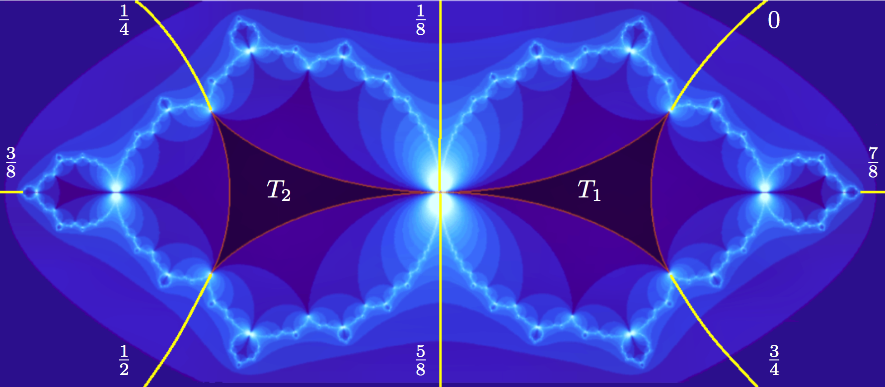
Figure 1. Illustrated is the mapping of Theorem A. The dynamical planes of Schwarz reflection maps of elements in Σ4∗\Sigma_{4}^{*} are illustrated next to the limit sets of the corresponding reflection groups in β⁡(𝚪5)\beta(\boldsymbol{\Gamma}_{5}). The top-left entry corresponds to the base points z↦z−1/(4​z4)z\mapsto z-1/(4z^{4}) and 𝚪5\boldsymbol{\Gamma}_{5} in Σ4∗\Sigma_{4}^{*}, β⁡(𝚪5)\beta(\boldsymbol{\Gamma}_{5}) respectively. The bottom-left and bottom-right dynamical planes lie on the boundary of the parameter spaces.

It is worth mentioning that the homeomorphism between the parameter spaces appearing in Theorem A has a geometric interpretation. To see this, let us first note that just like the group 𝚪d+1\boldsymbol{\Gamma}_{d+1} is a natural base point in its Bers compactification, the map f0​(z)=z−1/d​zdf_{0}(z)=z-1/dz^{d} can be seen as a base point of Σd∗\Sigma_{d}^{*}. In fact, the complement of f0​(𝔻∗)f_{0}(\mathbb{D}^{*}) is a (d+1)(d+1)-gon that is conformally isomorphic to the (closure of the) bounded part of the fundamental domain of 𝚪d+1\boldsymbol{\Gamma}_{d+1}. The pinching deformation technique for the family Σd∗\Sigma_{d}^{*}, as developed in [LMM19], then shows that all other members of Σd∗\Sigma_{d}^{*} can be obtained from f0f_{0} by quasiconformally deforming ℂ∖f0​(𝔻∗)\mathbb{C}\setminus f_{0}(\mathbb{D}^{*}) and letting various sides of this (d+1)(d+1)-gon touch. Analogously, all groups in β⁡(𝚪d+1)¯\overline{\beta(\boldsymbol{\Gamma}_{d+1})} can be obtained from 𝚪d+1\boldsymbol{\Gamma}_{d+1} by quasiconformally deforming the fundamental domain and letting the boundary circles touch (this also has the interpretation of pinching suitable geodesics on a (d+1)(d+1)-times punctured sphere). This suggests that one can define analogues of Fenchel-Nielsen coordinates on int⁡Σd∗\Int{\Sigma_{d}^{*}} and β⁡(𝚪d+1)\beta(\boldsymbol{\Gamma}_{d+1}) (the latter is just a real slice of the Teichmüller space of (d+1)(d+1)-times punctured spheres) using extremal lengths of path families connecting various sides of the corresponding (d+1)(d+1)-gons. The homeomorphism of Theorem A is geometric in the sense that it respects these coordinates on int⁡Σd∗\Int{\Sigma_{d}^{*}} and β⁡(𝚪d+1)\beta(\boldsymbol{\Gamma}_{d+1}) (compare the proof of Theorem 3.6).

We also note that the boundary of the Bers slice β⁡(𝚪d+1)\beta(\boldsymbol{\Gamma}_{d+1}) is considerably simpler than Bers slices of Fuchsian groups; more precisely, all groups on ∂β⁡(𝚪d+1)\partial\beta(\boldsymbol{\Gamma}_{d+1}) are geometrically finite (or equivalently, cusps), and are obtained by pinching a special collection of curves on a (d+1)(d+1)-times punctured sphere (see the last paragraph of Subsection 2.2). It is this feature of the Bers slices of reflection groups that is responsible for continuity of the dynamically defined map from Σd∗\Sigma_{d}^{*} to β⁡(𝚪d+1)¯\overline{\beta(\boldsymbol{\Gamma}_{d+1})}. This should be contrasted with the usual Fuchsian situation where the natural map from one Bers slice to another typically does not admit a continuous extension to the Bers boundaries (see [KT90]).

We now turn our attention to the other theme of the paper. This is related to the parallel notion of laminations that appears in the study of Kleinian groups and polynomial dynamics. The limit set of each group Γ\Gamma in β⁡(𝚪d+1)¯\overline{\beta(\boldsymbol{\Gamma}_{d+1})} is topologically modeled as the quotient of the limit set of 𝚪d+1\boldsymbol{\Gamma}_{d+1} by a geodesic lamination that is invariant under the reflection map ρ𝚪d+1\rho_{\boldsymbol{\Gamma}_{d+1}} (see Proposition 2.36 and Remark 4.25). Due to the existence of a topological conjugacy between ρ𝚪d+1\rho_{\boldsymbol{\Gamma}_{d+1}} and z¯d\overline{z}^{d}, this geodesic lamination can be “pushed forward” to obtain a z¯d\overline{z}^{d}-invariant equivalence relation on the unit circle (such equivalence relations are known as polynomial laminations in holomorphic dynamics). Using classical results from holomorphic dynamics, we show that this z¯d\overline{z}^{d}-invariant equivalence relation is realized as the lamination of the Julia set of a degree dd anti-polynomial. This leads to our second main result.

Theorem B.

Let Γ∈β⁡(𝚪d+1)¯\Gamma\in\overline{\beta(\boldsymbol{\Gamma}_{d+1})}. Then there exists a critically fixed anti-polynomial pp of degree dd such that the dynamical systems

ρΓ:Λ⁡(Γ)→Λ⁡(Γ),\displaystyle\rho_{\Gamma}:\Lambda(\Gamma)\rightarrow\Lambda(\Gamma),
p:𝒥⁡(p)→𝒥⁡(p)\displaystyle p:\mathcal{J}(p)\rightarrow\mathcal{J}(p)

are topologically conjugate.

We remark that the proof proceeds by showing that the systems in Theorem B are both topologically conjugate to the Schwarz reflection map of an appropriate element of Σd∗\Sigma_{d}^{*} acting on its limit set (see Theorem C). This implies, in particular, that all the three fractals; namely, the Julia set of the anti-polynomial pp, the limit set of the necklace group Γ\Gamma, and the limit set of the Schwarz reflection map of an appropriate element of Σd∗\Sigma_{d}^{*}, are homeomorphic. However, the incompatibility of the structures of cusp points on these fractals imply that they are not quasiconformally equivalent; i.e., there is no global quasiconformal map carrying one fractal to another (compare Figures 3, 6, and 8). Theorem B plays an important role in the recent work [LMMN20], where limit sets of necklace reflection groups are shown to be conformally removable. One of the main steps in the proof is to show that the topological conjugacy between p|𝒥⁡(p)p|_{\mathcal{J}(p)} and ρΓ|Λ⁡(Γ)\rho_{\Gamma}|_{\Lambda(\Gamma)} (provided by Theorem B) can be extended to a David homeomorphism of the sphere.

Let us now briefly outline the organization of the paper. Section 2 collects fundamental facts and known results about the objects studied in the paper. More precisely, in Subsection 2.1, we recall the definitions of the basic dynamical objects associated with the space Σd∗\Sigma_{d}^{*} of univalent rational maps. Subsection 2.2 introduces the class of reflection groups that will play a key role in the paper. Here we define the Bers slice β⁡(𝚪d)\beta(\boldsymbol{\Gamma}_{d}) of the regular ideal polygon reflection group 𝚪d\boldsymbol{\Gamma}_{d} (following the classical construction of Bers slices of Fuchsian groups), and describe its compactification β⁡(𝚪d)¯\overline{\beta(\boldsymbol{\Gamma}_{d})} in a suitable space of discrete, faithful representations. To each reflection group Γ∈β⁡(𝚪d)¯\Gamma\in\overline{\beta(\boldsymbol{\Gamma}_{d})}, we then associate the reflection map ρΓ\rho_{\Gamma} that is orbit equivalent to the group (this mimics a construction of Bowen and Series [BS79]). Using the reflection group ρΓ\rho_{\Gamma}, we formalize the notion of conformal mating of a reflection group and an anti-polynomial in Subsection 2.3. Section 3 proves half of Theorem A; here we prove that there is a natural homeomorphism between the spaces Σd∗\Sigma_{d}^{*} and β⁡(𝚪d)¯\overline{\beta(\boldsymbol{\Gamma}_{d})}. We should mention that the results of Section 3 depend on some facts about the space Σd∗\Sigma_{d}^{*} (and the associated Schwarz reflection maps) whose proofs are somewhat technical and hence deferred to Section 4. A recurring difficulty in our study is the unavailability of normal family arguments since Schwarz reflection maps are not defined on all of ℂ^\widehat{\mathbb{C}}. After proving some preliminary results about the topology of the limit set of a Schwarz reflection map arising from Σd∗\Sigma_{d}^{*} in Subsections 4.1 and 4.2, we proceed to the proofs of the statements about Σd∗\Sigma_{d}^{*} that are used in Section 3 (more precisely, Lemma 4.14, Proposition 4.19, and 4.20). The rest of Section 4 is devoted to the proof of the conformal mating statement of Theorem A. This completes the proof of our first main theorem. Finally, in Section 5, we use the theory of Hubbard trees for anti-holomorphic polynomials to prove Theorem B.

Acknowledgements. The third author was supported by an endowment from Infosys Foundation.

2. Preliminaries

Notation 2.1.

We denote by 𝔻∗\mathbb{D}^{*} the exterior unit disc ℂ^∖𝔻¯\widehat{\mathbb{C}}\setminus\overline{\mathbb{D}}. The Julia set of a holomorphic or anti-holomorphic polynomial p:ℂ^→ℂ^p:\widehat{\mathbb{C}}\rightarrow\widehat{\mathbb{C}} will be denoted by 𝒥⁡(p)\mathcal{J}(p), and its filled Julia set by 𝒦⁡(p)\mathcal{K}(p).

2.1. The Space Σd∗\Sigma_{d}^{*} and Schwarz Reflection Maps

Definition 2.2.

We will denote by Σd∗\Sigma_{d}^{*} the following class of rational maps:

Σd∗:={f⁡(z)=z+a1z+⋯+adzd:ad=−1d​ and ​f|𝔻∗​ is conformal.}.\Sigma_{d}^{*}:=\left\{f(z)=z+\frac{a_{1}}{z}+\cdots+\frac{a_{d}}{z^{d}}:a_{d}=-\frac{1}{d}\textrm{ and }f|_{\mathbb{D}^{*}}\textrm{ is conformal.}\right\}.

Note that for each d≥2d\geq 2, the space Σd∗\Sigma_{d}^{*} can be regarded as a slice of the space of schlicht functions:

Σ:={f⁡(z)=z+a1z+⋯+adzd+⋯:f|𝔻∗​ is conformal}.\Sigma:=\left\{f(z)=z+\frac{a_{1}}{z}+\cdots+\frac{a_{d}}{z^{d}}+\cdots:\ f|_{\mathbb{D}^{*}}\textrm{ is conformal}\right\}.

We endow Σd∗\Sigma_{d}^{*} with the topology of coefficient-wise convergence. Clearly, this topology is equivalent to that of uniform convergence on compact subsets of 𝔻∗\mathbb{D}^{*}.

Definition 2.3.

Given f∈Σd∗f\in\Sigma_{d}^{*}, we define the associated Schwarz reflection map σf:f⁡(𝔻∗)→ℂ^\sigma_{f}:f(\mathbb{D}^{*})\to\widehat{\mathbb{C}} by the following diagram:

𝔻∗{\lx@inpgf@ignorespaces\mathbb{D}^{*}}𝔻{\lx@inpgf@ignorespaces\mathbb{D}}f⁡(𝔻∗){\lx@inpgf@ignorespaces f(\mathbb{D}^{*})}ℂ^{\lx@inpgf@ignorespaces\widehat{\mathbb{C}}}z↦1/z¯\scriptstyle{\lx@inpgf@ignorespaces z\mapsto 1/\bar{z}}f\scriptstyle{\lx@inpgf@ignorespaces f}σf\scriptstyle{\lx@inpgf@ignorespaces\sigma_{f}}f−1\scriptstyle{\lx@inpgf@ignorespaces f^{-1}}

The map σf:σf−1​(f⁡(𝔻∗))→f⁡(𝔻∗)\sigma_{f}:\sigma_{f}^{-1}(f(\mathbb{D}^{*}))\to f(\mathbb{D}^{*}) is a proper branched covering map of degree dd (branched only at ∞\infty), and σf:σf−1​(int⁡f​(𝔻∗)c)→int⁡f​(𝔻∗)c\sigma_{f}:\sigma_{f}^{-1}(\Int{f(\mathbb{D}^{*})^{c}})\to\Int{f(\mathbb{D}^{*})^{c}} is a degree (d+1)(d+1) covering map.

We also note that ∞\infty is a super-attracting fixed point of σf\sigma_{f}; more precisely, ∞\infty is a fixed critical point of σf\sigma_{f} of multiplicity (d−1)(d-1).

Definition 2.4.

Let f∈Σd∗f\in\Sigma_{d}^{*}. We define the basin of infinity for σf\sigma_{f} as

ℬ∞​(σf):={z∈ℂ^:σf∘n​(z)→n→∞∞}.\mathcal{B}_{\infty}(\sigma_{f}):=\{z\in\widehat{\mathbb{C}}:\sigma_{f}^{\circ n}(z)\xrightarrow{n\rightarrow\infty}\infty\}.
Remark 2.5.

Let f∈Σd∗f\in\Sigma_{d}^{*}. Since σf\sigma_{f} has no critical point other than ∞\infty in ℬ∞​(σf)\mathcal{B}_{\infty}(\sigma_{f}), the proof of [Mil06, Theorem 9.3] may be adapted to show the existence of a Böttcher coordinate for σf\sigma_{f}: a conformal map

(1) ϕσf:𝔻∗→ℬ∞​(σf)​ such that ​ϕσf−1∘σf∘ϕσf​(u)=u¯d,∀u∈𝔻∗.\phi_{\sigma_{f}}:\mathbb{D}^{*}\rightarrow\mathcal{B}_{\infty}(\sigma_{f})\textrm{ such that }\phi_{\sigma_{f}}^{-1}\circ\sigma_{f}\circ\phi_{\sigma_{f}}(u)=\overline{u}^{d},\ \forall\ u\in\mathbb{D}^{*}.

Since

σf​(z)=−z¯dd+O⁡(z¯d−1)​as​z→∞,\sigma_{f}(z)=-\frac{\overline{z}^{d}}{d}+O(\overline{z}^{d-1})\ \textrm{as}\ z\to\infty,

we may choose ϕσf\phi_{\sigma_{f}} such that

(2) ϕσf′​(∞)=d1d−1​ei​πd+1.\displaystyle\phi_{\sigma_{f}}^{\prime}(\infty)=d^{\frac{1}{d-1}}e^{\frac{i\pi}{d+1}}.

As in [Mil06, Theorem 9.3], any Böttcher coordinate for σf\sigma_{f} is unique up to multiplication by a d+1std+1^{\textrm{st}} root of unity. Thus, (2) determines a unique Böttcher coordinate ϕσf\phi_{\sigma_{f}} which we will henceforth refer to as the Böttcher coordinate for σf\sigma_{f}.

The set ℂ^∖f⁡(𝔻∗)\widehat{\mathbb{C}}\setminus f(\mathbb{D}^{*}) is called the droplet, or fundamental tile, and is denoted by T⁡(σf)T(\sigma_{f}). By [LMM19, Proposition 2.8] and [LM14, Lemma 2.4], the curve ∂T=f⁡(𝕋)\partial T=f(\mathbb{T}) has (d+1)(d+1) distinct cusps and at most (d−2)(d-2) double points.The desingularized droplet To​(σf)T^{o}(\sigma_{f}) is defined as

To​(σf):=T⁡(σf)∖{ζ:ζ​ is a cusp or double point of ​f​(𝕋)}.T^{o}(\sigma_{f}):=T(\sigma_{f})\setminus\left\{\zeta:\zeta\textrm{ is a cusp or double point of }f(\mathbb{T})\right\}.
Definition 2.6.

The tiling set 𝒯∞​(σf)\mathcal{T}_{\infty}(\sigma_{f}) is defined as:

𝒯∞​(σf):=To​(σf)∪{z∈ℂ^:σf∘n​(z)∈To​(σf)​ for some ​n≥1}.\mathcal{T}_{\infty}(\sigma_{f}):=T^{o}(\sigma_{f})\cup\left\{z\in\widehat{\mathbb{C}}:\sigma_{f}^{\circ n}(z)\in T^{o}(\sigma_{f})\textrm{ for some }n\geq 1\right\}.

Lastly, we define the limit set of σf\sigma_{f} by Λ⁡(σf):=∂𝒯∞​(σf)\Lambda(\sigma_{f}):=\partial\mathcal{T}_{\infty}(\sigma_{f}).

For more details on the space Σd∗\Sigma_{d}^{*} and the associated Schwarz reflection maps, we refer the readers to [LMM19].

2.2. Reflection Groups and the Bers Slice

Notation 2.7.

We denote by Aut±​(ℂ^)\textrm{Aut}^{\pm}(\widehat{\mathbb{C}}) be the group of all Möbius and anti-Möbius automorphisms of ℂ^\widehat{\mathbb{C}}.

Definition 2.8.

A discrete subgroup Γ\Gamma of Aut±​(ℂ^)\textrm{Aut}^{\pm}(\widehat{\mathbb{C}}) is called a Kleinian reflection group if Γ\Gamma is generated by reflections in finitely many Euclidean circles.

Remark 2.9.

For a Euclidean circle CC, consider the upper hemisphere S⊂ℍ3:={(x,y,t)∈ℝ3:t>0}S\subset\mathbb{H}^{3}:=\{(x,y,t)\in\mathbb{R}^{3}:t>0\} such that ∂S∩∂ℍ3=C\partial S\cap\partial\mathbb{H}^{3}=C. Reflection in the Euclidean circle CC extends naturally to reflection in SS, and defines an orientation-reversing isometry of ℍ3\mathbb{H}^{3}. Hence, a Kleinian reflection Γ\Gamma group can be thought of as a 33-dimensional hyperbolic reflection group.

Since a Kleinian reflection group is discrete, by [VS93, Part II, Chapter 5, Proposition 1.4], we can choose its generators to be reflections in Euclidean circles C1,⋯,CdC_{1},\cdots,C_{d} such that:

(⋆\star) For each ​i​, the closure of the bounded component of ​ℂ^∖Ci​ does not contain any other ​Cj.\displaystyle\textrm{ For each }i\textrm{, the closure of the bounded component of }\widehat{\mathbb{C}}\setminus C_{i}\textrm{ does not contain any other }C_{j}.

We will always assume that a chosen generating set for a Kleinian reflection group Γ\Gamma satisfies Conditions (⋆\star).

Definition 2.10.

Let Γ\Gamma be a Kleinian reflection group. The domain of discontinuity of Γ\Gamma, denoted Ω⁡(Γ)\Omega(\Gamma), is the maximal open subset of ℂ^\widehat{\mathbb{C}} on which the elements of Γ\Gamma form a normal family. The limit set of Γ\Gamma, denoted by Λ⁡(Γ)\Lambda(\Gamma), is defined by Λ⁡(Γ):=ℂ^∖Ω⁡(Γ)\Lambda(\Gamma):=\widehat{\mathbb{C}}\setminus\Omega(\Gamma).

Refer to caption

Refer to caption

Figure 2. On the left is an interior necklace group, but the group generated by the circles pictured on the right violates condition (2) of Definition 2.11.

For a Euclidean circle CC, the bounded complementary component of CC will be called the interior of CC, and will be denoted by int⁡C\Int{C}.

Definition 2.11.

Let Γ\Gamma be a Kleinian reflection group. We say Γ\Gamma is a necklace group (see Figure 2) if it can be generated by reflections in Euclidean circles C1,⋯,CdC_{1},\cdots,C_{d} such that:

  1. (1)

    each circle CiC_{i} is tangent to Ci+1C_{i+1} (with i+1i+1 taken mod dd),

  2. (2)

    the boundary of the unbounded component of ℂ^∖∪iCi\widehat{\mathbb{C}}\setminus\cup_{i}C_{i} intersects each CiC_{i}, and

  3. (3)

    the circles CiC_{i} have pairwise disjoint interiors.

If, furthermore, Ci−1C_{i-1} and Ci+1C_{i+1} are the only circles to which any CiC_{i} is tangent, then Γ\Gamma is an interior necklace group.

Remark 2.12.

In Definition 2.11, Condition (2) ensures that each circle CiC_{i} is “seen” from ∞\infty - see Figure 2. When choosing a generating set for a necklace group, we always assume the generating set is chosen so as to satisfy Conditions (1)-(3), and the circles C1,⋯,CdC_{1},\cdots,C_{d} are labelled clockwise around ∞\infty. We note that a necklace group Γ\Gamma generated by reflections in dd Euclidean circles is isomorphic to the free product of dd copies of ℤ/2​ℤ\mathbb{Z}/2\mathbb{Z}.

Notation 2.13.

Given a necklace group Γ\Gamma with generating set given by reflections in circles C1,⋯,CdC_{1},\cdots,C_{d}, let

ℱΓ:=ℂ^∖(⋃i=1d(int⁡Ci∪{Cj∩Ci:j≠i})).\mathcal{F}_{\Gamma}:=\displaystyle\widehat{\mathbb{C}}\setminus\left(\bigcup_{i=1}^{d}(\Int{C_{i}}\cup\{C_{j}\cap C_{i}:j\not=i\})\right).
Proposition 2.14.

Let Γ\Gamma be a necklace group. Then ℱΓ\mathcal{F}_{\Gamma} is a fundamental domain for Γ\Gamma.

Proof.

Let 𝒫Γ\mathcal{P}_{\Gamma} be the convex hyperbolic polyhedron (in ℍ3\mathbb{H}^{3}) whose relative boundary in ℍ3\mathbb{H}^{3} is the union of the hyperplanes SiS_{i} (see Remark 2.9). Then, by [VS93, Part II, Chapter 5, Theorem 1.2], 𝒫Γ\mathcal{P}_{\Gamma} is a fundamental domain for the action of Γ\Gamma on ℍ3\mathbb{H}^{3}. It now follows that ℱΓ=𝒫Γ¯∩Ω⁡(Γ)\mathcal{F}_{\Gamma}=\overline{\mathcal{P}_{\Gamma}}\cap\Omega(\Gamma) (where the closure is taken in Ω⁡(Γ)∪ℍ3\Omega(\Gamma)\cup\mathbb{H}^{3}) is a fundamental domain for the action of Γ\Gamma on Ω⁡(Γ)\Omega(\Gamma) [Mar07, §3.5]. ∎

It will be useful in our discussion to have a canonical interior necklace group to refer to:

Definition 2.15.

Consider the Euclidean circles 𝐂1,⋯,𝐂d\mathbf{C}_{1},\cdots,\mathbf{C}_{d} where 𝐂j\mathbf{C}_{j} intersects |z|=1|z|=1 at right-angles at the roots of unity exp⁡(2​π​i⋅(j−1)d)\exp{(\frac{2\pi i\cdot(j-1)}{d})}, exp⁡(2​π​i⋅jd)\exp{(\frac{2\pi i\cdot j}{d})}. Let ρj\rho_{j} be the reflection map in the circle 𝐂j\mathbf{C}_{j}. By [VS93, Part II, Chapter 5, Theorem 1.2], this defines a necklace group

𝚪d:=⟨ρ1,⋯,ρd:ρ12=⋯=ρd2=1⟩,\boldsymbol{\Gamma}_{d}:=\langle\rho_{1},\cdots,\rho_{d}:\rho_{1}^{2}=\cdots=\rho_{d}^{2}=1\rangle,

that acts on the Riemann sphere.

Definition 2.16.

Let Γ\Gamma be a discrete subgroup of Aut±​(ℂ^)\textrm{Aut}^{\pm}(\widehat{\mathbb{C}}). An isomorphism

ξ:𝚪d→Γ\xi:\boldsymbol{\Gamma}_{d}\rightarrow\Gamma

is said to be weakly type-preserving, or w.t.p., if

  1. (1)

    ξ⁡(g)\xi(g) is orientation-preserving if and only if gg is orientation-preserving, and

  2. (2)

    ξ⁡(g)∈Γ\xi(g)\in\Gamma is a parabolic Möbius map for each parabolic Möbius map g∈𝚪dg\in\boldsymbol{\Gamma}_{d}.

In order to construct the Bers slice of the group 𝚪d\boldsymbol{\Gamma}_{d} and describe its compactification, we need to define a representation space for 𝚪d\boldsymbol{\Gamma}_{d}. For necklace groups, the information encoded by a representation (defined below) is equivalent to the data given by a labeling of the underlying circle packing. We will see in Section 3 that working with the space of representations (as opposed to the space of necklace groups without a labeling of the underlying circle packings) is crucial for the homeomorphism statement of Theorem A (compare Figure 5).

Definition 2.17.

We define

𝒟(𝚪d):={ξ:𝚪d→Γ|Γ is a discrete subgroup of Aut±(ℂ^), and ξ is a w.t.p. isomorphism}.\mathcal{D}(\boldsymbol{\Gamma}_{d}):=\{\xi:\boldsymbol{\Gamma}_{d}\to\Gamma|\ \Gamma\textrm{ is a discrete subgroup of }\textrm{Aut}^{\pm}(\widehat{\mathbb{C}}),\\ \textrm{ and }\xi\textrm{ is a w.t.p. isomorphism}\}.

We endow 𝒟⁡(𝚪d)\mathcal{D}(\boldsymbol{\Gamma}_{d}) with the topology of algebraic convergence: we say that a sequence (ξn)n=1∞⊂𝒟⁡(𝚪d)(\xi_{n})_{n=1}^{\infty}\subset\mathcal{D}(\boldsymbol{\Gamma}_{d}) converges to ξ∈𝒟⁡(𝚪d)\xi\in\mathcal{D}(\boldsymbol{\Gamma}_{d}) if ξn​(ρi)→ξ⁡(ρi)\xi_{n}(\rho_{i})\to\xi(\rho_{i}) coefficient-wise (as n→∞n\rightarrow\infty) for i=1,⋯,di=1,\cdots,d.

Remark 2.18.

Let ξ∈𝒟⁡(𝚪d)\xi\in\mathcal{D}(\boldsymbol{\Gamma}_{d}). Since for each i∈ℤ/d​ℤi\in\mathbb{Z}/d\mathbb{Z}, the Möbius map ρi∘ρi+1\rho_{i}\circ\rho_{i+1} is parabolic (this follows from the fact that each 𝐂i\mathbf{C}_{i} is tangent to 𝐂i+1\mathbf{C}_{i+1}), the w.t.p. condition implies that ξ⁡(ρi)∘ξ⁡(ρi+1)\xi(\rho_{i})\circ\xi(\rho_{i+1}) is also parabolic. As each ξ⁡(ρi)\xi(\rho_{i}) is an anti-conformal involution, it follows that ξ⁡(ρi)\xi(\rho_{i}) is Möbius conjugate to the circular reflection z↦1/z¯z\mapsto 1/\overline{z} or the antipodal map z↦−1/z¯z\mapsto-1/\overline{z}. A straightforward computation shows that the composition of −1/z¯-1/\overline{z} with either the reflection or the antipodal map with respect to any circle has two distinct fixed points in ℂ^\widehat{\mathbb{C}}, and hence not parabolic. Therefore, it follows that no ξ⁡(ρi)\xi(\rho_{i}) is Möbius conjugate to the antipodal map −1/z¯-1/\overline{z}. Hence, each ξ⁡(ρi)\xi(\rho_{i}) must be the reflection in some Euclidean circle CiC_{i}. Thus, Γ=ξ⁡(𝚪d)\Gamma=\xi(\boldsymbol{\Gamma}_{d}) is generated by reflections in the circles C1,⋯,CdC_{1},\cdots,C_{d}. The fact that ξ⁡(ρi)∘ξ⁡(ρi+1)\xi(\rho_{i})\circ\xi(\rho_{i+1}) is parabolic now translates to the condition that each CiC_{i} is tangent to Ci+1C_{i+1} (for i∈ℤ/d​ℤi\in\mathbb{Z}/d\mathbb{Z}). However, new tangencies among the circles CiC_{i} may arise. Moreover, that ξ\xi is an isomorphism rules out non-tangential intersection between circles CiC_{i}, CjC_{j} (indeed, a non-tangential intersection between CiC_{i} and CjC_{j} would introduce a new relation between ξ⁡(ρi)\xi(\rho_{i}) and ξ⁡(ρj)\xi(\rho_{j}), compare [VS93, Part II, Chapter 5, §1.1]). Therefore, Γ=ξ⁡(𝚪d)\Gamma=\xi(\boldsymbol{\Gamma}_{d}) is a Kleinian reflection group satisfying properties (1) and (3) of necklace groups.

Definition 2.19.

Let τ\tau be a conformal map defined in a neighborhood of ∞\infty with τ⁡(∞)=∞\tau(\infty)=\infty. We will say τ\tau is tangent to the identity at ∞\infty if τ′​(∞)=1\tau^{\prime}(\infty)=1. We will say τ\tau is hydrodynamically normalized if

τ⁡(z)=z+O⁡(1/z)​ as ​z→∞.\tau(z)=z+O(1/z)\textrm{ as }z\rightarrow\infty.
Definition 2.20.

Let Bel𝚪d\textrm{Bel}_{\boldsymbol{\Gamma}_{d}} denote those Beltrami coefficients μ\mu invariant under 𝚪d\boldsymbol{\Gamma}_{d}, satisfying μ=0\mu=0 a.e. on 𝔻∗\mathbb{D}^{*}. Let τμ:ℂ→ℂ\tau_{\mu}:\mathbb{C}\rightarrow\mathbb{C} denote the quasiconformal integrating map of μ\mu, with the hydrodynamical normalization. The Bers slice of Γ\Gamma is defined as

β(𝚪d):={ξ∈𝒟(𝚪d) | ξ(g)=τμ∘g∘τμ−1for allg∈𝚪d,whereμ∈Bel𝚪d}.\beta(\boldsymbol{\Gamma}_{d}):=\{\xi\in\mathcal{D}(\boldsymbol{\Gamma}_{d})\textrm{ | }\xi(g)=\tau_{\mu}\circ g\circ\tau_{\mu}^{-1}\ \textrm{for all}\ g\in\boldsymbol{\Gamma}_{d},\ \textrm{where}\ \mu\in\textrm{Bel}_{\boldsymbol{\Gamma}_{d}}\}.
Remark 2.21.

There is a natural free PSL2​(ℂ)\textrm{PSL}_{2}(\mathbb{C})-action on 𝒟⁡(𝚪d)\mathcal{D}(\boldsymbol{\Gamma}_{d}) given by conjugation, and so it is natural to consider the space AH​(𝚪d):=𝒟⁡(𝚪d)/PSL2​(ℂ)\textrm{AH}(\boldsymbol{\Gamma}_{d}):=\mathcal{D}(\boldsymbol{\Gamma}_{d})/\textrm{PSL}_{2}(\mathbb{C}). The following definition of the Bers slice, where no normalization for τμ\tau_{\mu} is specified, is more aligned with the classical Kleinian group literature:

(⋆\star) {ξ∈AH(𝚪d) | ξ(g)=τμ∘g∘τμ−1for allg∈𝚪d,whereμ∈Bel𝚪d}.\displaystyle\{\xi\in\textrm{AH}(\boldsymbol{\Gamma}_{d})\textrm{ | }\xi(g)=\tau_{\mu}\circ g\circ\tau_{\mu}^{-1}\ \textrm{for all}\ g\in\boldsymbol{\Gamma}_{d},\ \textrm{where}\ \mu\in\textrm{Bel}_{\boldsymbol{\Gamma}_{d}}\}.

Our Definition 2.20 of β⁡(𝚪d)\beta(\boldsymbol{\Gamma}_{d}) is simply a canonical choice of representative from each equivalence class of ( ⋆ ‣ 2.21), and will be more appropriate for the present work.

Lemma 2.22.

Let μ∈​B​e​l𝚪d\mu\in\emph{Bel}_{\boldsymbol{\Gamma}_{d}}, and τμ:ℂ→ℂ\tau_{\mu}:\mathbb{C}\rightarrow\mathbb{C} an integrating map. Then τμ∘𝚪d∘τμ−1\tau_{\mu}\circ\boldsymbol{\Gamma}_{d}\circ\tau_{\mu}^{-1} is a necklace group.

Proof.

By definition, the maps τμ∘ρi∘τμ−1\tau_{\mu}\circ\rho_{i}\circ\tau_{\mu}^{-1} generate the group τμ∘𝚪d∘τμ−1\tau_{\mu}\circ\boldsymbol{\Gamma}_{d}\circ\tau_{\mu}^{-1}. By invariance of μ\mu, each τμ∘ρi∘τμ−1\tau_{\mu}\circ\rho_{i}\circ\tau_{\mu}^{-1} is an anti-conformal involution of ℂ^\widehat{\mathbb{C}}, hence an anti-Möbius transformation. Since τμ∘ρi∘τμ−1\tau_{\mu}\circ\rho_{i}\circ\tau_{\mu}^{-1} fixes τμ​(Ci)\tau_{\mu}(C_{i}), and interchanges its two complementary components, it follows that τμ​(Ci)\tau_{\mu}(C_{i}) is a Euclidean circle and hence τμ∘ρi∘τμ−1\tau_{\mu}\circ\rho_{i}\circ\tau_{\mu}^{-1} is reflection in the circle τμ​(Ci)\tau_{\mu}(C_{i}). One readily verifies that the circles τμ​(Ci)\tau_{\mu}(C_{i}) satisfy the conditions of Definition 2.11, and so the result follows. ∎

Proposition 2.23.

The Bers slice β⁡(𝚪d)\beta(\boldsymbol{\Gamma}_{d}) is pre-compact in 𝒟⁡(𝚪d)\mathcal{D}(\boldsymbol{\Gamma}_{d}), and for each ξ∈β⁡(𝚪d)¯\xi\in\overline{\beta(\boldsymbol{\Gamma}_{d})}, the group ξ⁡(𝚪d)\xi(\boldsymbol{\Gamma}_{d}) is a necklace group.

Proof.

Let (ξn)n=1∞(\xi_{n})_{n=1}^{\infty} be a sequence in β⁡(𝚪d)\beta(\boldsymbol{\Gamma}_{d}), and τn:ℂ→ℂ\tau_{n}:\mathbb{C}\rightarrow\mathbb{C} the associated quasiconformal maps as in Definition 2.20. Since each τn\tau_{n} is conformal in 𝔻∗\mathbb{D}^{*} and is hydrodynamically normalized, by a standard normal family result (see [CG93, Theorem 1.10] for instance) there exists a conformal map τ∞\tau_{\infty} of 𝔻∗\mathbb{D}^{*} such that τn→τ∞\tau_{n}\rightarrow\tau_{\infty} uniformly on compact subsets of 𝔻∗\mathbb{D}^{*}, perhaps after passing to a subsequence which we reenumerate (τn)(\tau_{n}).

By Lemma 2.22, each τn​(𝐂i)\tau_{n}(\mathbf{C}_{i}) is a Euclidean circle which we denote by CinC_{i}^{n}. Since τn→τ∞\tau_{n}\rightarrow\tau_{\infty} uniformly on compact subsets of D∗D^{*}, τ∞​(Ci∩𝔻∗)\tau_{\infty}(C_{i}\cap\mathbb{D}^{*}) must be a subarc of a Euclidean circle which we denote by Ci∞C_{i}^{\infty}. Denote furthermore by ρin\rho_{i}^{n}, ρi∞\rho_{i}^{\infty} the reflections in the circles CinC_{i}^{n}, Ci∞C_{i}^{\infty} (respectively), and by Γ∞\Gamma_{\infty} the group generated by reflections in the circles (Ci∞)i=1d(C_{i}^{\infty})_{i=1}^{d}. Let ξ∞:𝚪d→Γ∞\xi_{\infty}:\boldsymbol{\Gamma}_{d}\rightarrow\Gamma_{\infty} be the homomorphism defined by ξ∞​(ρi):=ρi∞\xi_{\infty}(\rho_{i}):=\rho_{i}^{\infty}. We see that Cin→Ci∞C_{i}^{n}\rightarrow C_{i}^{\infty} as n→∞n\rightarrow\infty in the Hausdorff sense, whence it follows that ρin→ρi∞\rho_{i}^{n}\rightarrow\rho_{i}^{\infty}. This proves algebraic convergence (ξn)→ξ∞(\xi_{n})\rightarrow\xi_{\infty}. Hausdorff convergence of Cin→Ci∞C_{i}^{n}\rightarrow C_{i}^{\infty} also implies that each Ci∞C_{i}^{\infty} intersects tangentially with Ci+1∞C_{i+1}^{\infty}, so that ξ∞\xi_{\infty} is weakly type preserving. Similar considerations show that the circles Ci∞C_{i}^{\infty} have pairwise disjoint interiors, and the boundary of the unbounded component of ℂ^∖∪iCi∞\widehat{\mathbb{C}}\setminus\cup_{i}C_{i}^{\infty} intersects each Ci∞C_{i}^{\infty}. In particular, there cannot be any non-tangential intersection among the circles Ci∞C_{i}^{\infty}. It now follows that ξ∞\xi_{\infty} is indeed an isomorphism, and Γ∞=ξ∞​(𝚪d)\Gamma_{\infty}=\xi_{\infty}(\boldsymbol{\Gamma}_{d}) is a necklace group. ∎

Definition 2.24.

We refer to β⁡(𝚪d)¯⊂𝒟⁡(𝚪d)\overline{\beta(\boldsymbol{\Gamma}_{d})}\subset\mathcal{D}(\boldsymbol{\Gamma}_{d}) as the Bers compactification of the Bers slice β⁡(𝚪d)\beta(\boldsymbol{\Gamma}_{d}). We refer to β⁡(𝚪d)¯∖β⁡(𝚪d)\overline{\beta(\boldsymbol{\Gamma}_{d})}\setminus\beta(\boldsymbol{\Gamma}_{d}) as the Bers boundary.

Remark 2.25.

We will often identify ξ∈β⁡(𝚪d)¯\xi\in\overline{\beta(\boldsymbol{\Gamma}_{d})} with the group Γ:=ξ⁡(𝚪d)\Gamma:=\xi(\boldsymbol{\Gamma}_{d}), and simply write Γ∈β⁡(𝚪d)¯\Gamma\in\overline{\beta(\boldsymbol{\Gamma}_{d})}, but always with the understanding of an associated representation ξ:𝚪d→Γ\xi:\boldsymbol{\Gamma}_{d}\rightarrow\Gamma. Since ξ\xi is completely determined by its action on the generators ρ1,⋯,ρd\rho_{1},\cdots,\rho_{d} of 𝚪d\boldsymbol{\Gamma}_{d}, this is equivalent to remembering the ‘labeled’ circle packing C1,⋯,CdC_{1},\cdots,C_{d}, where ξ⁡(ρi)\xi(\rho_{i}) is reflection in the circle CiC_{i}, for i=1,⋯,di=1,\cdots,d.

Remark 2.26.

The Apollonian gasket reflection group (see the right-hand side of Figure 2) is an example of a Kleinian reflection group in 𝒟⁡(𝚪d)∖β⁡(𝚪d)¯\mathcal{D}(\boldsymbol{\Gamma}_{d})\setminus\overline{\beta(\boldsymbol{\Gamma}_{d})}.

Notation 2.27.

For Γ∈β⁡(𝚪d)¯\Gamma\in\overline{\beta(\boldsymbol{\Gamma}_{d})}, we denote the component of Ω⁡(Γ)\Omega(\Gamma) containing ∞\infty by Ω∞​(Γ)\Omega_{\infty}(\Gamma).

Proposition 2.28.

Let Γ∈β⁡(𝚪d)¯\Gamma\in\overline{\beta(\boldsymbol{\Gamma}_{d})}. Then the following hold true.

  1. (1)

    Ω∞​(Γ)\Omega_{\infty}(\Gamma) is simply connected, and Γ\Gamma-invariant.

  2. (2)

    ∂Ω∞​(Γ)=Λ⁡(Γ)\partial\Omega_{\infty}(\Gamma)=\Lambda(\Gamma).

  3. (3)

    Λ⁡(Γ)\Lambda(\Gamma) is connected, and locally connected.

  4. (4)

    All bounded components of Ω⁡(Γ)\Omega(\Gamma) are Jordan domains.

Proof.

1) It is evident from the construction of the Bers compactification that for each Γ∈β⁡(𝚪d)¯\Gamma\in\overline{\beta(\boldsymbol{\Gamma}_{d})}, there is a conformal map from 𝔻∗\mathbb{D}^{*} onto Ω∞​(Γ)\Omega_{\infty}(\Gamma) that conjugates the action of 𝚪d\boldsymbol{\Gamma}_{d} on 𝔻∗\mathbb{D}^{*} to that of Γ\Gamma on Ω∞​(Γ)\Omega_{\infty}(\Gamma). Hence, Ω∞​(Γ)\Omega_{\infty}(\Gamma) is simply connected, and invariant under Γ\Gamma.

2) This follows from (1) and the fact that the boundary of an invariant component of the domain of discontinuity is the entire limit set.

3) Connectedness of Λ⁡(Γ)\Lambda(\Gamma) follows from (2) and that Ω∞​(Γ)\Omega_{\infty}(\Gamma) is simply connected. For local connectivity, first note that the index two Kleinian subgroup Γ+\Gamma^{+} consisting of words of even length of Γ\Gamma is geometrically finite. Then Λ⁡(Γ)=Λ⁡(Γ+)\Lambda(\Gamma)=\Lambda(\Gamma^{+}), hence Λ⁡(Γ+)\Lambda(\Gamma^{+}) is connected. Since Γ+\Gamma^{+} is geometrically finite with a connected limit set, it now follows from [AM96] that Λ⁡(Γ+)=Λ⁡(Γ)\Lambda(\Gamma^{+})=\Lambda(\Gamma) is locally connected.

4) By (3), each component of Ω⁡(Γ)∖Ω∞​(Γ)\Omega(\Gamma)\setminus\Omega_{\infty}(\Gamma) is simply connected with a locally connected boundary. That such a component 𝒰\mathcal{U} is Jordan follows from the fact that ∂𝒰⊂Λ⁡(Γ)=∂Ω∞​(Γ)\partial\mathcal{U}\subset\Lambda(\Gamma)=\partial\Omega_{\infty}(\Gamma). ∎

To a group Γ∈β⁡(𝚪d)¯\Gamma\in\overline{\beta(\boldsymbol{\Gamma}_{d})}, we now associate a reflection map ρΓ\rho_{\Gamma} that will play an important role in the present work.

Definition 2.29.

Let Γ∈β⁡(𝚪d)¯\Gamma\in\overline{\beta(\boldsymbol{\Gamma}_{d})}, generated by reflections (ri)i=1d(r_{i})_{i=1}^{d} in circles (Ci)i=1d(C_{i})_{i=1}^{d}. We define the associated reflection map ρΓ\rho_{\Gamma} by:

ρΓ:⋃i=1dint​(Ci)¯→ℂ^\displaystyle\rho_{\Gamma}:\bigcup_{i=1}^{d}\overline{\textrm{int}(C_{i})}\rightarrow\widehat{\mathbb{C}}\hskip 48.36967pt
z⟼ri​(z)​ if ​z∈int​(Ci)¯.\displaystyle\hskip 28.45274ptz\longmapsto r_{i}(z)\textrm{ if }z\in\overline{\textrm{int}(C_{i})}.
Refer to captionRefer to captionint⁡C1\Int{C_{1}}int⁡C2\Int{C_{2}}int⁡C3\Int{C_{3}}int⁡C4\Int{C_{4}}ℱ\mathcal{F}ℱ\mathcal{F}ℱ\mathcal{F}Ω∞​(Γ)\Omega_{\infty}(\Gamma)
Figure 3. Left: The circles CiC_{i} generate a Kleinian reflection group Γ∈∂β⁡(𝚪4)\Gamma\in\partial\beta(\boldsymbol{\Gamma}_{4}). The map ρΓ\rho_{\Gamma} is defined piece-wise on the union of the closed disks int⁡Ci¯\overline{\Int{C_{i}}}. The fundamental domain ℱ=ℱΓ\mathcal{F}=\mathcal{F}_{\Gamma} (for the action of Γ\Gamma on Ω⁡(Γ)\Omega(\Gamma)) is the complement of these open disks with the singular boundary points removed. The connected components of ℱ\mathcal{F} are marked. Right: The unbounded component of the domain of discontinuity Ω⁡(Γ)\Omega(\Gamma) is Ω∞​(Γ)\Omega_{\infty}(\Gamma). Every point in Ω⁡(Γ)\Omega(\Gamma) escapes to ℱ\mathcal{F} under iterates of ρΓ\rho_{\Gamma}. The point of tangential intersection of C2C_{2} and C4C_{4} is the fixed point of an accidental parabolic of the index two Kleinian subgroup Γ~\widetilde{\Gamma}.
Definition 2.30.

Let Γ\Gamma be a Kleinian reflection group, and f:D→ℂ^f:D\rightarrow\widehat{\mathbb{C}} a mapping defined on a domain DD. We say that Γ\Gamma and ff are orbit-equivalent if for any two points z,w∈ℂ^z,w\in\widehat{\mathbb{C}}, there exists g∈Γg\in\Gamma with g⁡(z)=wg(z)=w if and only if there exist non-negative integers n1,n2n_{1},n_{2} such that f∘n1​(z)=f∘n2​(w)f^{\circ n_{1}}(z)=f^{\circ n_{2}}(w).

Proposition 2.31.

Let Γ∈β⁡(𝚪d)¯\Gamma\in\overline{\beta(\boldsymbol{\Gamma}_{d})}. The map ρΓ\rho_{\Gamma} is orbit equivalent to Γ\Gamma on ℂ^\widehat{\mathbb{C}}.

Proof.

Suppose z,w∈ℂ^z,w\in\widehat{\mathbb{C}} are such that there exist n1,n2∈ℕn_{1},n_{2}\in\mathbb{N} such that ρn1​(z)=ρn2​(w)\rho^{n_{1}}(z)=\rho^{n_{2}}(w). Since ρΓ\rho_{\Gamma} acts by the generators rir_{i} of the group Γ\Gamma, it follows directly that there exists g∈Γg\in\Gamma with g⁡(z)=wg(z)=w. Conversely, let z,w∈ℂ^z,w\in\widehat{\mathbb{C}} be such that there exists g∈Γg\in\Gamma with g⁡(z)=wg(z)=w. By definition, we have that g=rs1rs2⋯rsng=r_{s_{1}}r_{s_{2}}\cdots r_{s_{n}}, for some s1,⋯sn∈{1,⋯,d}s_{1},\cdots s_{n}\in\{1,\cdots,d\}. Suppose first that n=1n=1. Note that either zz or ww must belong to int⁡Cs1¯\overline{\Int{C_{s_{1}}}}. Since rs1​(z)=wr_{s_{1}}(z)=w implies rs1​(w)=zr_{s_{1}}(w)=z, there is no loss of generality in assuming that z∈int⁡Cs1¯z\in\overline{\Int{C_{s_{1}}}}. Now, the condition rs1​(z)=wr_{s_{1}}(z)=w can be written as ρΓ​(z)=w\rho_{\Gamma}(z)=w. The case n>1n>1 now follows by induction. ∎

Notation 2.32.

For Γ∈𝚪d¯\Gamma\in\overline{\boldsymbol{\Gamma}_{d}}, we will denote by To​(Γ)T^{o}(\Gamma) the union of all bounded components of the fundamental domain ℱΓ\mathcal{F}_{\Gamma} (see Proposition 2.14), and by Πo​(Γ)\Pi^{o}(\Gamma) the unique unbounded component of ℱΓ\mathcal{F}_{\Gamma}. We also set

T⁡(Γ):=To​(Γ)¯,and​Π​(Γ):=Πo​(Γ)¯.T(\Gamma):=\overline{T^{o}(\Gamma)},\ \textrm{and}\ \Pi(\Gamma):=\overline{\Pi^{o}(\Gamma)}.
Remark 2.33.

The set T⁡(Γ)T(\Gamma) should be thought of as the analogue of a droplet T⁡(σf)T(\sigma_{f}) (this analogy will become transparent in Proposition 3.2). On the other hand, the notation Π⁡(Γ)\Pi(\Gamma) is supposed to remind the readers that (the closure of) the unbounded component of ℱΓ\mathcal{F}_{\Gamma} is a “polygon."

Proposition 2.34.

Let Γ∈β⁡(𝚪d)¯\Gamma\in\overline{\beta(\boldsymbol{\Gamma}_{d})}. Then:

Ω⁡(Γ)=⋃n≥0ρΓ−n​(ℱΓ)​,a​n​d​Ω∞​(Γ)=⋃n≥0ρΓ−n​(Πo​(Γ)).\Omega(\Gamma)=\displaystyle\bigcup_{n\geq 0}\rho_{\Gamma}^{-n}(\mathcal{F}_{\Gamma})\emph{,and}\Omega_{\infty}(\Gamma)=\displaystyle\bigcup_{n\geq 0}\rho_{\Gamma}^{-n}(\Pi^{o}(\Gamma)).

In particular, Λ⁡(Γ)\Lambda(\Gamma) is completely invariant under ρΓ\rho_{\Gamma}.

Proof.

This follows from Propositions 2.14, 2.28, 2.31.∎

Remark 2.35.

Let Γ∈β⁡(𝚪d)¯\Gamma\in\overline{\beta(\boldsymbol{\Gamma}_{d})}. We now briefly describe the covering properties of ρΓ:Λ⁡(Γ)→Λ⁡(Γ)\rho_{\Gamma}:\Lambda(\Gamma)\to\Lambda(\Gamma). To this end, first note that

Λ⁡(Γ)=⋃i=1d(int⁡Ci¯∩Λ⁡(Γ))\Lambda(\Gamma)=\bigcup_{i=1}^{d}\left(\overline{\Int{C_{i}}}\cap\Lambda(\Gamma)\right)

(see Figure 3). The interiors of these dd “partition pieces” are disjoint, and ρΓ\rho_{\Gamma} maps each of them injectively onto the union of the others. This produces a Markov partition for the degree dd orientation-reversing covering map ρΓ:Λ⁡(Γ)→Λ⁡(Γ)\rho_{\Gamma}:\Lambda(\Gamma)\to\Lambda(\Gamma). In the particular case of the base group 𝚪d\boldsymbol{\Gamma}_{d}, the above discussion yields a Markov partition

𝕋=⋃j=1d[exp⁡(2​π​i​(j−1)d),exp⁡(2​π​i​jd)]\mathbb{T}=\displaystyle\bigcup_{j=1}^{d}\left[\exp{\left(\frac{2\pi i(j-1)}{d}\right)},\exp{\left(\frac{2\pi ij}{d}\right)}\right]

of the map ρ𝚪d:𝕋→𝕋\rho_{\boldsymbol{\Gamma}_{d}}:\mathbb{T}\to\mathbb{T}. Note that the expanding map

z¯d−1:𝕋→𝕋,\overline{z}^{d-1}:\mathbb{T}\to\mathbb{T},

or equivalently,

m−(d−1):ℝ/ℤ→ℝ/ℤ,θ↦−(d−1)​θm_{-(d-1)}:\mathbb{R}/\mathbb{Z}\to\mathbb{R}/\mathbb{Z},\ \theta\mapsto-(d-1)\theta

also admits the same Markov partition with the same transition matrix (identifying 𝕋\mathbb{T} with ℝ/ℤ\mathbb{R}/\mathbb{Z}). Following [LLMM18a, §3.2], one can define a homeomorphism

ℰd−1:𝕋→𝕋\mathcal{E}_{d-1}:\mathbb{T}\to\mathbb{T}

via the coding maps of ρ𝚪d|𝕋\rho_{\boldsymbol{\Gamma}_{d}}|_{\mathbb{T}} and z¯d−1|𝕋\overline{z}^{d-1}|_{\mathbb{T}} such that ℰd−1\mathcal{E}_{d-1} maps 11 to 11, and conjugates ρ𝚪d\rho_{\boldsymbol{\Gamma}_{d}} to z¯d−1\overline{z}^{d-1} (or m−(d−1)m_{-(d-1)}). Since both ρ𝚪d\rho_{\boldsymbol{\Gamma}_{d}} and z¯d−1\overline{z}^{d-1} commute with the complex conjugation map and ℰd−1\mathcal{E}_{d-1} fixes 11, one sees that ℰd−1\mathcal{E}_{d-1} commutes with the complex conjugation map as well.

The next result provides us with a model of the dynamics of ρΓ\rho_{\Gamma} on the limit set Λ⁡(Γ)\Lambda(\Gamma) as a quotient of the action of ρ𝚪d\rho_{\boldsymbol{\Gamma}_{d}} on the unit circle.

Proposition 2.36.

Let Γ∈β⁡(𝚪d)¯\Gamma\in\overline{\beta(\boldsymbol{\Gamma}_{d})}. There exists a conformal map ϕΓ:𝔻∗→Ω∞​(Γ)\phi_{\Gamma}:\mathbb{D}^{*}\rightarrow\Omega_{\infty}(\Gamma) such that

(3) ρ𝚪d​(z)=ϕΓ−1∘ρΓ∘ϕΓ​(z)​, for ​z∈𝔻∗∖int⁡Π⁡(𝚪d).\displaystyle\rho_{\boldsymbol{\Gamma}_{d}}(z)=\phi_{\Gamma}^{-1}\circ\rho_{\Gamma}\circ\phi_{\Gamma}(z)\textrm{, for }z\in\mathbb{D}^{*}\setminus\Int{\Pi(\boldsymbol{\Gamma}_{d})}.

The map ϕΓ\phi_{\Gamma} extends continuously to a semi-conjugacy ϕΓ:𝕋→Λ⁡(Γ)\phi_{\Gamma}:\mathbb{T}\rightarrow\Lambda(\Gamma) between ρ𝚪d|𝕋\rho_{\boldsymbol{\Gamma}_{d}}|_{\mathbb{T}} and ρΓ|Λ⁡(Γ)\rho_{\Gamma}|_{\Lambda(\Gamma)}, and ϕΓ\phi_{\Gamma} sends cusps of ∂Π⁡(𝚪d)\partial\Pi(\boldsymbol{\Gamma}_{d}) to cusps of ∂Π⁡(Γ)\partial\Pi(\Gamma) with labels preserved.

Proof.

Recall that 𝚪d\boldsymbol{\Gamma}_{d} is generated by reflections ρi\rho_{i} in circles (𝐂i)i=1d(\mathbf{C}_{i})_{i=1}^{d}. It follows from Propositions 2.14 and 2.28 that Πo​(𝚪d)\Pi^{o}(\boldsymbol{\Gamma}_{d}) and Πo​(Γ)\Pi^{o}(\Gamma) are fundamental domains for the actions of 𝚪d\boldsymbol{\Gamma}_{d} and Γ\Gamma on 𝔻∗\mathbb{D}^{*} and Ω∞​(Γ)\Omega_{\infty}(\Gamma), respectively. By the proofs of Lemma 2.22 and Proposition 2.23, there is a conformal mapping ϕΓ:int⁡Π⁡(𝚪d)→int⁡Π⁡(Γ)\phi_{\Gamma}:\Int{\Pi(\boldsymbol{\Gamma}_{d})}\rightarrow\Int{\Pi(\Gamma)} whose extension to ∂Π⁡(𝚪d)\partial\Pi(\boldsymbol{\Gamma}_{d}) is a label-preserving homeomorphism onto ∂Π⁡(Γ)\partial\Pi(\Gamma). Thus, by the Schwarz reflection principle, we may extend ϕΓ\phi_{\Gamma} to a conformal mapping ϕΓ:𝔻∗→Ω∞​(Γ)\phi_{\Gamma}:\mathbb{D}^{*}\rightarrow\Omega_{\infty}(\Gamma) which satisfies (3) by construction.

Note that ∂Ω∞​(Γ)=Λ⁡(Γ)\partial\Omega_{\infty}(\Gamma)=\Lambda(\Gamma). By local connectedness of Λ⁡(Γ)\Lambda(\Gamma) (see Proposition 2.28), the map ϕΓ\phi_{\Gamma} extends continuously to a semi-conjugacy 𝕋→Λ⁡(Γ)\mathbb{T}\rightarrow\Lambda(\Gamma). ∎

We will now introduce the notion of a label-preserving homeomorphism, which will play an important role in the proof of Theorem A.

Remark 2.37.

For f0​(z):=z−1/(d​zd)f_{0}(z):=z-1/(dz^{d}), label the non-zero critical points of f0f_{0} as ξ1f0,⋯,ξd+1f0\xi_{1}^{f_{0}},\cdots,\xi_{d+1}^{f_{0}} in counter-clockwise order with ξ1f0=ei​πd+1\xi_{1}^{f_{0}}=e^{\frac{i\pi}{d+1}}. Note that the critical points of ff vary continuously depending on f∈Σd∗f\in\Sigma_{d}^{*}, and f∈Σd∗f\in\Sigma_{d}^{*} can not have a double critical point on 𝕋\mathbb{T}. Since Σd∗\Sigma_{d}^{*} is connected by Proposition 4.19, there is a unique labeling ξ1f,⋯,ξd+1f\xi_{1}^{f},\cdots,\xi_{d+1}^{f} of critical points of any f∈Σd∗f\in\Sigma_{d}^{*} such that f↦ξiff\mapsto\xi_{i}^{f} is continuous (for i=1,⋯,d+1i=1,\cdots,d+1). This in turn determines a labeling of the cusps ζif:=f⁡(ξif)\zeta_{i}^{f}:=f(\xi_{i}^{f}) of f⁡(𝕋)f(\mathbb{T}) such that f↦ζiff\mapsto\zeta_{i}^{f} is continuous (i=1,⋯,d+1i=1,\cdots,d+1).

Similarly, label the cusps of ∂T⁡(𝚪d)\partial T(\boldsymbol{\Gamma}_{d}) as η1,⋯,ηd\eta_{1},\cdots,\eta_{d} in counter-clockwise order with η1=1\eta_{1}=1. This determines a labeling of cusps of ∂T⁡(Γ)\partial T(\Gamma) for any Γ∈β⁡(𝚪d)¯\Gamma\in\overline{\beta(\boldsymbol{\Gamma}_{d})} as the group Γ\Gamma is the image under a representation of 𝚪d\boldsymbol{\Gamma}_{d}.

Definition 2.38.

Let f∈Σd∗f\in\Sigma_{d}^{*} and Γ∈β⁡(𝚪d+1)¯\Gamma\in\overline{\beta(\boldsymbol{\Gamma}_{d+1})}. We say that a homeomorphism h:T⁡(Γ)→T⁡(σf)h:T(\Gamma)\rightarrow T(\sigma_{f}) is label-preserving if hh maps cusps of ∂T⁡(Γ)\partial T(\Gamma) to cusps of ∂T⁡(σf)\partial T(\sigma_{f}), and hh preserves the labeling of cusps of ∂T⁡(Γ)\partial T(\Gamma) and ∂T⁡(σf)\partial T(\sigma_{f}).

Similarly, for f,f′∈Σd∗f,f^{\prime}\in\Sigma_{d}^{*} (respectively, for Γ,Γ′∈β⁡(𝚪d+1)¯\Gamma,\Gamma^{\prime}\in\overline{\beta(\boldsymbol{\Gamma}_{d+1})}), a homeomorphism h:T⁡(σf)→T⁡(σf′)h:T(\sigma_{f})\rightarrow T(\sigma_{f^{\prime}}) (respectively, h:T⁡(Γ)→T⁡(Γ′)h:T(\Gamma)\rightarrow T(\Gamma^{\prime})) is called label-preserving if hh maps the boundary cusps to the boundary cusps preserving their labels.

We conclude this subsection with a discussion of the connection between the Bers slice of the reflection group 𝚪d\boldsymbol{\Gamma}_{d} and a classical Teichmüller space. Let 𝚪d+\boldsymbol{\Gamma}_{d}^{+} be the index two subgroup of 𝚪d\boldsymbol{\Gamma}_{d} consisting of all Möbius maps in 𝚪d\boldsymbol{\Gamma}_{d}. Then, 𝚪d+\boldsymbol{\Gamma}_{d}^{+} is Fuchsian group (it preserves 𝔻\mathbb{D} and 𝔻∗\mathbb{D}^{*}). Using Proposition 2.14, it is seen that the top and bottom surfaces S+:=𝔻∗/𝚪d+S^{+}:=\mathbb{D}^{*}/\boldsymbol{\Gamma}_{d}^{+} and S−:=𝔻/𝚪d+S^{-}:=\mathbb{D}/\boldsymbol{\Gamma}_{d}^{+} associated with the Fuchsian group 𝚪d+\boldsymbol{\Gamma}_{d}^{+} are dd times punctured spheres. Moreover, the anti-Möbius reflection ρi\rho_{i} in the circle 𝐂i\mathbf{C}_{i} descends to anti-conformal involutions on S±S^{\pm} fixing all the punctures (the resulting involution is independent of i∈{1,⋯,d}i\in\{1,\cdots,d\}). We will denote this involution on S−S^{-} by ι\iota.

By definition, each ξ∈𝒟⁡(𝚪d)\xi\in\mathcal{D}(\boldsymbol{\Gamma}_{d}) defines a discrete, faithful, w.t.p. representation of 𝚪d+\boldsymbol{\Gamma}_{d}^{+} into PSL2​(ℂ)\textrm{PSL}_{2}(\mathbb{C}). If ξ∈β⁡(𝚪d)\xi\in\beta(\boldsymbol{\Gamma}_{d}), then ξ\xi is induced by a quasiconformal map that is conformal on 𝔻∗\mathbb{D}^{*}. Hence, such a representation of 𝚪d+\boldsymbol{\Gamma}_{d}^{+} lies in the Bers slice of 𝚪d+\boldsymbol{\Gamma}_{d}^{+}. Thus, β⁡(𝚪d)\beta(\boldsymbol{\Gamma}_{d}) embeds into the Teichmüller space of a dd times punctured sphere.

On the other hand, each ξ∈β⁡(𝚪d)¯∖β⁡(𝚪d)\xi\in\overline{\beta(\boldsymbol{\Gamma}_{d})}\setminus\beta(\boldsymbol{\Gamma}_{d}) induces a representation of 𝚪d+\boldsymbol{\Gamma}_{d}^{+} that lies on the boundary of the Bers slice of the Fuchsian group 𝚪d+\boldsymbol{\Gamma}_{d}^{+}. The index two Kleinian group Γ+\Gamma^{+} of Γ:=ξ⁡(𝚪d)\Gamma:=\xi(\boldsymbol{\Gamma}_{d}) is geometrically finite (a fundamental polyhedron for the action of Γ+\Gamma^{+} on ℍ3\mathbb{H}^{3} is obtained by “doubling” a fundamental polyhedron for Γ\Gamma, and hence it has finitely many sides). In fact, Γ+\Gamma^{+} is a cusp group that is obtained by pinching a special collection of simple closed curves on S−S^{-}. Indeed, since S−S^{-} is equipped with a natural involution ι\iota, any 𝚪d\boldsymbol{\Gamma}_{d}-invariant Beltrami coefficient on 𝔻\mathbb{D} induces an ι\iota-invariant Beltrami coefficient on S−S^{-}. Hence, the simple closed geodesics on S−S^{-} that can be pinched via quasiconformal deformations with 𝚪d\boldsymbol{\Gamma}_{d}-invariant Beltrami coefficients are precisely the ones invariant under ι\iota. Moreover, the ι\iota-invariant simple closed geodesics on S−S^{-} bijectively correspond to pairs of non-tangential circles 𝐂i\mathbf{C}_{i} and 𝐂j\mathbf{C}_{j}; more precisely, they are the projections to S−S^{-} of hyperbolic geodesics of 𝔻\mathbb{D} with end-points at the two fixed points of the loxodromic Möbius map ρi∘ρj\rho_{i}\circ\rho_{j}. Hence, a group Γ+\Gamma^{+} on the Bers boundary is obtained as a limit of a sequence of quasiFuchsian deformations of 𝚪d+\boldsymbol{\Gamma}_{d}^{+} that pinch a disjoint union of ι\iota-invariant simple, closed, essential geodesics on the bottom surface S−S^{-} without changing the (marked) conformal equivalence class of the top surface S+S^{+}. If ξ⁡(ρi)\xi(\rho_{i}) is reflection in the circle CiC_{i} (for i=1,⋯,di=1,\cdots,d), then a point of intersection of some CiC_{i} and CjC_{j} with j≠i,i±1​(mod​d)j\neq i,i\pm 1\ (\textrm{mod}\ d) corresponds to an accidental parabolic ξ⁡(ρi∘ρj)\xi(\rho_{i}\circ\rho_{j}) for ξ⁡(𝚪d+)\xi(\boldsymbol{\Gamma}_{d}^{+}). Furthermore, the quotient

ℳ⁡(Γ+):=(ℍ3∪Ω⁡(Γ+))/Γ+\mathcal{M}(\Gamma^{+}):=\left(\mathbb{H}^{3}\cup\Omega(\Gamma^{+})\right)/\Gamma^{+}

is an infinite volume 33-manifold whose conformal boundary ∂ℳ⁡(Γ+):=Ω⁡(Γ+)/Γ+\partial\mathcal{M}(\Gamma^{+}):=\Omega(\Gamma^{+})/\Gamma^{+} consists of finitely many punctured spheres.

2.3. Conformal Mating

In this Subsection we define the notion of conformal mating in Theorem A. Our definitions follow [PM12], to which we refer for a more extensive discussion of conformal mating.

Notation 2.39.

For Γ∈β⁡(𝚪d)¯\Gamma\in\overline{\beta(\boldsymbol{\Gamma}_{d})}, recall Ω∞​(Γ)\Omega_{\infty}(\Gamma) denotes the unbounded component of Ω⁡(Γ)\Omega(\Gamma). We let 𝒦⁡(Γ):=ℂ∖Ω∞​(Γ)\mathcal{K}(\Gamma):=\mathbb{C}\setminus\Omega_{\infty}(\Gamma).

Remark 2.40.

Let w↦p⁡(w)w\mapsto p(w) be a monic, anti-holomorphic polynomial such that 𝒥⁡(p)\mathcal{J}(p) is connected and locally connected. Let d:=deg​(p)d:=\textrm{deg}(p), and denote by ϕp:𝔻∗→ℬ∞​(p)\phi_{p}:\mathbb{D}^{*}\rightarrow\mathcal{B}_{\infty}(p) the Böttcher coordinate for pp such that ϕp′​(∞)=1\phi_{p}^{\prime}(\infty)=1. We note that since ∂𝒦⁡(p)=𝒥⁡(p)\partial\mathcal{K}(p)=\mathcal{J}(p) is locally connected by assumption, it follows that ϕp\phi_{p} extends to a continuous semi-conjugacy between z↦z¯d|𝕋z\mapsto\overline{z}^{d}|_{\mathbb{T}} and p|𝒥⁡(p)p|_{\mathcal{J}(p)}. Now let Γ∈β⁡(𝚪d+1)¯\Gamma\in\overline{\beta(\boldsymbol{\Gamma}_{d+1})}. As was shown in Proposition 2.36, there is a natural continuous semi-conjugacy ϕΓ:𝕋→Λ⁡(Γ)\phi_{\Gamma}:\mathbb{T}\rightarrow\Lambda(\Gamma) between ρ𝚪d+1|𝕋\rho_{\boldsymbol{\Gamma}_{d+1}}|_{\mathbb{T}} and ρΓ|Λ⁡(Γ)\rho_{\Gamma}|_{\Lambda(\Gamma)}. Recall from Remark 2.35 that ℰd:𝕋→𝕋\mathcal{E}_{d}:\mathbb{T}\rightarrow\mathbb{T} is a topological conjugacy between ρ𝚪d+1|𝕋\rho_{\boldsymbol{\Gamma}_{d+1}}|_{\mathbb{T}} and z↦z¯d|𝕋z\mapsto\overline{z}^{d}|_{\mathbb{T}}.

Definition 2.41.

Let notation be as in Remark 2.40. We define an equivalence relation ∼\sim on 𝒦⁡(Γ)⊔𝒦⁡(p)\mathcal{K}(\Gamma)\sqcup\mathcal{K}(p) by specifying ∼\sim is generated by ϕΓ​(t)∼ϕp​(ℰd​(t)¯)\phi_{\Gamma}(t)\sim\phi_{p}(\overline{\mathcal{E}_{d}(t)}) for all t∈𝕋t\in\mathbb{T}.

Definition 2.42.

Let Γ∈β⁡(𝚪d+1)¯\Gamma\in\overline{\beta(\boldsymbol{\Gamma}_{d+1})}, pp a monic, anti-holomorphic polynomial such that 𝒥⁡(p)\mathcal{J}(p) is connected and locally connected, and f∈Σd∗f\in\Sigma_{d}^{*}. We say that σf\sigma_{f} is a conformal mating of Γ\Gamma with pp if there exist continuous maps

ψp:𝒦⁡(p)→ℂ^∖𝒯∞​(σf)​ and ​ψΓ:𝒦⁡(Γ)→𝒯∞​(σf)¯,\psi_{p}:\mathcal{K}(p)\rightarrow\widehat{\mathbb{C}}\setminus\mathcal{T}_{\infty}(\sigma_{f})\textrm{ and }\psi_{\Gamma}:\mathcal{K}(\Gamma)\rightarrow\overline{\mathcal{T}_{\infty}(\sigma_{f})},

conformal on int⁡𝒦⁡(p)\Int{\mathcal{K}(p)}, int⁡𝒦⁡(Γ)\Int{\mathcal{K}(\Gamma)}, respectively, such that

  1. (1)

    ψp∘p⁡(w)=σf∘ψp​(w)\psi_{p}\circ p(w)=\sigma_{f}\circ\psi_{p}(w) for w∈𝒦⁡(p)w\in\mathcal{K}(p),

  2. (2)

    ψΓ:T⁡(Γ)→T⁡(σf)\psi_{\Gamma}:T(\Gamma)\rightarrow T(\sigma_{f}) is label-preserving and ψΓ∘ρΓ​(z)=σf∘ψΓ​(z)\psi_{\Gamma}\circ\rho_{\Gamma}(z)=\sigma_{f}\circ\psi_{\Gamma}(z) for z∈𝒦⁡(Γ)∖int⁡To​(Γ)z\in\mathcal{K}(\Gamma)\setminus\Int{T^{o}(\Gamma)},

  3. (3)

    ψΓ​(z)=ψp​(w)​ if and only if ​z∼w\psi_{\Gamma}(z)=\psi_{p}(w)\textrm{ if and only if }z\sim w where ∼\sim is as in Definition 2.41.

2.4. Convergence of Quadrilaterals

We conclude Section 2 by recalling a notion of convergence for quadrilaterals (see [LV73, §I.4.9]) which will be useful to us in the proof of Theorem A. We will usually denote a topological quadrilateral by QQ, and its modulus by M⁡(Q)M(Q).

Definition 2.43.

The sequence of quadrilaterals QnQ_{n} (with a-sides aina_{i}^{n} and b-sides binb_{i}^{n}, i=1,2i=1,2, n∈ℕn\in\mathbb{N}) converges to the quadrilateral QQ (with a-sides aia_{i} and b-sides bib_{i}, i=1,2i=1,2) if to every ε>0\varepsilon>0 there corresponds an nεn_{\varepsilon} such that for n≥nεn\geq n_{\varepsilon}, every point of aina_{i}^{n}, binb_{i}^{n}, i=1,2i=1,2, and every interior point of QnQ_{n} has a spherical distance of at most ε\varepsilon from aia_{i}, bib_{i}, and QQ, respectively.

Theorem 2.44.

[LV73, §I.4.9] If the sequence of quadrilaterals QnQ_{n} converges to a quadrilateral QQ, then

limn→∞M⁡(Qn)=M⁡(Q).\lim_{n\rightarrow\infty}M(Q_{n})=M(Q).

3. A Homeomorphism Between Parameter Spaces

The purpose of this Section is to define the mapping in Theorem A and prove that it is a homeomorphism. We will prove the conformal mating statement in Theorem A in Section 4. First we will need the following rigidity result.

Proposition 3.1.

Let Γ\Gamma, Γ′\Gamma^{\prime} be necklace groups. Suppose there exist homeomorphisms

h1:T⁡(Γ)→T⁡(Γ′)​​a​n​d​h2:Π⁡(Γ)→Π⁡(Γ′)h_{1}:T(\Gamma)\rightarrow T(\Gamma^{\prime})\emph{and}h_{2}:\Pi(\Gamma)\rightarrow\Pi(\Gamma^{\prime})

which agree on cusps of ∂T⁡(Γ)\partial T(\Gamma), and map cusps of ∂T⁡(Γ)\partial T(\Gamma) to cusps of ∂T⁡(Γ′)\partial T(\Gamma^{\prime}). Suppose furthermore that h1h_{1}, h2h_{2} are conformal on To​(Γ′)T^{o}(\Gamma^{\prime}), Fo​(Γ′)F^{o}(\Gamma^{\prime}), respectively. Then h1h_{1}, h2h_{2} are restrictions of a common M∈​A​u​t​(ℂ)M\in\emph{Aut}(\mathbb{C}) such that

Γ′=M∘Γ∘M−1.\Gamma^{\prime}=M\circ\Gamma\circ M^{-1}.
Proof.

By iterated Schwarz reflection, we may extend the disjoint union of the maps h1h_{1}, h2h_{2} to a conformal isomorphism of the ordinary sets Ω⁡(Γ)\Omega(\Gamma), Ω⁡(Γ′)\Omega(\Gamma^{\prime}). Since Γ\Gamma, Γ′\Gamma^{\prime} are geometrically finite, the conclusion then follows from [Tuk85, Theorem 4.2]. ∎

Proposition 3.2.

Let f∈Σd∗f\in\Sigma_{d}^{*}. There exists a unique Γf∈β⁡(𝚪d+1)¯\Gamma_{f}\in\overline{\beta(\boldsymbol{\Gamma}_{d+1})} such that there is a label-preserving homeomorphism

h:T⁡(Γf)→T⁡(σf)h:T(\Gamma_{f})\rightarrow T(\sigma_{f})

with hh conformal on int T⁡(Γf)T(\Gamma_{f}).

Proof of Existence.

We first assume that f⁡(𝕋)f(\mathbb{T}) has no double points. Let

g:T⁡(𝚪d+1)→T⁡(σf)g:T(\boldsymbol{\Gamma}_{d+1})\rightarrow T(\sigma_{f})

be a label-preserving diffeomorphism such that

‖gz¯/gz‖L∞​(T⁡(𝚪d+1))<1.||g_{\overline{z}}/g_{z}||_{L^{\infty}(T(\boldsymbol{\Gamma}_{d+1}))}<1.

Define a Beltrami coefficient μg\mu_{g} by

μg​(u):=gz¯​(u)/gz​(u)​ for ​u∈T⁡(𝚪d+1),\mu_{g}(u):=g_{\overline{z}}(u)/g_{z}(u)\textrm{ for }u\in T(\boldsymbol{\Gamma}_{d+1}),

and

μg​(u):={μg​(ri∘n​(u)) if ​u∈ri−n​(T⁡(𝚪d+1))​ for ​1≤i≤d+1​ and ​n≥1,0otherwise.\mu_{g}(u):=\begin{cases}\mu_{g}(r_{i}^{\circ n}(u))&\textrm{ if }u\in r_{i}^{-n}(T(\boldsymbol{\Gamma}_{d+1}))\textrm{ for }1\leq i\leq d+1\textrm{ and }n\geq 1,\\ 0&\textrm{otherwise.}\end{cases}

Denote by τg:ℂ^→ℂ^\tau_{g}:\widehat{\mathbb{C}}\rightarrow\widehat{\mathbb{C}} the integrating map of μg\mu_{g}, normalized so that

τg​(z)=z+O⁡(1/|z|)​ as ​z→∞.\tau_{g}(z)=z+O(1/|z|)\textrm{ as }z\rightarrow\infty.

We claim that Γf:=τg∘𝚪d+1∘τg−1\Gamma_{f}:=\tau_{g}\circ\boldsymbol{\Gamma}_{d+1}\circ\tau_{g}^{-1} satisfies the conclusions of Proposition 3.2. Indeed,

τg∘𝚪d+1∘τg−1∈β⁡(𝚪d+1)\tau_{g}\circ\boldsymbol{\Gamma}_{d+1}\circ\tau_{g}^{-1}\in\beta({\boldsymbol{\Gamma}_{d+1}})

since μg≡0\mu_{g}\equiv 0 on 𝔻∗\mathbb{D}^{*}. The map

h:=g∘τg−1:T⁡(Γf)→T⁡(σf)h:=g\circ\tau_{g}^{-1}:T(\Gamma_{f})\rightarrow T(\sigma_{f})

is conformal on int ​TΓf\textrm{int }T_{\Gamma_{f}} since τg\tau_{g} is the integrating map for gz¯/gzg_{\overline{z}}/g_{z}. Lastly, we see that hh is label-preserving since τg−1\tau_{g}^{-1} and gg are both label-preserving by definition.

Next we consider the case that f⁡(𝕋)f(\mathbb{T}) has at least one double point. We claim the existence of Γ∈β⁡(𝚪d+1)¯\Gamma\in\overline{\beta(\boldsymbol{\Gamma}_{d+1})} such that there is a label-preserving diffeomorphism g:T⁡(Γ)→T⁡(σf).g:T(\Gamma)\rightarrow T(\sigma_{f}). Given the existence of such a Γ\Gamma, the same quasiconformal deformation argument as above produces the desired group Γf\Gamma_{f} and homeomorphism hh.

The existence of such a Γ\Gamma may be proven by pinching geodesics on the (d+1)(d+1)-times punctured sphere 𝔻/𝚪d+\mathbb{D}/\boldsymbol{\Gamma}_{d}^{+} (where 𝚪d+\boldsymbol{\Gamma}_{d}^{+} is the index 22 Kleinian subgroup of 𝚪d+1\boldsymbol{\Gamma}_{d+1} consisting of orientation-preserving automorphisms of ℂ\mathbb{C}), or adapting the techniques used in the proof of [LMM19, Theorem 4.11]. Alternatively, we may prove the existence of Γ\Gamma by associating a planar vertex viv_{i}, for 1≤i≤d+11\leq i\leq d+1, to each analytic arc connecting two cusps of f⁡(𝕋)f(\mathbb{T}), as in Figure 4. Connect two vertices viv_{i}, vjv_{j} by an edge if and only if the corresponding analytic arcs have non-empty intersection. This defines a simplicial 2-complex KK in the plane. KK is a combinatorial closed disc, and hence [Ste05, Proposition 6.1] shows that there is a circle packing (Ci′)i=1d+1(C_{i}^{\prime})_{i=1}^{d+1} of 𝔻\mathbb{D} for KK, with each Ci′C_{i}^{\prime} tangent to ∂𝔻\partial\mathbb{D}. Quasiconformally deforming this circle packing group so that there is a label-preserving conformal map to Π⁡(𝚪d+1)\Pi(\boldsymbol{\Gamma}_{d+1}) gives the desired Γ∈β⁡(𝚪d+1)¯\Gamma\in\overline{\beta(\boldsymbol{\Gamma}_{d+1})} (up to Möbius conjugacy). ∎

Refer to caption
Figure 4. Illustrated is the procedure of associating a circle packing to an element of Σd∗\Sigma_{d}^{*}.
Proof of Uniqueness.

If Γ\Gamma, Γ′\Gamma^{\prime} both satisfy the conclusions of the Proposition, we may take h1h_{1}, h2h_{2} as in Proposition 3.1, where h2​(z)=z+O⁡(1/z)h_{2}(z)=z+O(1/z) as z→∞z\rightarrow\infty since Γ\Gamma, Γ′∈β⁡(𝚪d+1)¯\Gamma^{\prime}\in\overline{\beta(\boldsymbol{\Gamma}_{d+1})}. Thus as h2h_{2} extends to an automorphism of ℂ\mathbb{C} by Proposition 3.1, it follows that h2=idh_{2}=\textrm{id}, and hence Γ=Γ′\Gamma=\Gamma^{\prime}. ∎

Remark 3.3.

The requirement that hh be label-preserving is essential to the uniqueness statement in the conclusion of Proposition 3.2: see Figure 5.

C1C_{1}C2C_{2}C3C_{3}C4C_{4}C3C_{3}C1C_{1}C4C_{4}C2C_{2}f⁡(𝕋)f(\mathbb{T})ζ1f\zeta_{1}^{f}ζ2f\zeta_{2}^{f}ζ3f\zeta_{3}^{f}ζ4f\zeta_{4}^{f}
Figure 5. Let f⁡(z):=z+t/z−1/(3​z3)∈Σ3∗f(z):=z+t/z-1/(3z^{3})\in\Sigma_{3}^{*} with t>0t>0. Then there are exactly two elements of β⁡(𝚪4)¯\overline{\beta(\boldsymbol{\Gamma}_{4})} whose corresponding interior fundamental domains are conformally isomorphic (with cusps preserved) to T⁡(σf)T(\sigma_{f}). However, only one of these conformal isomorphisms is label-preserving.
Proposition 3.4.

The mapping

(⋆\star) Σd∗→β⁡(𝚪d+1)¯\displaystyle\Sigma_{d}^{*}\rightarrow\overline{\beta(\boldsymbol{\Gamma}_{d+1})}
f↦Γf\displaystyle f\mapsto\Gamma_{f}\phantom{aasds}

defined in Proposition 3.2 is a bijection.

Proof.

We sketch a proof of surjectivity of ( ⋆ ‣ 3.4). Suppose first that Γ∈β⁡(𝚪d+1)¯\Gamma\in\overline{\beta(\boldsymbol{\Gamma}_{d+1})} is an interior necklace group, and let f0​(z):=z−1/(d​zd)∈Σd∗f_{0}(z):=z-1/(dz^{d})\in\Sigma_{d}^{*}. Pull back the standard conformal structure on To​(Γ)T^{o}(\Gamma) by a quasiconformal mapping 𝔥:T⁡(σf0)→To​(Γ)\mathfrak{h}:T(\sigma_{f_{0}})\rightarrow T^{o}(\Gamma) which preserves vertices, spread this conformal structure under the action of σf\sigma_{f} and extend elsewhere by the standard conformal structure, then straighten. This gives the desired element of Σd∗\Sigma_{d}^{*} which maps to Γ\Gamma (see the proof of [LMM19, Theorem 4.11] for details on quasiconformal deformations of ff). If Γ∈β⁡(𝚪d+1)¯\Gamma\in\overline{\beta(\boldsymbol{\Gamma}_{d+1})} is not an interior necklace group, Γ\Gamma still satisfies Condition (2) of Definition 2.11 by Proposition 2.23, and so by [LMM19, Theorem 4.11] there exists f∈Σd∗f\in\Sigma_{d}^{*} and a quasiconformal mapping 𝔥:T⁡(σf)→T⁡(Γ)\mathfrak{h}:T(\sigma_{f})\rightarrow T(\Gamma) preserving singularities, whence the above arguments apply.

We now show injectivity of ( ⋆ ‣ 3.4). Let ff, f′∈Σd∗f^{\prime}\in\Sigma_{d}^{*} such that Γf=Γf′\Gamma_{f}=\Gamma_{f^{\prime}}. Recall from Remark 2.5 that the Böttcher coordinates for σf\sigma_{f}, σf′\sigma_{f^{\prime}} are both tangent to z↦w​zz\mapsto wz at ∞\infty for the same ww. Thus there is a conjugacy Ψ\Psi between σf\sigma_{f}, σf′\sigma_{f^{\prime}} in a neighborhood of ∞\infty satisfying Ψ′​(∞)=1\Psi^{\prime}(\infty)=1. Since Γf=Γf′\Gamma_{f}=\Gamma_{f^{\prime}}, there is a label-preserving conformal isomorphism of T⁡(σf)→T⁡(σf′)T(\sigma_{f})\rightarrow T(\sigma_{f^{\prime}}), which defines Ψ\Psi in a finite part of the plane (disjoint from the neighborhood of ∞\infty in which Ψ\Psi is a conjugacy). Since the 00-rays for σf\sigma_{f}, σf′\sigma_{f^{\prime}} both land at a cusp with the same label (see Proposition 4.20), the definition of Ψ\Psi in the finite part of the plane and near ∞\infty can be connected along the 00-ray such that Ψ\Psi is a conjugacy along the 00-ray. The pullback argument of [LMM19, Theorem 5.1] now applies to show that Ψ\Psi is the restriction of a Möbius transformation MM. Since ff, f∈Σd∗f\in\Sigma_{d}^{*}, the map MM is multiplication by a d+1std+1^{\textrm{st}} root of unity. Since Ψ′​(∞)=1\Psi^{\prime}(\infty)=1, it follows that Ψ⁡(z)≡z\Psi(z)\equiv z. ∎

We now wish to show that the mapping of Proposition 3.4 is in fact a homeomorphism, for which we first need the following lemma:

Lemma 3.5.

Let UU, VV be Jordan domains. Let n≥4n\geq 4, and suppose u1,⋯,un∈∂Uu_{1},\cdots,u_{n}\in\partial U and v1,⋯,vn∈∂Vv_{1},\cdots,v_{n}\in\partial V are oriented positively with respect to UU, VV (respectively). Suppose furthermore that the quadrilaterals

U⁡(uj,uj+1,uk,uk+1),V⁡(vj,vj+1,vk,vk+1)U(u_{j},u_{j+1},u_{k},u_{k+1}),\hskip 11.38109ptV(v_{j},v_{j+1},v_{k},v_{k+1})

have the same modulus for each j,kj,k with 1≤j<j+2≤k≤n−11\leq j<j+2\leq k\leq n-1. Then there is a conformal map

f:U→V​ such that ​f​(ui)=vi​, ​1≤i≤n.f:U\rightarrow V\textrm{ such that }f(u_{i})=v_{i}\textrm{, }1\leq i\leq n.
Proof.

Let ΦU:U→𝔻\Phi_{U}:U\rightarrow\mathbb{D}, ΦV:V→𝔻\Phi_{V}:V\rightarrow\mathbb{D} be conformal maps such that

(4) ΦU​(uj)=ΦV​(vj)​ for ​1≤j≤3.\displaystyle\Phi_{U}(u_{j})=\Phi_{V}(v_{j})\textrm{ for }1\leq j\leq 3.

Suppose by way of contradiction that

(5) ΦU​(u4)≠ΦV​(v4).\displaystyle\Phi_{U}(u_{4})\not=\Phi_{V}(v_{4}).

Since U⁡(u1,u2,u3,u4)U(u_{1},u_{2},u_{3},u_{4}), V⁡(v1,v2,v3,v4)V(v_{1},v_{2},v_{3},v_{4}) have the same modulus, it follows that there is a conformal map g:U→Vg:U\rightarrow V with g⁡(uj)=vjg(u_{j})=v_{j} for 1≤j≤41\leq j\leq 4. But then

ΦV∘g∘ΦU−1:𝔻→𝔻\Phi_{V}\circ g\circ\Phi_{U}^{-1}:\mathbb{D}\rightarrow\mathbb{D}

is a Mobius transformation which fixes ΦU​(u1)\Phi_{U}(u_{1}), ΦU​(u2)\Phi_{U}(u_{2}), ΦU​(u3)∈∂𝔻\Phi_{U}(u_{3})\in\partial\mathbb{D} by (4), but is not the identity by (5), and this is a contradiction. This shows that

ΦU​(u4)=ΦV​(v4),\Phi_{U}(u_{4})=\Phi_{V}(v_{4}),

and the same argument applied recursively shows that

ΦU​(uj)=ΦV​(vj), for ​4≤j≤n.\Phi_{U}(u_{j})=\Phi_{V}(v_{j}),\textrm{ for }4\leq j\leq n.

The lemma follows by taking f=ΦV−1∘ΦUf=\Phi_{V}^{-1}\circ\Phi_{U}. ∎

Theorem 3.6.

The mapping

Σd∗→β⁡(𝚪d+1)¯\displaystyle\Sigma_{d}^{*}\rightarrow\overline{\beta(\boldsymbol{\Gamma}_{d+1})}
f↦Γf\displaystyle f\mapsto\Gamma_{f}\phantom{aasds}

defined in Proposition 3.2 is a homeomorphism.

Proof.

Let (fn)n=1∞∈Σd∗(f_{n})_{n=1}^{\infty}\in\Sigma_{d}^{*}, and suppose fn→f∞∈Σd∗f_{n}\rightarrow f_{\infty}\in\Sigma_{d}^{*}. We abbreviate Γn:=Γfn\Gamma_{n}:=\Gamma_{f_{n}}, Γ∞:=Γf∞\Gamma_{\infty}:=\Gamma_{f_{\infty}}. We want to show that

Γn→n→∞Γ∞​ in ​β⁡(𝚪d+1)¯.\Gamma_{n}\xrightarrow{n\rightarrow\infty}\Gamma_{\infty}\textrm{ in }\overline{\beta(\boldsymbol{\Gamma}_{d+1})}.

As β⁡(𝚪d+1)¯\overline{\beta(\boldsymbol{\Gamma}_{d+1})} is compact, we may assume, after passing to a subsequence, that Γn\Gamma_{n} converges to some Γ∞′∈β⁡(𝚪d+1)¯\Gamma_{\infty}^{\prime}\in\overline{\beta(\boldsymbol{\Gamma}_{d+1})}.

We denote the critical values of fnf_{n} by ζ1n,⋯,ζd+1n\zeta_{1}^{n},\cdots,\zeta_{d+1}^{n} (with the labeling chosen in Remark 2.37). For j,kj,k with 1≤j<j+2≤k≤d1\leq j<j+2\leq k\leq d, we consider the quadrilateral

Qn:=T⁡(σfn)​(ζjn,ζj+1n,ζkn,ζk+1n),Q_{n}:=T(\sigma_{f_{n}})(\zeta_{j}^{n},\zeta_{j+1}^{n},\zeta_{k}^{n},\zeta_{k+1}^{n}),

where we allow for the possibility that

(6)     ¿    ζjn​ζj+1n  ∩     ¿    ζkn​ζk+1n  ≠∅.\displaystyle\mathchoice{\vbox{\hbox{\resizebox{1869871}{0}{{\char 62\relax}}}\hbox{$\displaystyle\zeta_{j}^{n}\zeta_{j+1}^{n}$}}}{\vbox{\hbox{\resizebox{1869871}{0}{{\char 62\relax}}}\hbox{$\textstyle\zeta_{j}^{n}\zeta_{j+1}^{n}$}}}{\vbox{\hbox{\resizebox{1602975}{0}{{\char 62\relax}}}\hbox{$\scriptstyle\zeta_{j}^{n}\zeta_{j+1}^{n}$}}}{\vbox{\hbox{\resizebox{1562927}{0}{{\char 62\relax}}}\hbox{$\scriptscriptstyle\zeta_{j}^{n}\zeta_{j+1}^{n}$}}}\cap\mathchoice{\vbox{\hbox{\resizebox{1916179}{0}{{\char 62\relax}}}\hbox{$\displaystyle\zeta_{k}^{n}\zeta_{k+1}^{n}$}}}{\vbox{\hbox{\resizebox{1916179}{0}{{\char 62\relax}}}\hbox{$\textstyle\zeta_{k}^{n}\zeta_{k+1}^{n}$}}}{\vbox{\hbox{\resizebox{1644637}{0}{{\char 62\relax}}}\hbox{$\scriptstyle\zeta_{k}^{n}\zeta_{k+1}^{n}$}}}{\vbox{\hbox{\resizebox{1604589}{0}{{\char 62\relax}}}\hbox{$\scriptscriptstyle\zeta_{k}^{n}\zeta_{k+1}^{n}$}}}\not=\emptyset.

Note that the arcs in (6) may intersect in at most one point (see [LMM19, Proposition 4.8]), in which case we define

M⁡(Qn):=∞.\displaystyle M(Q_{n}):=\infty.

Similarly, if

(7)     ¿    ζj+1n​ζkn  ∩     ¿    ζk+1n​ζjn  ≠∅​, then ​M​(Qn):=0.\displaystyle\mathchoice{\vbox{\hbox{\resizebox{1869871}{0}{{\char 62\relax}}}\hbox{$\displaystyle\zeta_{j+1}^{n}\zeta_{k}^{n}$}}}{\vbox{\hbox{\resizebox{1869871}{0}{{\char 62\relax}}}\hbox{$\textstyle\zeta_{j+1}^{n}\zeta_{k}^{n}$}}}{\vbox{\hbox{\resizebox{1602975}{0}{{\char 62\relax}}}\hbox{$\scriptstyle\zeta_{j+1}^{n}\zeta_{k}^{n}$}}}{\vbox{\hbox{\resizebox{1562927}{0}{{\char 62\relax}}}\hbox{$\scriptscriptstyle\zeta_{j+1}^{n}\zeta_{k}^{n}$}}}\cap\mathchoice{\vbox{\hbox{\resizebox{1916179}{0}{{\char 62\relax}}}\hbox{$\displaystyle\zeta_{k+1}^{n}\zeta_{j}^{n}$}}}{\vbox{\hbox{\resizebox{1916179}{0}{{\char 62\relax}}}\hbox{$\textstyle\zeta_{k+1}^{n}\zeta_{j}^{n}$}}}{\vbox{\hbox{\resizebox{1644637}{0}{{\char 62\relax}}}\hbox{$\scriptstyle\zeta_{k+1}^{n}\zeta_{j}^{n}$}}}{\vbox{\hbox{\resizebox{1604589}{0}{{\char 62\relax}}}\hbox{$\scriptscriptstyle\zeta_{k+1}^{n}\zeta_{j}^{n}$}}}\not=\emptyset\textrm{, then }M(Q_{n}):=0.

We note that only one of (6) or (7) may occur (see [LMM19, Proposition 4.8]).

We also consider the quadrilaterals

Rn:=T⁡(Γn)​(hn−1​(ζjn),hn−1​(ζj+1n),hn−1​(ζkn),hn−1​(ζk+1n)),R_{n}:=T(\Gamma_{n})(h_{n}^{-1}(\zeta_{j}^{n}),h_{n}^{-1}(\zeta_{j+1}^{n}),h_{n}^{-1}(\zeta_{k}^{n}),h_{n}^{-1}(\zeta_{k+1}^{n})),

where

hn:Rn→Qnh_{n}:R_{n}\rightarrow Q_{n}

is a label-preserving conformal isomorphism by Proposition 3.2, so that

(8) M⁡(Qn)=M⁡(Rn)​ for all ​n.\displaystyle M(Q_{n})=M(R_{n})\textrm{ for all }n.

Since fn→f∞f_{n}\rightarrow f_{\infty} in Σd∗\Sigma_{d}^{*}, it follows from Theorem 2.44 that

(9) M⁡(Qn)→M⁡(Q∞)​ as ​n→∞.\displaystyle M(Q_{n})\rightarrow M(Q_{\infty})\textrm{ as }n\rightarrow\infty.

Now consider the quadrilateral

T⁡(Γ∞′)​(ηj∞,ηj+1∞,ηk∞,ηk+1∞),T(\Gamma_{\infty}^{\prime})(\eta_{j}^{\infty},\eta_{j+1}^{\infty},\eta_{k}^{\infty},\eta_{k+1}^{\infty}),

where ηj∞:=limnhn−1​(ζjn)\eta_{j}^{\infty}:=\lim_{n}h_{n}^{-1}(\zeta_{j}^{n}) is a cusp of T⁡(Γ∞′)T(\Gamma_{\infty}^{\prime}). Since Γn→Γ∞′\Gamma_{n}\rightarrow\Gamma_{\infty}^{\prime} in β⁡(𝚪d+1)¯\overline{\beta(\boldsymbol{\Gamma}_{d+1})}, it follows that

M⁡(Rn)→M⁡(T⁡(Γ∞′)​(ηj∞,ηj+1∞,ηk∞,ηk+1∞))​ as ​n→∞.M(R_{n})\rightarrow M(T(\Gamma_{\infty}^{\prime})(\eta_{j}^{\infty},\eta_{j+1}^{\infty},\eta_{k}^{\infty},\eta_{k+1}^{\infty}))\textrm{ as }n\rightarrow\infty.

Thus by (8) and (9),

M⁡(Q∞)=M⁡(T⁡(Γ∞′)​(ηj∞,ηj+1∞,ηk∞,ηk+1∞)).M(Q_{\infty})=M(T(\Gamma_{\infty}^{\prime})(\eta_{j}^{\infty},\eta_{j+1}^{\infty},\eta_{k}^{\infty},\eta_{k+1}^{\infty})).

As jj, kk are arbitrary, Lemma 3.5 applied to bounded components of ℂ∖f∞​(𝕋)\mathbb{C}\setminus f_{\infty}(\mathbb{T}) and int⁡T⁡(Γ∞′)\Int{T(\Gamma_{\infty}^{\prime})} yields a label-preserving conformal isomorphism

T⁡(Γ∞′)→T⁡(σf∞).T(\Gamma_{\infty}^{\prime})\rightarrow T(\sigma_{f_{\infty}}).

Thus by the uniqueness of Proposition 3.2, we have

Γ∞′=Γ∞,\Gamma_{\infty}^{\prime}=\Gamma_{\infty},

as needed. We conclude that

Σd∗→β⁡(𝚪d+1)¯\displaystyle\Sigma_{d}^{*}\rightarrow\overline{\beta(\boldsymbol{\Gamma}_{d+1})}
f↦Γf\displaystyle f\mapsto\Gamma_{f}\phantom{aasds}

is continuous, and the proof of continuity of the inverse is similar. ∎

4. Conformal Matings of Reflection groups and Polynomials

The purpose of Section 4 is to prove the conformal mating statement of Theorem A. In Section 4.1 we will show that ∂ℬ∞​(σf)\partial\mathcal{B}_{\infty}(\sigma_{f}) is locally connected for f∈Σd∗f\in\Sigma_{d}^{*}, whence in Section 4.2 we will show that ℬ∞​(σf)\mathcal{B}_{\infty}(\sigma_{f}) and 𝒯∞​(σf)\mathcal{T}_{\infty}(\sigma_{f}) share a common boundary. Sections 4.3 and 4.4 study laminations of 𝕋\mathbb{T} induced by σf\sigma_{f} and necklace groups Γ\Gamma, whence it is shown in Section 4.5 that for f∈Σd∗f\in\Sigma_{d}^{*}, the laminations induced by σf\sigma_{f} and Γf\Gamma_{f} are compatible. Finally, in Section 4.6, we deduce that σf\sigma_{f} is a conformal mating of Γf\Gamma_{f} and w↦w¯dw\mapsto\overline{w}^{d} (see Definition 2.42).

4.1. Local Connectivity

Lemma 4.1.

Let f∈Σd∗f\in\Sigma_{d}^{*}. Then

|∂¯​σf​(z)|>1​, ​∀z∈f⁡(𝔻∗).\left|\overline{\partial}\sigma_{f}(z)\right|>1\textrm{, }\forall z\in f(\mathbb{D}^{*}).
Proof.

Let σ:=σf\sigma:=\sigma_{f}. From Definition 2.3, we see that

(10) σ⁡(f⁡(w))=f⁡(1/w¯)​, for ​|w|>1.\sigma(f(w))=f\left(1/\overline{w}\right)\textrm{, for }|w|>1.

Taking the ∂¯\overline{\partial}-derivative of (10) yields

(11) ∂¯σ(f(w))⋅f′​(w)¯=−1w¯2⋅f′(1w¯),for|w|>1.\overline{\partial}\sigma\left(f(w)\right)\cdot\overline{f^{\prime}(w)}=-\frac{1}{\overline{w}^{2}}\cdot f^{\prime}\left(\frac{1}{\overline{w}}\right),\ \textrm{for}\ |w|>1.

By [LM14, Lemma 2.6], we also have that

(12) f′​(1w¯)=w¯d+1​f′​(w)¯,∀w∈ℂ.f^{\prime}\left(\frac{1}{\overline{w}}\right)=\overline{w}^{d+1}\overline{f^{\prime}(w)},\ \forall w\in\mathbb{C}.

Combining (11) and (12), we conclude that

|∂¯​σ​(f⁡(w))|=|w|d−1>1​ for ​|w|>1.|\overline{\partial}\sigma(f(w))|=|w|^{d-1}>1\textrm{ for }|w|>1.

∎

Proposition 4.2.

Let f∈Σd∗f\in\Sigma_{d}^{*}. Then ∂ℬ∞​(σf)\partial\mathcal{B}_{\infty}(\sigma_{f}) is locally connected.

Remark 4.3.

Our proof follows the strategy taken in [DH85, Chapter 10].

Proof.

Let σ:=σf\sigma:=\sigma_{f}, ϕσ:=ϕσf\phi_{\sigma}:=\phi_{\sigma_{f}} be as in Remark 2.5, and X:=ℬ∞​(σ)∩ℂX:=\mathcal{B}_{\infty}(\sigma)\cap\mathbb{C}. Note that σ:X→X\sigma:X\rightarrow X is a d:1d\hskip-2.84526pt:\hskip-2.84526pt1 covering map. Define an equipotential curve

E⁡(r):=ϕσ​({z∈ℂ:|z|=r}).E(r):=\phi_{\sigma}\left(\{z\in\mathbb{C}:|z|=r\}\right).

We define, for n≥1n\geq 1, parametrizations γn:𝕋→E⁡(21/dn)\gamma_{n}:\mathbb{T}\rightarrow E(2^{1/d^{n}}) by:

γn​(e2​π​i​θ):=ϕσ​(21/dn​e2​π​i​θ).\gamma_{n}(e^{2\pi i\theta}):=\phi_{\sigma}(2^{1/d^{n}}e^{2\pi i\theta}).

By (1), we have:

σ∘γn+1​(e2​π​i​θ)=γn​(e−2​π​i​d​θ).\sigma\circ\gamma_{n+1}(e^{2\pi i\theta})=\gamma_{n}(e^{-2\pi id\theta}).

We will show that the sequence (γn)n=1∞(\gamma_{n})_{n=1}^{\infty} forms a Cauchy sequence in the complete metric space C⁡(𝕋,ℂ)C(\mathbb{T},\mathbb{C}). We will denote the length of a curve γ\gamma by l⁡(γ)l(\gamma), and the lift of γ\gamma under σ\sigma by γ~\widetilde{\gamma}.

To this end, define h:ℝ≥0→ℝ≥0h:\mathbb{R}_{\geq 0}\rightarrow\mathbb{R}_{\geq 0} by

(13) h⁡(s):=supγ∈C⁡(𝕋,X)l⁡(γ)≤s{l⁡(γ~):σ⁡(γ~)=γ}.h(s):=\sup_{\begin{subarray}{c}\gamma\in C(\mathbb{T},X)\\ l(\gamma)\leq s\end{subarray}}\left\{l(\widetilde{\gamma}):\sigma(\widetilde{\gamma})=\gamma\right\}.

We claim that

(14) h⁡(s)<s​ and ​h​(k​s)≤k​h​(s)​, ​∀s>0​ and ​k∈ℕ.h(s)<s\textrm{ and }h(ks)\leq kh(s)\textrm{, }\forall s>0\textrm{ and }k\in\mathbb{N}.

Indeed, the first inequality of (14) follows from Lemma 4.1. The second inequality in (14) follows from the triangle inequality. It follows from (14) that s−h⁡(s)→∞s-h(s)\rightarrow\infty as s→∞s\rightarrow\infty. Let ℓ:=dist⁡(γ0,γ1)\ell:=\dist(\gamma_{0},\gamma_{1}), and choose L>ℓL>\ell sufficiently large such that L−h⁡(L)>ℓL-h(L)>\ell. One has:

dist⁡(γ2,γ0)≤dist⁡(γ2,γ1)+dist⁡(γ1,γ0)≤h⁡(ℓ)+ℓ≤h⁡(L)+ℓ<L.\dist(\gamma_{2},\gamma_{0})\leq\dist(\gamma_{2},\gamma_{1})+\dist(\gamma_{1},\gamma_{0})\leq h(\ell)+\ell\leq h(L)+\ell<L.

Similarly, an inductive procedure yields

dist⁡(γn,γ0)<L​, ​∀n≥0.\dist(\gamma_{n},\gamma_{0})<L\textrm{, }\forall n\geq 0.

Observe that

dist⁡(γn,γn+p)≤h∘n​(dist⁡(γ0,γp))<h∘n​(L).\dist(\gamma_{n},\gamma_{n+p})\leq h^{\circ n}(\dist(\gamma_{0},\gamma_{p}))<h^{\circ n}(L).

The sequence (h∘n​(L))n=1∞∈ℝ≥0(h^{\circ n}(L))_{n=1}^{\infty}\in\mathbb{R}_{\geq 0} is decreasing and converges to a fixpoint of hh, and this fixpoint must be 00 by (14). Thus (γn)n=1∞(\gamma_{n})_{n=1}^{\infty} is a Cauchy sequence, and the limit is a continuous extension of

ϕσ:𝔻∗→ℬ∞​(σ)​ to ​ϕσ:𝕋→∂ℬ∞​(σ).\phi_{\sigma}:\mathbb{D}^{*}\rightarrow\mathcal{B}_{\infty}(\sigma)\textrm{ to }\phi_{\sigma}:\mathbb{T}\rightarrow\partial\mathcal{B}_{\infty}(\sigma).

Local connectivity of ∂ℬ∞​(σ)\partial\mathcal{B}_{\infty}(\sigma) follows from a theorem of Carathéodory. ∎

4.2. The Limit Set is The Boundary of The Basin of Infinity

The goal of this Subsection is to prove the following:

Proposition 4.4.

Let f∈Σd∗f\in\Sigma_{d}^{*}. Then ∂ℬ∞​(σf)=∂𝒯∞​(σf)\partial\mathcal{B}_{\infty}(\sigma_{f})=\partial\mathcal{T}_{\infty}(\sigma_{f}).

The proof of Proposition 4.4 will be carried out by way of several lemmas below. First we record the following definition:

Definition 4.5.

Let f∈Σd∗f\in\Sigma_{d}^{*}. An external ray for σf\sigma_{f} is a curve

t↦ϕσf​(t​ei​θ)​, ​t∈(1,∞)t\mapsto\phi_{\sigma_{f}}(te^{i\theta})\textrm{, }t\in(1,\infty)

for some θ∈[0,2​π)\theta\in[0,2\pi), where ϕσf\phi_{\sigma_{f}} is the Böttcher coordinate of Remark 2.5. For θ∈[0,2​π)\theta\in[0,2\pi), we refer to

{ϕσf​(t​ei​θ):t∈(1,∞)}\{\phi_{\sigma_{f}}(te^{i\theta}):t\in(1,\infty)\}

as the θ\theta-ray of σf\sigma_{f}.

Remark 4.6.

By Proposition 4.2, each external ray of σf\sigma_{f} lands, in other words limt→1+ϕσf​(t​ei​θ)\lim_{t\rightarrow 1^{+}}\phi_{\sigma_{f}}(te^{i\theta}) exists for each θ∈[0,2​π)\theta\in[0,2\pi).

Notation 4.7.

Let Σd,k∗\Sigma_{d,k}^{*} denote the collection of those f∈Σd∗f\in\Sigma_{d}^{*} such that f⁡(𝕋)f(\mathbb{T}) has exactly kk double points.

For the remainder of this subsection we fix f∈Σd,k∗f\in\Sigma_{d,k}^{*} and denote σ:=σf\sigma:=\sigma_{f}. Let us first record the straightforward inclusion:

Lemma 4.8.

∂ℬ∞​(σ)⊂∂𝒯∞​(σ)\partial\mathcal{B}_{\infty}(\sigma)\subset\partial\mathcal{T}_{\infty}(\sigma).

Proof.

We note that 𝒯∞​(σ)\mathcal{T}_{\infty}(\sigma) is open, whence the relation

(15) ℂ^=𝒯∞​(σ)⊔∂𝒯∞​(σ)⊔ℬ∞​(σ)\displaystyle\widehat{\mathbb{C}}=\mathcal{T}_{\infty}(\sigma)\sqcup\partial\mathcal{T}_{\infty}(\sigma)\sqcup\mathcal{B}_{\infty}(\sigma)

follows from the classical classification of periodic Fatou components and the observation that σ\sigma has only one singular value (at ∞\infty). The Lemma follows from (15). ∎

The proof of the opposite inclusion is a bit more involved, and we split the main arguments into a couple of lemmas.

Lemma 4.9.

The landing points of the fixed external rays of σ\sigma are singular points of f⁡(𝕋)f(\mathbb{T}).

Proof.

Note that the landing points of the fixed rays of σ\sigma are necessarily fixed points of σ\sigma on ∂ℬ∞​(σ)\partial\mathcal{B}_{\infty}(\sigma). Since ∂ℬ∞​(σ)⊂∂𝒯∞​(σ)\partial\mathcal{B}_{\infty}(\sigma)\subset\partial\mathcal{T}_{\infty}(\sigma) by Lemma 4.8, the result will follow if we can prove that the only fixed points of σ|∂𝒯∞​(σ)\sigma|_{\partial\mathcal{T}_{\infty}(\sigma)} are the singular points of f⁡(𝕋)f(\mathbb{T}). This will be shown via the Lefschetz fixed-point formula.

As ff has kk double points, there are k+1k+1 forward-invariant components 𝒰1,⋯,𝒰k+1\mathcal{U}_{1},\cdots,\mathcal{U}_{k+1} of 𝒯∞​(σ)\mathcal{T}_{\infty}(\sigma), each containing a single component of To​(σ)T^{o}(\sigma). Let Ti:=𝒰i∩To​(σ)T_{i}:=\mathcal{U}_{i}\cap T^{o}(\sigma), so that TiT_{i} is naturally a (3+ji)(3+j_{i})-gon (ji≥0j_{i}\geq 0) whose vertices are the 3+ji3+j_{i} singularities of f⁡(𝕋)f(\mathbb{T}) lying on ∂𝒰i\partial\mathcal{U}_{i}. Each 𝒰i\mathcal{U}_{i} is a simply connected domain as it can be written as an increasing union of pullbacks (under σ\sigma) of TiT_{i} (see also [LLMM18a, Proposition 5.6]). Moreover, we can map each TiT_{i} conformally to a (3+ji)(3+j_{i})-gon in 𝔻\mathbb{D} whose edges are geodesics of 𝔻\mathbb{D}. By iterated Schwarz reflection, one now obtains a Riemann map from 𝔻\mathbb{D} onto 𝒰i\mathcal{U}_{i}. Using Lemma 4.1, one can mimic the proof of Proposition 4.2 to show that each ∂𝒰i\partial\mathcal{U}_{i} is locally connected.

We now consider a quasiconformal homeomorphism χi:To​(𝚪3+ji)→Ti\chi_{i}:T^{o}(\boldsymbol{\Gamma}_{3+j_{i}})\to T_{i} that sends the boundary cusps to the boundary cusps. Lifting χi\chi_{i} by ρ𝚪3+ji\rho_{\boldsymbol{\Gamma}_{3+j_{i}}} and σ\sigma, we obtain a quasiconformal homeomorphism χi:𝔻→𝒰i\chi_{i}:\mathbb{D}\to\mathcal{U}_{i} that conjugates ρ𝚪3+ji\rho_{\boldsymbol{\Gamma}_{3+j_{i}}} to σ\sigma. Since ∂𝒰i\partial\mathcal{U}_{i} is locally connected, χi\chi_{i} extends continuously to the boundary, and yields a topological semi-conjugacy between ρ𝚪3+ji|𝕋\rho_{\boldsymbol{\Gamma}_{3+j_{i}}}|_{\mathbb{T}} and σ|∂𝒰i\sigma|_{\partial\mathcal{U}_{i}}. It now follows from Remark 2.35 that

χ^i:=χi∘ℰ2+ji−1:𝕋→∂𝒰i\widehat{\chi}_{i}:=\chi_{i}\circ\mathcal{E}_{2+j_{i}}^{-1}:\mathbb{T}\to\partial\mathcal{U}_{i}

is a topological semi-conjugacy between z¯2+ji|𝕋\overline{z}^{2+j_{i}}|_{\mathbb{T}} and σ|∂𝒰i\sigma|_{\partial\mathcal{U}_{i}}. Let χ^i:𝔻¯→𝒰i¯\widehat{\chi}_{i}:\overline{\mathbb{D}}\to\overline{\mathcal{U}_{i}} be an arbitrary continuous extension of χ^i|𝕋\widehat{\chi}_{i}|_{\mathbb{T}} such that χ^i\widehat{\chi}_{i} maps 𝔻\mathbb{D} homeomorphically onto 𝒰i\mathcal{U}_{i}.

We now (topologically) glue attracting basins into the domains 𝒰i\mathcal{U}_{i}:

σˇ​(w):={σ⁡(w)on​ℂ^∖⋃i=1k+1𝒰i,χ^i​(χ^i−1​(w)¯2+ji)on​𝒰i, for​i=1,⋯,k+1.\check{\sigma}(w):=\left\{\begin{array}[]{ll}\sigma(w)&\mbox{on}\ \widehat{\mathbb{C}}\setminus\bigcup_{i=1}^{k+1}\mathcal{U}_{i},\\ \widehat{\chi}_{i}\left(\overline{\widehat{\chi}_{i}^{-1}(w)}^{2+j_{i}}\right)&\mbox{on}\ \mathcal{U}_{i},\mbox{ for}\ i=1,\cdots,k+1.\end{array}\right.

The map σˇ\check{\sigma} is a degree dd orientation-reversing branched cover of ℂ^\widehat{\mathbb{C}}. We argue that each fixed point of σˇ\check{\sigma} is either attracting or repelling. By Lemma 4.1 and construction of σˇ\check{\sigma}, this is the case for each fixed point in ℂ^∖∪∂i⁡𝒰i\widehat{\mathbb{C}}\setminus\cup_{i}\partial\mathcal{U}_{i}. We note that σˇ\check{\sigma} has k+2k+2 attracting fixed points (one in each 𝒰i\mathcal{U}_{i} and one at ∞\infty). Also by Lemma 4.1 and construction of σˇ\check{\sigma}, any fixed point of σˇ\check{\sigma} on ∂𝒰i∖{singular values of ​f​(𝕋)}\partial\mathcal{U}_{i}\setminus\{\textrm{singular values of }f(\mathbb{T})\} must be repelling. The singular values of f⁡(𝕋)f(\mathbb{T}) are fixed under σˇ\check{\sigma} by construction. Such fixed points exhibit parabolic behavior under σ\sigma, and near such a fixed point, the complement of ∪i=1k+1𝒰i\cup_{i=1}^{k+1}\mathcal{U}_{i} lies in the corresponding repelling petals (compare [LLMM18a, Propositions 6.10, 6.11]). Moreover, by construction of σˇ\check{\sigma}, the singular values of f⁡(𝕋)f(\mathbb{T}) are also repelling for σˇ|∪i=1k+1𝒰i\check{\sigma}|_{\cup_{i=1}^{k+1}\mathcal{U}_{i}}. Thus singular values of f⁡(𝕋)f(\mathbb{T}) are repelling fixed points of σˇ\check{\sigma}, and so each fixed point of σˇ\check{\sigma} is either attracting or repelling.

By the Lefschetz fixed-point formula (see [LM14, Lemma 6.1]), we may thus conclude that σˇ\check{\sigma} has (d+2​k+3)(d+2k+3) fixed points in 𝕊2\mathbb{S}^{2}. We have already counted that σˇ\check{\sigma} has k+2k+2 attracting fixed points, and d+k+1d+k+1 repelling fixed points at singular values of f⁡(𝕋)f(\mathbb{T}), so that we can conclude there are no other fixed points of σˇ\check{\sigma}. Since σ\sigma and σˇ\check{\sigma} have the same fixed points on ∂𝒯∞​(σ)\partial\mathcal{T}_{\infty}(\sigma), it follows that the singular points of ∂T⁡(σ)\partial T(\sigma) are the only fixed points of σ\sigma on ∂𝒯∞​(σ)\partial\mathcal{T}_{\infty}(\sigma). ∎

Lemma 4.10.

int⁡𝒯∞​(σ)¯=𝒯∞​(σ)\Int{\overline{\mathcal{T}_{\infty}(\sigma)}}=\mathcal{T}_{\infty}(\sigma). In particular, each component of 𝒯∞​(σ)\mathcal{T}_{\infty}(\sigma) is a Jordan domain.

Proof.

Let 𝒰\mathcal{U} denote a component of 𝒯∞​(σ)\mathcal{T}_{\infty}(\sigma). We first show that ∂𝒰⊂∂ℬ∞​(σ)\partial\mathcal{U}\subset\partial\mathcal{B}_{\infty}(\sigma). First assume 𝒰\mathcal{U} is the forward-invariant component of 𝒯∞​(σ)\mathcal{T}_{\infty}(\sigma) which contains the landing point pp of the 00-ray of σ\sigma. As in the proof of Lemma 4.9, we note that σ|∂𝒰\sigma|_{\partial\mathcal{U}} is topologically semi-conjugate to ρ𝚪2+ji|𝕋\rho_{\boldsymbol{\Gamma}_{2+j_{i}}}|_{\mathbb{T}}. Thus the iterated pre-images of pp under σ\sigma are dense in ∂𝒰\partial\mathcal{U}. Since p∈∂ℬ∞​(σ)p\in\partial\mathcal{B}_{\infty}(\sigma) by Lemma 4.9, and ∂ℬ∞​(σ)\partial\mathcal{B}_{\infty}(\sigma) is completely invariant, it follows that ∂𝒰⊂∂ℬ∞​(σ)\partial\mathcal{U}\subset\partial\mathcal{B}_{\infty}(\sigma). A similar argument applies to show that the boundary of any forward-invariant component of 𝒯∞​(σ)\mathcal{T}_{\infty}(\sigma) is contained in ∂ℬ∞​(σ)\partial\mathcal{B}_{\infty}(\sigma). Lastly, any other component of 𝒯∞​(σ)\mathcal{T}_{\infty}(\sigma) maps (under some iterate of σ\sigma) onto one of the invariant components of 𝒯∞​(σ)\mathcal{T}_{\infty}(\sigma), so that ∂𝒰⊂∂ℬ∞​(σ)\partial\mathcal{U}\subset\partial\mathcal{B}_{\infty}(\sigma) for any component 𝒰\mathcal{U} of 𝒯∞​(σ)\mathcal{T}_{\infty}(\sigma).

Note that since 𝒯∞​(σ)\mathcal{T}_{\infty}(\sigma) is open, we have 𝒯∞​(σ)⊂int ​𝒯∞​(σ)¯\mathcal{T}_{\infty}(\sigma)\subset\textrm{int }{\overline{\mathcal{T}_{\infty}(\sigma)}}. Let us now pick a component WW of int ​𝒯∞​(σ)¯\textrm{int }{\overline{\mathcal{T}_{\infty}(\sigma)}}. Since ∂𝒯∞​(σ)\partial\mathcal{T}_{\infty}(\sigma) is nowhere dense in ℂ\mathbb{C}, it follows that WW must intersect some component 𝒰\mathcal{U} of 𝒯∞​(σ)\mathcal{T}_{\infty}(\sigma). As WW is a maximal open connected subset of 𝒯∞​(σ)¯\overline{\mathcal{T}_{\infty}(\sigma)}, it follows 𝒰⊂W\mathcal{U}\subset W. However, if 𝒰⊊W\mathcal{U}\subsetneq W, then ∂𝒰\partial\mathcal{U} must contain some point not belonging to ∂𝒯∞​(σ)¯=∂ℬ∞​(σ)\partial\overline{\mathcal{T}_{\infty}(\sigma)}=\partial\mathcal{B}_{\infty}(\sigma), and this contradicts what was shown in the previous paragraph. Thus 𝒰=W\mathcal{U}=W, and so int ​𝒯∞​(σ)¯⊂𝒯∞​(σ)\textrm{int }{\overline{\mathcal{T}_{\infty}(\sigma)}}\subset\mathcal{T}_{\infty}(\sigma). The conclusion of the lemma follows. ∎

Proof of Proposition 4.4.

Let

x∈∂𝒯∞​(σ)⊂𝒯∞​(σ)¯=(int ​𝒯∞​(σ)¯)⊔∂𝒯∞​(σ)¯.x\in\partial\mathcal{T}_{\infty}(\sigma)\subset\overline{\mathcal{T}_{\infty}(\sigma)}=\left(\textrm{int }{\overline{\mathcal{T}_{\infty}(\sigma)}}\right)\sqcup\partial\overline{\mathcal{T}_{\infty}(\sigma)}.

By Lemma 4.10 and the openness of 𝒯∞​(σ)\mathcal{T}_{\infty}(\sigma), it follows that

x∈∂𝒯∞​(σ)¯=∂ℬ∞​(σ).x\in\partial\overline{\mathcal{T}_{\infty}(\sigma)}=\partial\mathcal{B}_{\infty}(\sigma).

Hence, ∂𝒯∞​(σ)⊂∂ℬ∞​(σ)\partial\mathcal{T}_{\infty}(\sigma)\subset\partial\mathcal{B}_{\infty}(\sigma), and together with Lemma 4.8, this proves Proposition 4.4. ∎

Corollary 4.11.

Let f∈Σd∗f\in\Sigma_{d}^{*}. Then

ℂ^=ℬ∞​(σf)⊔Λ⁡(σf)⊔𝒯∞​(σf),\widehat{\mathbb{C}}=\mathcal{B}_{\infty}(\sigma_{f})\sqcup\Lambda(\sigma_{f})\sqcup\mathcal{T}_{\infty}(\sigma_{f}),

where Λ⁡(σf)=∂ℬ∞​(σf)=∂𝒯∞​(σf)\Lambda(\sigma_{f})=\partial\mathcal{B}_{\infty}(\sigma_{f})=\partial\mathcal{T}_{\infty}(\sigma_{f}) is the limit set of σf\sigma_{f}.

Proof.

This follows from (15), Proposition 4.4, and the definition of Λ⁡(σf)\Lambda(\sigma_{f}) (see Subsection 2.1). ∎

4.3. Lamination for The Limit Set Λ⁡(σf)\Lambda(\sigma_{f})

In this Subsection, we study further the external rays of σf\sigma_{f} introduced already in Definition 4.5. Recall the Böttcher coordinate ϕσf:𝔻∗→ℬ∞​(σf)\phi_{\sigma_{f}}:\mathbb{D}^{*}\rightarrow\mathcal{B}_{\infty}(\sigma_{f}) of Remark 2.5.

Remark 4.12.

By Proposition 4.2, ϕσf\phi_{\sigma_{f}} extends continuously to a surjection

ϕσf:𝕋→Λ⁡(σf)​ such that ​σf∘ϕσf​(u)=ϕσf​(u¯d).\phi_{\sigma_{f}}:\mathbb{T}\rightarrow\Lambda(\sigma_{f})\textrm{ such that }\sigma_{f}\circ\phi_{\sigma_{f}}(u)=\phi_{\sigma_{f}}(\overline{u}^{d}).

We denote the set of all fibers of points of Λ⁡(σf)\Lambda(\sigma_{f}) under the semi-conjugacy ϕσf\phi_{\sigma_{f}} by λ⁡(σf)\lambda(\sigma_{f}). Clearly, λ⁡(σf)\lambda(\sigma_{f}) defines an equivalence relation on 𝕋\mathbb{T}. The description of λ⁡(σf)\lambda(\sigma_{f}) will be crucial to the proof of the conformal mating statement in Theorem A.

Remark 4.13.

We will usually identify 𝕋\mathbb{T} with ℝ/ℤ\mathbb{R}/\mathbb{Z} and the map z↦z¯dz\mapsto\overline{z}^{d} on 𝕋\mathbb{T} with the map

m−d:ℝ/ℤ→ℝ/ℤ,m_{-d}:\mathbb{R}/\mathbb{Z}\rightarrow\mathbb{R}/\mathbb{Z},

defined by m−d​(x):=−d​xm_{-d}(x):=-dx.

Lemma 4.14.

Let f∈Σd∗f\in\Sigma_{d}^{*}. Then:

  1. (1)

    Each cusp of f⁡(𝕋)f(\mathbb{T}) is the landing point of a unique external ray of ℬ∞​(σf)\mathcal{B}_{\infty}(\sigma_{f}), and the angle of this ray is fixed under m−dm_{-d}.

  2. (2)

    Each double point of f⁡(𝕋)f(\mathbb{T}) is the landing point of exactly two external rays of ℬ∞​(σf)\mathcal{B}_{\infty}(\sigma_{f}), and the angles of the corresponding two rays form a 22-cycle under m−dm_{-d}.

Proof.

We abbreviate σ:=σf\sigma:=\sigma_{f} and T:=T⁡(σf)T:=T(\sigma_{f}). Let ζ\zeta be a singular point of f⁡(𝕋)f(\mathbb{T}). Since ζ∈∂𝒯∞​(σ)\zeta\in\partial\mathcal{T}_{\infty}(\sigma), Propositions 4.2 and 4.4 imply that ζ\zeta is the landing point of at least one external ray of σ\sigma.

Proof of (1). Assume ζ\zeta is a cusp of f⁡(𝕋)f(\mathbb{T}). We will show that ζ\zeta is not a cut-point of 𝒯∞​(σ)¯\overline{\mathcal{T}_{\infty}(\sigma)}. Let SS be the connected component of 𝒯∞​(σ)¯∖{ζ}\overline{\mathcal{T}_{\infty}(\sigma)}\setminus\{\zeta\} which contains T∖{ζ}T\setminus\{\zeta\}. It follows from the covering properties of σ\sigma that

⋃k=0nσ−k​(T∖{ζ})\bigcup_{k=0}^{n}\sigma^{-k}(T\setminus\{\zeta\})

is a connected subset of 𝒯∞​(σ)¯∖{ζ}\overline{\mathcal{T}_{\infty}(\sigma)}\setminus\{\zeta\}, so that

⋃k=0nσ−k​(T∖{ζ})⊂S​, ​∀n≥0.\bigcup_{k=0}^{n}\sigma^{-k}(T\setminus\{\zeta\})\subset S\textrm{, }\forall n\geq 0.

It follows that

𝒯∞​(σ)¯⊂⋃r=0∞σ−r​(T∖{ζ})¯⊂S¯⊂S∪{ζ}.\overline{\mathcal{T}_{\infty}(\sigma)}\subset\overline{\bigcup_{r=0}^{\infty}\sigma^{-r}(T\setminus\{\zeta\})}\subset\overline{S}\subset S\cup\{\zeta\}.

By our choice of SS, we have that

𝒯∞​(σ)¯=S∪{ζ},\overline{\mathcal{T}_{\infty}(\sigma)}=S\cup\{\zeta\},

so that ζ\zeta is not a cut point of 𝒯∞​(σ)¯\overline{\mathcal{T}_{\infty}(\sigma)}. Hence, ζ\zeta is the landing point of exactly one external ray γ\gamma of ℬ∞​(σ)\mathcal{B}_{\infty}(\sigma). Since σ⁡(ζ)=ζ\sigma(\zeta)=\zeta, it follows that σ⁡(γ)\sigma(\gamma) also lands at ζ\zeta, whence σ⁡(γ)=γ\sigma(\gamma)=\gamma. In particular, the angle of γ\gamma is fixed under m−dm_{-d}. ∎

Proof of (2). Suppose now that ζ\zeta is a double point of f⁡(𝕋)f(\mathbb{T}). Let S1S_{1}, S2S_{2} be the two components of 𝒯∞​(σ)¯∖{ζ}\overline{\mathcal{T}_{\infty}(\sigma)}\setminus\{\zeta\} such that T∖{ζ}⊂S1∪S2T\setminus\{\zeta\}\subset S_{1}\cup S_{2}. A similar argument as in the proof of (1) yields that

𝒯∞​(σ)¯=S1∪S2∪{ζ}.\overline{\mathcal{T}_{\infty}(\sigma)}=S_{1}\cup S_{2}\cup\{\zeta\}.

In particular, S1S_{1}, S2S_{2} are the only components of 𝒯∞​(σ)¯∖{ζ}\overline{\mathcal{T}_{\infty}(\sigma)}\setminus\{\zeta\}. Thus there are only two accesses to ζ\zeta from ℬ∞​(σ)\mathcal{B}_{\infty}(\sigma), and hence there are exactly two external rays landing at ζ\zeta. By (1), the (d+1)(d+1) fixed rays land at the (d+1)(d+1) distinct cusps on f⁡(𝕋)f(\mathbb{T}). Therefore, the angles of the two rays landing at ζ\zeta must be of period two, forming a 22-cycle under m−dm_{-d}. ∎

Notation 4.15.

We denote by 𝒜cusp\mathcal{A}^{\textrm{cusp}} the angles of external rays of σf\sigma_{f} landing at the cusps of f⁡(𝕋)f(\mathbb{T}), and by 𝒜double\mathcal{A}^{\textrm{double}} the angles of external rays of σf\sigma_{f} landing at the double points of f⁡(𝕋)f(\mathbb{T}).

Remark 4.16.

By Proposition 4.14, 𝒜cusp\mathcal{A}^{\textrm{cusp}} is the set of angles fixed under m−dm_{-d}. On the other hand, for f∈Σd,k∗f\in\Sigma_{d,k}^{*}, 𝒜double\mathcal{A}^{\textrm{double}} consists of 2​k2k angles of period two which we enumerate as {α1,α1′,⋯,αk,αk′}\{\alpha_{1},\alpha_{1}^{\prime},\cdots,\alpha_{k},\alpha_{k}^{\prime}\} where the rays at angles αi,αi′\alpha_{i},\alpha_{i}^{\prime} land at a common point.

Refer to caption
Figure 6. Shown is 𝒯∞​(σf)\mathcal{T}_{\infty}(\sigma_{f}) for f⁡(z):=z−2/(3​z)−1/(3​z3)f(z):=z-2/(3z)-1/(3z^{3}). Also pictured are several external rays for σf\sigma_{f}: here 𝒜cusp={0,1/4,1/2,3/4}\mathcal{A}^{\textrm{cusp}}=\{0,1/4,1/2,3/4\}, and 𝒜double={1/8,5/8}\mathcal{A}^{\textrm{double}}=\{1/8,5/8\}. This figure was made by Seung-Yeop Lee.
Remark 4.17.

Let f∈Σd,k∗f\in\Sigma_{d,k}^{*}. The union of T⁡(σf)T(\sigma_{f}) with the external rays of σf\sigma_{f} at angles 𝒜cusp\mathcal{A}^{\textrm{cusp}} and 𝒜double\mathcal{A}^{\textrm{double}} cut the limit set Λ⁡(σ)\Lambda(\sigma) into d+2​k+1d+2k+1 pieces that form a Markov partition for the dynamics σ:Λ⁡(σ)→Λ⁡(σ)\sigma:\Lambda(\sigma)\to\Lambda(\sigma) (see Figure 6). Correspondingly, the angles in 𝒜cusp∪𝒜double\mathcal{A}^{\textrm{cusp}}\cup\mathcal{A}^{\mathrm{double}} determine a Markov partition for m−d:ℝ/ℤ→ℝ/ℤm_{-d}:\mathbb{R}/\mathbb{Z}\to\mathbb{R}/\mathbb{Z}, and the elements of this Markov partition have diameter at most 1/d1/d.

Proposition 4.18.

Let f∈Σd,k∗f\in\Sigma_{d,k}^{*}, and x∈λ⁡(σf)x\in\lambda(\sigma_{f}) be a non-trivial equivalence class. Then, the following hold true.

  1. (1)

    |x|=2|x|=2, and m−d∘n​(x)={αi,αi′}m_{-d}^{\circ n}(x)=\{\alpha_{i},\alpha_{i}^{\prime}\} for some n≥0n\geq 0 and 1≤i≤k1\leq i\leq k.

  2. (2)

    If n0n_{0} is the smallest non-negative integer with m−d∘n0​(x)={αi,αi′}m_{-d}^{\circ n_{0}}(x)=\{\alpha_{i},\alpha_{i}^{\prime}\}, then xx is contained in a connected component of 𝕋∖m−d−(n0−1)​(𝒜double∪𝒜cusp)\mathbb{T}\setminus m_{-d}^{-(n_{0}-1)}(\mathcal{A}^{\textrm{double}}\cup\mathcal{A}^{\textrm{cusp}}).

Proof of (1).

We abbreviate σ:=σf\sigma:=\sigma_{f}. If x∈λ⁡(σf)x\in\lambda(\sigma_{f}) is non-trivial, xx is a collection of ≥2\geq 2 angles whose corresponding external rays for σ\sigma land at a cut-point ww of Λ⁡(σ)\Lambda(\sigma). Let θ\theta, θ′\theta^{\prime} be distinct angles in xx. Suppose ww is not a double point of f⁡(𝕋)f(\mathbb{T}). As ww is a cut-point of Λ⁡(σ)\Lambda(\sigma), it follows from Lemma 4.14 that ww is not a cusp of f⁡(𝕋)f(\mathbb{T}).

Suppose by way of contradiction that no iterate of σ\sigma maps ww to a double point of f⁡(𝕋)f(\mathbb{T}). Note that no iterate of σ\sigma can map ww to a cusp of f⁡(𝕋)f(\mathbb{T}), as σ\sigma is a local homeomorphism on Λ⁡(σ)∖f⁡(𝕋)\Lambda(\sigma)\setminus f(\mathbb{T}) and cusps of f⁡(𝕋)f(\mathbb{T}) are not cut-points of Λ⁡(σ)\Lambda(\sigma) by Lemma 4.14. Thus, ww has a well-defined itinerary (or symbol sequence) with respect to the Markov partition of Λ⁡(σ)\Lambda(\sigma) in Remark 4.17. This implies that the angles θ\theta and θ′\theta^{\prime} have the same (well-defined) itinerary with respect to the corresponding Markov partition of ℝ/ℤ\mathbb{R}/\mathbb{Z}. However, this contradicts expansivity of the map m−d:ℝ/ℤ→ℝ/ℤm_{-d}:\mathbb{R}/\mathbb{Z}\to\mathbb{R}/\mathbb{Z}, as the distance between m−d∘j​(θ)m_{-d}^{\circ j}(\theta) and m−d∘j​(θ′)m_{-d}^{\circ j}(\theta^{\prime}) must exceed 1/(d+1)1/(d+1) for some j∈ℕj\in\mathbb{N}. This contradiction proves that σ∘n​(w)\sigma^{\circ n}(w) is a double point of f⁡(𝕋)f(\mathbb{T}) for some n≥0n\geq 0. Let use choose the smallest nn with this property, and call it n0n_{0}.

By Lemma 4.14, there are exactly two rays {αi,αi′}\{\alpha_{i},\alpha_{i}^{\prime}\} landing at the double point σ∘n0​(w)\sigma^{\circ n_{0}}(w). As σ\sigma is a local homeomorphism on Λ⁡(σ)∖f⁡(𝕋)\Lambda(\sigma)\setminus f(\mathbb{T}), it follows that θ\theta, θ′\theta^{\prime} are the only two rays landing at ww, and that σ∘n0\sigma^{\circ n_{0}} maps the pair of rays at angles {θ,θ′}\{\theta,\theta^{\prime}\} to the pair of rays at angles {αi,αi′}\{\alpha_{i},\alpha_{i}^{\prime}\}. In other words, x={θ,θ′}x=\{\theta,\theta^{\prime}\} and m−d∘n0​(x)={αi,αi′}m_{-d}^{\circ n_{0}}(x)=\{\alpha_{i},\alpha_{i}^{\prime}\}. ∎

Proof of (2).

This follows from the landing patterns of the rays corresponding to the angles in 𝒜double∪𝒜cusp\mathcal{A}^{\textrm{double}}\cup\mathcal{A}^{\textrm{cusp}} and injectivity of σ\sigma on the interior of each piece of the Markov partition of Λ⁡(σ)\Lambda(\sigma) defined in Remark 4.17. ∎

We conclude this subsection with a proof of connectedness of Σd∗\Sigma_{d}^{*} (which was used to define the labeling of the cusps on f⁡(𝕋)f(\mathbb{T}) in Remark 2.37), and a dynamical characterization of the cusp ζ1f\zeta_{1}^{f} as the landing point of the 00-ray of σf\sigma_{f}, for f∈Σd∗f\in\Sigma_{d}^{*} (which was used in the injectivity step of the proof of Proposition 3.4).

Proposition 4.19.

Σd∗\Sigma_{d}^{*} is connected.

Proof.

The main ideas of the proof are already present in [LMM19], so we only give a sketch.

Let f0​(z)=z−1/d​zdf_{0}(z)=z-1/dz^{d}. By [LMM19, Proposition 3.1], we have f0∈Σd∗f_{0}\in\Sigma_{d}^{*} and f0​(𝕋)f_{0}(\mathbb{T}) is a Jordan curve. We will denote the connected component of Σd∗\Sigma_{d}^{*} containing f0f_{0} by Σd∗~\widetilde{\Sigma_{d}^{*}}.

For a (d+1)(d+1)-st root of unity ω\omega, the map MωM_{\omega} is defined as Mω​(z)=ω​zM_{\omega}(z)=\omega z. The map MωM_{\omega} induces a homeomorphism

(Mω)∗:Σd∗→Σd∗,f↦Mω∘f∘Mω−1.(M_{\omega})_{\ast}:\Sigma_{d}^{*}\to\Sigma_{d}^{*},\ f\mapsto M_{\omega}\circ f\circ M_{\omega}^{-1}.

Since (Mω)∗​(f0)=f0(M_{\omega})_{\ast}(f_{0})=f_{0}, it follows that Σd∗~\widetilde{\Sigma_{d}^{*}} is invariant under (Mω)∗(M_{\omega})_{\ast}.

Let f∈Σd∗f\in\Sigma_{d}^{*}, and suppose that f⁡(𝕋)f(\mathbb{T}) has kk double points, for some 0≤k≤d−20\leq k\leq d-2. Since f0​(𝕋)f_{0}(\mathbb{T}) is a Jordan curve, we can think of f0​(𝕋)f_{0}(\mathbb{T}) as a (d+1)(d+1)-gon with vertices at the cusp points. By repeated applications of [LMM19, Theorem 4.11] and quasiconformal deformation of Schwarz reflection maps, one can now “pinch” kk suitably chosen pairs of non-adjacent sides of f0​(𝕋)f_{0}(\mathbb{T}) producing some f~∈Σd∗\widetilde{f}\in\Sigma_{d}^{*} such that there exists a homeomorphism 𝔥:T⁡(σf~)→T⁡(σf)\mathfrak{h}:T(\sigma_{\widetilde{f}})\to T(\sigma_{f}) that is conformal on int⁡T⁡(σf~)\Int{T(\sigma_{\widetilde{f}})}. Note that the proof of [LMM19, Theorem 4.11] consists of two steps; namely, quasiconformally deforming Schwarz reflection maps and extracting limits of suitable sequences in Σd∗\Sigma_{d}^{*}. Thanks to the parametric version of the Measurable Riemann Mapping Theorem and continuity of normalized Riemann maps, one can now conclude that f~∈Σd∗~\widetilde{f}\in\widetilde{\Sigma_{d}^{*}}. Finally, due to the existence of a homeomorphism 𝔥:T⁡(σf~)→T⁡(σf)\mathfrak{h}:T(\sigma_{\widetilde{f}})\to T(\sigma_{f}) that is conformal on int⁡T⁡(σf~)\Int{T(\sigma_{\widetilde{f}})}, the arguments of [LMM19, Theorem 5.1] apply mutatis mutandis to the current setting, and provide us with affine map AA with σf≡A∘σf~∘A−1\sigma_{f}\equiv A\circ\sigma_{\widetilde{f}}\circ A^{-1}; i.e., A⁡(f~​(𝔻∗))=f⁡(𝔻∗)A(\widetilde{f}(\mathbb{D}^{*}))=f(\mathbb{D}^{*}). Arguing as in the injectivity step of [LMM19, Proposition 2.14], one now sees that f=Mω∘f~∘Mω−1=(Mω)∗​(f~)f=M_{\omega}\circ\widetilde{f}\circ M_{\omega}^{-1}=(M_{\omega})_{\ast}(\widetilde{f}), where ω\omega is a (d+1)(d+1)-st root of unity. Since f~∈Σd∗~\widetilde{f}\in\widetilde{\Sigma_{d}^{*}} and Σd∗~\widetilde{\Sigma_{d}^{*}} is invariant under (Mω)∗(M_{\omega})_{\ast}, it follows that f∈Σd∗~f\in\widetilde{\Sigma_{d}^{*}}. Hence, Σd∗=Σd∗~\Sigma_{d}^{*}=\widetilde{\Sigma_{d}^{*}}; i.e., Σd∗\Sigma_{d}^{*} is connected. ∎

Recall from that the cusps on f⁡(𝕋)f(\mathbb{T}) were labeled as ζ1f,⋯,ζd+1f\zeta_{1}^{f},\cdots,\zeta_{d+1}^{f} so that f↦ζiff\mapsto\zeta_{i}^{f} is continuous.

Proposition 4.20.

Let f0​(z):=z−1/(d​zd)f_{0}(z):=z-1/(dz^{d}), f∈Σd∗f\in\Sigma_{d}^{*} and ω0:=ei​πd+1\omega_{0}:=e^{\frac{i\pi}{d+1}}. Then:

  1. (1)

    The 00-ray of σf0\sigma_{f_{0}} lands at the cusp ζ1f0=(1+1/d)​ω0\zeta_{1}^{f_{0}}=(1+1/d)\omega_{0} of f0​(𝕋)f_{0}(\mathbb{T}).

  2. (2)

    The 00-ray of σf\sigma_{f} lands at the cusp point ζ1f\zeta_{1}^{f} of f⁡(𝕋)f(\mathbb{T}).

Proof.

We abbreviate σ:=σf0\sigma:=\sigma_{f_{0}}. We will also employ our notation ϕσ:𝔻∗→ℬ∞​(σf)\phi_{\sigma}:\mathbb{D}^{*}\rightarrow\mathcal{B}_{\infty}(\sigma_{f}) for the Böttcher coordinate for σ\sigma, where we recall the normalization ϕσ′​(∞)=d1d−1​ω0\phi_{\sigma}^{\prime}(\infty)=d^{\frac{1}{d-1}}\omega_{0}.

Proof of (1). We first note that ζ1f0=f0​(ξ1f0)=f0​(ω0)=(1+1/d)​ω0\zeta_{1}^{f_{0}}=f_{0}(\xi_{1}^{f_{0}})=f_{0}(\omega_{0})=(1+1/d)\omega_{0}. A simple computation shows that

(16) f⁡(ω0⋅x)=ω0⋅(x+1d​xd)​ for ​x∈ℝ+.\displaystyle f(\omega_{0}\cdot x)=\omega_{0}\cdot\left(x+\frac{1}{dx^{d}}\right)\textrm{ for }x\in\mathbb{R}^{+}.

Next we note that

(17) x+1d​xd>1+1d​ for ​0<x<1.\displaystyle x+\frac{1}{dx^{d}}>1+\frac{1}{d}\textrm{ for }0<x<1.

Let γ:={t​ω0:t>1+1/d}\gamma:=\{t\omega_{0}:t>1+1/d\}. It follows from (16) and (17) that σ⁡(γ)⊂γ\sigma(\gamma)\subset\gamma. Moreover, the endpoints (1+1/d)​ω0(1+1/d)\omega_{0}, ∞\infty of γ\gamma are fixed by σ\sigma, so since |∂¯​σ|>1|\overline{\partial}\sigma|>1 on γ\gamma by Lemma 4.1, it follows that γ⊂ℬ∞​(σ)\gamma\subset\mathcal{B}_{\infty}(\sigma).

We claim it follows then that γ\gamma must be the 00-ray for σ\sigma. Indeed, suppose by way of contradiction that t​ei​θ∈ϕσ−1​(γ)te^{i\theta}\in\phi_{\sigma}^{-1}(\gamma) where t>1t>1 and θ∈(0,2​π)\theta\in(0,2\pi), where we may assume θ\theta is not a pre-image of 00 under m−dm_{-d}. Then tdn​ei​(−d)n​θ∈ϕσ−1​(γ)t^{d^{n}}e^{i(-d)^{n}\theta}\in\phi_{\sigma}^{-1}(\gamma) for all n>1n>1. Thus there exists θ′∈(0,2​π)\theta^{\prime}\in(0,2\pi) and a sequence (zn)n=1∞∈ϕσ−1​(γ)(z_{n})_{n=1}^{\infty}\in\phi_{\sigma}^{-1}(\gamma) with zn→∞z_{n}\rightarrow\infty and arg​(zn)→θ′\textrm{arg}(z_{n})\rightarrow\theta^{\prime} as n→∞n\rightarrow\infty. But then since arg​(ϕσ′​(∞))=arg​(ω0)\textrm{arg}(\phi_{\sigma}^{\prime}(\infty))=\textrm{arg}(\omega_{0}), we have arg​(ϕσ​(zn))→θ′+arg​(ω0)\textrm{arg}(\phi_{\sigma}(z_{n}))\rightarrow\theta^{\prime}+\textrm{arg}(\omega_{0}) as n→∞n\rightarrow\infty. This is a contradiction since θ′+arg​(ω0)≠arg​(ω0)\theta^{\prime}+\textrm{arg}(\omega_{0})\not=\textrm{arg}(\omega_{0}) (mod 2​π2\pi), but arg⁡(ϕσ​(z))=arg​(ω0)\arg(\phi_{\sigma}(z))=\textrm{arg}(\omega_{0}) for all z∈ϕσ−1​(γ)z\in\phi_{\sigma}^{-1}(\gamma). ∎

Proof of (2). For i∈{1,⋯,d+1}i\in\{1,\cdots,d+1\}, let us denote by XiX_{i} the set of f∈Σd∗f\in\Sigma_{d}^{*} for which the 00-ray of σf\sigma_{f} lands at ζif\zeta_{i}^{f}.

We claim that each XiX_{i} is an open set. To this end, suppose that f∈Xif\in X_{i}. It follows from the parabolic behavior of the cusps that the tail of the 00-ray of σf\sigma_{f} is contained in a repelling petal at ζif\zeta_{i}^{f}. In particular, we can assume that there exists some r0>0r_{0}>0 such that the part of the 00-ray of σf\sigma_{f} between potentials r0/dr_{0}/d and r0r_{0} is contained in a sufficiently small repelling petal at ζif\zeta_{i}^{f}. Note that as cusps of f⁡(𝕋)f(\mathbb{T}) move continuously, so does a repelling petal at the cusp. It now follows from continuity of normalized Böttcher coordinates that for f′∈Σd∗f^{\prime}\in\Sigma_{d}^{*} close to ff, the part of the 00-ray of σf′\sigma_{f^{\prime}} between potentials r0/dr_{0}/d and r0r_{0} is contained in a repelling petal at ζif′\zeta_{i}^{f^{\prime}}. Since a repelling petal is invariant under the inverse branch of σf′\sigma_{f^{\prime}} fixing ζif′\zeta_{i}^{f^{\prime}}, we conclude that for f′∈Σd∗f^{\prime}\in\Sigma_{d}^{*} close to ff, the tail of the 00-ray of σf′\sigma_{f^{\prime}} is contained in a repelling petal at ζif′\zeta_{i}^{f^{\prime}}. By Lemma 4.14, the 00-ray of σf′\sigma_{f^{\prime}} must land at a cusp. Since a (sufficiently small) repelling petal has a unique cusp in its closure, it follows that the 00-ray of σf′\sigma_{f^{\prime}} must land at ζif′\zeta_{i}^{f^{\prime}}, for all f′∈Σd∗f^{\prime}\in\Sigma_{d}^{*} close to ff. This proves the claim.

Again, we have that Σd∗=⊔i=1d+1Xi\Sigma_{d}^{*}=\sqcup_{i=1}^{d+1}X_{i} by Lemma 4.14. Now, connectedness of Σd∗\Sigma_{d}^{*} (Proposition 4.19) and openness of each XiX_{i} together imply that Σd∗=Xj\Sigma_{d}^{*}=X_{j}, for some j∈{1,⋯,d+1}j\in\{1,\cdots,d+1\}. The result now follows from the fact that f0∈X1f_{0}\in X_{1}. ∎

4.4. Lamination for The Limit Set Λ⁡(G)\Lambda(G)

Recall from Proposition 2.36 that for Γ∈β⁡(𝚪d)¯\Gamma\in\overline{\beta(\boldsymbol{\Gamma}_{d})}, there exists a continuous semi-conjugacy ϕΓ:𝕋→Λ⁡(Γ)\phi_{\Gamma}:\mathbb{T}\rightarrow\Lambda(\Gamma) between ρ𝚪d|𝕋\rho_{\boldsymbol{\Gamma}_{d}}|_{\mathbb{T}} and ρΓ|Λ⁡(Γ)\rho_{\Gamma}|_{\Lambda(\Gamma)}, and ϕΓ\phi_{\Gamma} sends cusps of ∂Π⁡(𝚪d)\partial\Pi(\boldsymbol{\Gamma}_{d}) to cusps of ∂Π⁡(Γ)\partial\Pi(\Gamma) with labels preserved.

Remark 4.21.

The fibers of the map ϕΓ:𝕋→Λ⁡(Γ)\phi_{\Gamma}:\mathbb{T}\rightarrow\Lambda(\Gamma) of Proposition 2.36 induce an equivalence relation on 𝕋\mathbb{T}, and we will denote the set of all equivalence classes of this relation by λ⁡(Γ)\lambda(\Gamma).

Adapting the arguments in the proof of Lemma 4.14, we have:

Lemma 4.22.

Let Γ∈β⁡(𝚪d)¯\Gamma\in\overline{\beta(\boldsymbol{\Gamma}_{d})}. Then:

  1. (1)

    For any cusp η\eta of ∂T⁡(Γ)\partial T(\Gamma), we have |ϕΓ−1​(η)|=1|\phi_{\Gamma}^{-1}(\eta)|=1, and ρ𝚪d​(ϕΓ−1​(η))=ϕΓ−1​(η)\rho_{\boldsymbol{\Gamma}_{d}}(\phi_{\Gamma}^{-1}(\eta))=\phi_{\Gamma}^{-1}(\eta).

  2. (2)

    For each double point η\eta of ∂T⁡(Γ)\partial T(\Gamma), we have |ϕΓ−1​(η)|=2|\phi_{\Gamma}^{-1}(\eta)|=2, and the elements of ϕΓ−1​(η)\phi_{\Gamma}^{-1}(\eta) form a 2-cycle under ρ𝚪d\rho_{\boldsymbol{\Gamma}_{d}}.

Remark 4.23.

Let Γ∈β⁡(𝚪d)¯\Gamma\in\overline{\beta(\boldsymbol{\Gamma}_{d})}. Consider the set of angles

Θ:={ϕΓ−1​(η):η​is a cusp or a double point of​∂T⁡(Γ)}.\Theta:=\{\phi_{\Gamma}^{-1}(\eta):\eta\ \textrm{is\ a\ cusp\ or\ a\ double\ point\ of}\ \partial T(\Gamma)\}.

These angles cut 𝕋\mathbb{T} into finitely many pieces that form a Markov partition for ρ𝚪d:𝕋→𝕋\rho_{\boldsymbol{\Gamma}_{d}}:\mathbb{T}\to\mathbb{T}. Analogously, the union of the cusps and double points of ∂T⁡(Γ)\partial T(\Gamma) determines a Markov partition for ρΓ:Λ⁡(Γ)→Λ⁡(Γ)\rho_{\Gamma}:\Lambda(\Gamma)\to\Lambda(\Gamma).

Using the Markov partition of Remark 4.23, the proof of Lemma 4.18 may be adapted to show the following:

Proposition 4.24.

Let Γ∈β⁡(𝚪d)¯\Gamma\in\overline{\beta(\boldsymbol{\Gamma}_{d})}, and x∈λ⁡(Γ)x\in\lambda(\Gamma) be a non-trivial equivalence class. Then:

  1. (1)

    |x|=2|x|=2, and there is a double point η\eta of ∂T⁡(Γ)\partial T(\Gamma) such that ρ𝚪d∘n​(x)=ϕΓ−1​(η)\rho_{\boldsymbol{\Gamma}_{d}}^{\circ n}(x)=\phi_{\Gamma}^{-1}(\eta) for some n≥0n\geq 0.

  2. (2)

    If n0n_{0} is the smallest non-negative integer with the above property, then xx is contained in a connected component of 𝕋∖ρ𝚪d−(n0−1)​(Θ)\mathbb{T}\setminus\rho_{\boldsymbol{\Gamma}_{d}}^{-(n_{0}-1)}(\Theta).

Remark 4.25.

For f∈Σd,k∗f\in\Sigma_{d,k}^{*} with k≥1k\geq 1, the index two Kleinian subgroup Γf+\Gamma_{f}^{+} of Γf\Gamma_{f} has kk accidental parabolics. These accidental parabolics correspond to a collection of kk simple, closed, essential geodesics on S−=𝔻/𝚪d+S^{-}=\mathbb{D}/\boldsymbol{\Gamma}_{d}^{+} that can be pinched to obtain Γf+\Gamma_{f}^{+}. These geodesics lift by 𝚪d\boldsymbol{\Gamma}_{d} to the universal cover 𝔻\mathbb{D} giving rise to a geodesic lamination of 𝔻\mathbb{D} [Mar07, §3.9]. By [MS13] (also compare [Mar07, p. 266]), the quotient of 𝕋\mathbb{T} by identifying the endpoints of the leaves of this lamination produces a topological model of the limit set Λ⁡(Γf+)=Λ⁡(Γf)\Lambda(\Gamma_{f}^{+})=\Lambda(\Gamma_{f}). Therefore, up to rotation by a (d+1)(d+1)-st root of unity, the set of equivalence classes of this geodesic lamination is equal to λ⁡(Γf)\lambda(\Gamma_{f}). Moreover, the continuous map ϕΓf:𝕋→Λ⁡(Γf)\phi_{\Gamma_{f}}:\mathbb{T}\to\Lambda(\Gamma_{f}) is a Cannon-Thurston map for Γf\Gamma_{f} (see [MS13, §2.2] for a discussion of Cannon-Thurston maps).

4.5. Relating The Laminations of Schwarz and Kleinian Limit Sets

Given f∈Σd∗f\in\Sigma_{d}^{*}, we discussed the lamination of 𝕋\mathbb{T} induced by σf\sigma_{f} in Subsection 4.3, and the lamination of 𝕋\mathbb{T} induced by Γf\Gamma_{f} in Subsection 4.4. The purpose of Subsection 4.5 is to relate these two laminations.

Proposition 4.26.

Let f∈Σd∗f\in\Sigma_{d}^{*}. Then the homeomorphism ℰd:𝕋→𝕋\mathcal{E}_{d}:\mathbb{T}\rightarrow\mathbb{T} descends to a homeomorphism

ℰd:𝕋/λ⁡(Γf)→𝕋/λ⁡(σf).\mathcal{E}_{d}:\mathbb{T}/\lambda(\Gamma_{f})\rightarrow\mathbb{T}/\lambda(\sigma_{f}).
Refer to caption
Figure 7. A cartoon of the rays of period 11 and 22 landing on Λ⁡(σ)\Lambda(\sigma). Each cusp is the landing point of a unique fixed ray (in red), and each double point is the landing point of exactly two rays of period two (in green). The other rays of period two land at non-cut points of Λ⁡(σ)\Lambda(\sigma). These rays are colored such that the two rays of the same color form a 22-cycle. That the same pattern holds for the limit set Λ⁡(Γ)\Lambda(\Gamma) is the crux of the proof of Proposition 4.26.
Proof.

We let 0≤k≤d−20\leq k\leq d-2 and fix f∈Σd,k∗f\in\Sigma_{d,k}^{*}. We abbreviate σ:=σf\sigma:=\sigma_{f}, Γ:=Γf\Gamma:=\Gamma_{f}. We denote by ϕσ\phi_{\sigma} the Böttcher coordinate for σ\sigma, and ϕΓ\phi_{\Gamma} the map of Proposition 2.36. Recall that the homeomorphism

h:T⁡(Γ)→T⁡(σ)h:T(\Gamma)\rightarrow T(\sigma)

of Proposition 3.2 is label-preserving. By Proposition 4.18, λ⁡(σ)\lambda(\sigma) is generated by

{ϕσ−1​(ζ):ζ​ is a double point of ​f​(𝕋)}.\left\{\phi_{\sigma}^{-1}(\zeta):\zeta\textrm{ is a double point of }f(\mathbb{T})\right\}.

Moreover, ζ\zeta is a double point of f⁡(𝕋)f(\mathbb{T}) if and only if h−1​(ζ)h^{-1}(\zeta) is a double point of ∂T⁡(Γ)\partial T(\Gamma). Thus, by Proposition 4.24, λ⁡(Γ)\lambda(\Gamma) is generated by

{ϕΓ−1​(h−1​(ζ)):ζ​ is a double point of ​f​(𝕋)}.\left\{\phi_{\Gamma}^{-1}(h^{-1}(\zeta)):\zeta\textrm{ is a double point of }f(\mathbb{T})\right\}.

Thus it will suffice to show that

(⋆\star) ℰd−1​(ϕσ−1​(ζ))=ϕΓ−1​(h−1​(ζ))​ for each double point ​ζ​ of ​f​(𝕋).\displaystyle\mathcal{E}_{d}^{-1}(\phi_{\sigma}^{-1}(\zeta))=\phi_{\Gamma}^{-1}(h^{-1}(\zeta))\textrm{ for each double point }\zeta\textrm{ of }f(\mathbb{T}).

Let ζ\zeta be a double point of f⁡(𝕋)f(\mathbb{T}). By Lemma 4.14, ϕσ−1​(ζ)\phi_{\sigma}^{-1}(\zeta) is a 22-cycle for m−dm_{-d} on 𝕋\mathbb{T}. Similarly, by Lemma 4.22, ϕΓ−1​(h−1​(ζ))\phi_{\Gamma}^{-1}(h^{-1}(\zeta)) is a 2-cycle for ρ𝚪d+1\rho_{\boldsymbol{\Gamma}_{d+1}}. Note that the maps m−dm_{-d} and ρ𝚪d+1\rho_{\boldsymbol{\Gamma}_{d+1}} both have the same fixed points on 𝕋≅ℝ/ℤ\mathbb{T}\cong\mathbb{R}/\mathbb{Z} which we label counter-clockwise as θ1,⋯,θd+1\theta_{1},\cdots,\theta_{d+1} with θ1=0\theta_{1}=0. From the Markov property, there is a simple description of all 22-cycles of m−dm_{-d} on 𝕋\mathbb{T}: there is exactly one 22-cycle {x,m−d​(x)}\{x,m_{-d}(x)\} in each pair of non-adjacent intervals (θi,θi+1)(\theta_{i},\theta_{i+1}), (θj,θj+1)(\theta_{j},\theta_{j+1}) with x∈(θi,θi+1)x\in(\theta_{i},\theta_{i+1}), m−d​(x)∈(θj,θj+1)m_{-d}(x)\in(\theta_{j},\theta_{j+1}). The same description holds for all 22-cycles of ρ𝚪d+1\rho_{\boldsymbol{\Gamma}_{d+1}}, and by definition via the Markov-property, the map ℰd−1\mathcal{E}_{d}^{-1} sends the 22-cycle of m−dm_{-d} in (θi,θi+1)(\theta_{i},\theta_{i+1}), (θj,θj+1)(\theta_{j},\theta_{j+1}) to the 22-cycle of ρ𝚪d+1\rho_{\boldsymbol{\Gamma}_{d+1}} in (θi,θi+1)(\theta_{i},\theta_{i+1}), (θj,θj+1)(\theta_{j},\theta_{j+1}).

Now observe that by Proposition 4.20 and the label-preserving statement in Proposition 2.36, we have the relation:

(18) h−1​(ϕσ​(1))=ϕΓ​(1).\displaystyle h^{-1}(\phi_{\sigma}(1))=\phi_{\Gamma}(1).

For 1≤i≤d+11\leq i\leq d+1, ϕσ​(θi)\phi_{\sigma}(\theta_{i}) is a cusp of f⁡(𝕋)f(\mathbb{T}) by Lemma 4.14, and ϕΓ​(θi)\phi_{\Gamma}(\theta_{i}) is a cusp of ∂T⁡(Γ)\partial T(\Gamma) by Proposition 2.36. Since hh is label-preserving, it then follows from (18) that:

(19) h−1​(ϕσ​(θi))=ϕΓ​(θi)​ for ​1≤i≤d+1.\displaystyle h^{-1}(\phi_{\sigma}(\theta_{i}))=\phi_{\Gamma}(\theta_{i})\textrm{ for }1\leq i\leq d+1.

Thus it follows from the mapping properties of hh that

ζ∈ϕσ​(θi,θi+1)∩ϕσ​(θj,θj+1)​ if and only if ​h−1​(ζ)∈ϕΓ​(θi,θi+1)∩ϕΓ​(θj,θj+1).\displaystyle\zeta\in\phi_{\sigma}(\theta_{i},\theta_{i+1})\cap\phi_{\sigma}(\theta_{j},\theta_{j+1})\textrm{ if and only if }h^{-1}(\zeta)\in\phi_{\Gamma}(\theta_{i},\theta_{i+1})\cap\phi_{\Gamma}(\theta_{j},\theta_{j+1}).

Hence, the 2-cycle ϕσ−1​(ζ)\phi_{\sigma}^{-1}(\zeta) for m−dm_{-d} lies in (θi,θi+1)(\theta_{i},\theta_{i+1}), (θj,θj+1)(\theta_{j},\theta_{j+1}) if and only if the 2-cycle ϕΓ−1​(h−1​(ζ))\phi_{\Gamma}^{-1}(h^{-1}(\zeta)) for ρ𝚪d+1\rho_{\boldsymbol{\Gamma}_{d+1}} lies in (θi,θi+1)(\theta_{i},\theta_{i+1}), (θj,θj+1)(\theta_{j},\theta_{j+1}). By the definition of the homeomorphism ℰd\mathcal{E}_{d} via the Markov-partitions for m−dm_{-d} and ρ𝚪d+1\rho_{\boldsymbol{\Gamma}_{d+1}}, it follows then that ℰd−1​(ϕσ−1​(ζ))=ϕΓ−1​(h−1​(ζ))\mathcal{E}^{-1}_{d}(\phi_{\sigma}^{-1}(\zeta))=\phi_{\Gamma}^{-1}(h^{-1}(\zeta)), as needed. ∎

Remark 4.27.

Let notation be as in Proposition 4.26, and denote by ϕσf\phi_{\sigma_{f}} the Böttcher coordinate of σf\sigma_{f}, and ϕΓf\phi_{\Gamma_{f}} the map of Proposition 2.36. It follows from Proposition 4.26 that

ϕσf∘ℰd∘ϕΓf−1:Λ⁡(Γf)→Λ⁡(σf)\displaystyle\phi_{\sigma_{f}}\circ\mathcal{E}_{d}\circ\phi_{\Gamma_{f}}^{-1}:\Lambda(\Gamma_{f})\rightarrow\Lambda(\sigma_{f})

is well defined, and indeed a topological conjugacy (see Figure 9).

4.6. Proof of Conformal Mating

With Proposition 4.26 in hand, we can finally prove the conformal mating statement of Theorem A. We follow Definition 2.42 of conformal mating.

Proof of Theorem A.

The map

Σd∗→β⁡(𝚪d+1)¯\displaystyle\Sigma_{d}^{*}\rightarrow\overline{\beta(\boldsymbol{\Gamma}_{d+1})}
f↦Γf\displaystyle f\mapsto\Gamma_{f}\phantom{as}

was already defined and proven to be a homeomorphism in Section 3. The uniqueness statement of Theorem A is evident since if Γ∈β⁡(𝚪d+1)¯\Gamma\in\overline{\beta(\boldsymbol{\Gamma}_{d+1})} is such that σf\sigma_{f} is a conformal mating of Γ\Gamma and w↦w¯dw\mapsto\overline{w}^{d}, then Condition (2) of Definition 2.42 and the uniqueness statement in Proposition 3.2 imply that Γ=Γf\Gamma=\Gamma_{f}. Thus it only remains to show that σf\sigma_{f} is indeed a conformal mating of Γf\Gamma_{f} and w↦w¯dw\mapsto\overline{w}^{d}. Fix f∈Σd∗f\in\Sigma_{d}^{*}. We will abbreviate σ:=σf\sigma:=\sigma_{f} and Γ:=Γf\Gamma:=\Gamma_{f}.

Recall from Remark 2.5 the Böttcher coordinate

ϕσ:𝔻∗→ℬ∞​(σ)​ satisfying ​ϕσ−1∘σ∘ϕσ​(u)=u¯d,∀u∈𝔻∗.\displaystyle\phi_{\sigma}:\mathbb{D}^{*}\rightarrow\mathcal{B}_{\infty}(\sigma)\textrm{ satisfying }\phi_{\sigma}^{-1}\circ\sigma\circ\phi_{\sigma}(u)=\overline{u}^{d},\ \forall\ u\in\mathbb{D}^{*}.

By Corollary 4.11, we have the relation

(20) ℂ^=ℬ∞​(σ)⊔Λ⁡(σ)⊔𝒯∞​(σ).\widehat{\mathbb{C}}=\mathcal{B}_{\infty}(\sigma)\sqcup\Lambda(\sigma)\sqcup\mathcal{T}_{\infty}(\sigma).

Thus ℂ^∖𝒯∞​(σ)=ℬ∞​(σ)⊔Λ⁡(σ)\widehat{\mathbb{C}}\setminus\mathcal{T}_{\infty}(\sigma)=\mathcal{B}_{\infty}(\sigma)\sqcup\Lambda(\sigma). By Proposition 4.2, Λ⁡(σ)=∂ℬ∞​(σ)\Lambda(\sigma)=\partial\mathcal{B}_{\infty}(\sigma) is locally connected, so that ϕσ\phi_{\sigma} extends as a semi-conjugacy 𝕋→Λ⁡(σ)\mathbb{T}\rightarrow\Lambda(\sigma). Thus taking p⁡(w):=w¯dp(w):=\overline{w}^{d} (so that 𝒦⁡(p)=𝔻¯\mathcal{K}(p)=\overline{\mathbb{D}}), and ψp​(w):=ϕσ​(1/w)\psi_{p}(w):=\phi_{\sigma}(1/w) for w∈𝔻¯w\in\overline{\mathbb{D}}, it is evident that ψp\psi_{p} is conformal in int⁡𝒦⁡(p)=𝔻\Int{\mathcal{K}(p)}=\mathbb{D} and satisfies Condition (1) of Definition 2.42.

Let h:T⁡(Γ)→T⁡(σ)h:T(\Gamma)\rightarrow T(\sigma) be the mapping of Proposition 3.2 applied to ff. Define ψΓ​(z):=h​(z)\psi_{\Gamma}(z):=h(z) for z∈To​(Γ)z\in T^{o}(\Gamma). Note that ψΓ\psi_{\Gamma} is label-preserving by Proposition 3.2. Lifting ψΓ\psi_{\Gamma} by ρΓ\rho_{\Gamma} and σ\sigma, we extend ψΓ\psi_{\Gamma} to a conformal map

ψΓ:⋃n=0∞ρΓ−n​(To​(Γ))→⋃n=0∞σ−n​(To​(σ)).\psi_{\Gamma}:\bigcup_{n=0}^{\infty}\rho_{\Gamma}^{-n}(T^{o}(\Gamma))\rightarrow\bigcup_{n=0}^{\infty}\sigma^{-n}(T^{o}(\sigma)).

Recall our notation 𝒦⁡(Γ):=ℂ∖Ω∞​(Γ)\mathcal{K}(\Gamma):=\mathbb{C}\setminus\Omega_{\infty}(\Gamma). Then int⁡𝒦⁡(Γ)\Int{\mathcal{K}(\Gamma)} is the union of all bounded components of Ω⁡(Γ)\Omega(\Gamma), and we have

(21) 𝒦⁡(Γ)=int⁡(𝒦⁡(Γ))⊔Λ⁡(Γ)​ and ​𝒯∞​(σ)¯=𝒯∞​(σ)⊔Λ⁡(σ).\displaystyle\mathcal{K}(\Gamma)=\Int{(\mathcal{K}(\Gamma))}\sqcup\Lambda(\Gamma)\textrm{ and }\overline{\mathcal{T}_{\infty}(\sigma)}=\mathcal{T}_{\infty}(\sigma)\sqcup\Lambda(\sigma).

By Proposition 2.34 and Definition 2.3, we have

⋃n=0∞ρΓ−n​(To​(Γ))=int⁡𝒦⁡(Γ)​ and ​⋃n=0∞σ−n​(To​(σ))=𝒯∞​(σ).\bigcup_{n=0}^{\infty}\rho_{\Gamma}^{-n}(T^{o}(\Gamma))=\Int{\mathcal{K}(\Gamma)}\textrm{ and }\bigcup_{n=0}^{\infty}\sigma^{-n}(T^{o}(\sigma))=\mathcal{T}_{\infty}(\sigma).

Thus ψΓ:int⁡𝒦⁡(Γ)→𝒯∞​(σ)\psi_{\Gamma}:\Int{\mathcal{K}(\Gamma)}\rightarrow\mathcal{T}_{\infty}(\sigma) is conformal. Moreover, by the definition of ψΓ\psi_{\Gamma} via lifting, we have

(22) ψΓ∘ρΓ​(z)=σf∘ψΓ​(z)​ for ​z∈int⁡𝒦⁡(Γ)∖int⁡To​(Γ).\displaystyle\psi_{\Gamma}\circ\rho_{\Gamma}(z)=\sigma_{f}\circ\psi_{\Gamma}(z)\textrm{ for }z\in\Int{\mathcal{K}(\Gamma)}\setminus\Int{T^{o}(\Gamma)}.

Thus in order to conclude that Condition (2) of Definition 2.42 holds, by (21) it only remains to show that ψΓ\psi_{\Gamma} extends to a semi-conjugacy Λ⁡(Γ)→Λ⁡(σ)\Lambda(\Gamma)\rightarrow\Lambda(\sigma). We will show that in fact ψΓ\psi_{\Gamma} extends as a topological conjugacy.

Let ϕΓ:𝔻∗→Ω∞​(Γ)\phi_{\Gamma}:\mathbb{D}^{*}\rightarrow\Omega_{\infty}(\Gamma) denote the conformal map of Proposition 2.36. As observed in Remark 4.27, Proposition 4.26 implies that the map

ϕσ∘ℰd∘ϕΓ−1:Λ⁡(Γ)→Λ⁡(σ)\phi_{\sigma}\circ\mathcal{E}_{d}\circ\phi_{\Gamma}^{-1}:\Lambda(\Gamma)\rightarrow\Lambda(\sigma)

is a well-defined homeomorphism, so that we only need to show that ϕσ∘ℰd∘ϕΓ−1\phi_{\sigma}\circ\mathcal{E}_{d}\circ\phi_{\Gamma}^{-1} is an extension of ψΓ:int⁡𝒦⁡(Γ)→𝒯∞​(σf)\psi_{\Gamma}:\Int{\mathcal{K}(\Gamma)}\rightarrow\mathcal{T}_{\infty}(\sigma_{f}). Note that by construction and the normalization in Remark 2.5, ψΓ\psi_{\Gamma} and ϕσ∘ℰd∘ϕΓ−1\phi_{\sigma}\circ\mathcal{E}_{d}\circ\phi_{\Gamma}^{-1} agree on the cusps of ∂T⁡(Γ)\partial T(\Gamma). One may then verify via the definition of ψΓ\psi_{\Gamma} (by lifting ρΓ\rho_{\Gamma} and σ\sigma) and ℰd\mathcal{E}_{d} (in Remark 2.35) that ψΓ\psi_{\Gamma} and ϕσ∘ℰd∘ϕΓ−1\phi_{\sigma}\circ\mathcal{E}_{d}\circ\phi_{\Gamma}^{-1} agree on all preimages of cusps of ∂T⁡(Γ)\partial T(\Gamma). As these preimages form a dense subset of Λ⁡(Γ)\Lambda(\Gamma), it follows that ϕσ∘ℰd∘ϕΓ−1\phi_{\sigma}\circ\mathcal{E}_{d}\circ\phi_{\Gamma}^{-1} is the desired homeomorphic extension of ψΓ\psi_{\Gamma}.

It remains only to show Condition (3) of Definition 2.42. Let t∈𝕋t\in\mathbb{T} and consider ϕΓ​(t)∈Λ⁡(Γ)\phi_{\Gamma}(t)\in\Lambda(\Gamma), ϕp∘ℰd​(t)¯∈𝒥⁡(p)\phi_{p}\circ\overline{\mathcal{E}_{d}(t)}\in\mathcal{J}(p), where we note ϕp≡id\phi_{p}\equiv\textrm{id}. We readily compute that

ψp​(ϕp∘ℰd​(t)¯)=ϕσ​(1/ℰd​(t)¯)=ϕσ​(ℰd​(t))=ϕσ∘ℰd∘ϕΓ−1​(ϕΓ​(t))=ψΓ​(ϕΓ​(t)).\psi_{p}(\phi_{p}\circ\overline{\mathcal{E}_{d}(t)})=\phi_{\sigma}(1/\overline{\mathcal{E}_{d}(t)})=\phi_{\sigma}(\mathcal{E}_{d}(t))=\phi_{\sigma}\circ\mathcal{E}_{d}\circ\phi_{\Gamma}^{-1}(\phi_{\Gamma}(t))=\psi_{\Gamma}(\phi_{\Gamma}(t)).

Thus for z∈𝒦⁡(Γ)z\in\mathcal{K}(\Gamma), w∈𝒦⁡(p)w\in\mathcal{K}(p), we see that z∼w⟹ψΓ​(z)=ψp​(w)z\sim w\implies\psi_{\Gamma}(z)=\psi_{p}(w).

If, conversely, ψΓ​(z)=ψp​(w)\psi_{\Gamma}(z)=\psi_{p}(w), we must have firstly that ψΓ​(z)=ψp​(w)∈Λ⁡(σ)\psi_{\Gamma}(z)=\psi_{p}(w)\in\Lambda(\sigma). Thus z∈Λ⁡(Γ)z\in\Lambda(\Gamma), and w∈𝕋w\in\mathbb{T}. Recalling ψΓ=ϕσ∘ℰd∘ϕΓ−1\psi_{\Gamma}=\phi_{\sigma}\circ\mathcal{E}_{d}\circ\phi_{\Gamma}^{-1} on Λ⁡(Γ)\Lambda(\Gamma) and ψp​(w)=ϕσ​(w¯)\psi_{p}(w)=\phi_{\sigma}(\overline{w}) for w∈𝕋w\in\mathbb{T}, we see that

(23) ϕσ∘ℰd∘ϕΓ−1​(z)=ϕσ​(w¯).\displaystyle\phi_{\sigma}\circ\mathcal{E}_{d}\circ\phi_{\Gamma}^{-1}(z)=\phi_{\sigma}(\overline{w}).

As already noted, ψΓ=ϕσ∘ℰd∘ϕΓ−1:Λ⁡(Γ)↦Λ⁡(σ)\psi_{\Gamma}=\phi_{\sigma}\circ\mathcal{E}_{d}\circ\phi_{\Gamma}^{-1}:\Lambda(\Gamma)\mapsto\Lambda(\sigma) is a homeomorphism, so that we deduce from (23) that z=ϕΓ∘ℰd−1​(w¯)z=\phi_{\Gamma}\circ\mathcal{E}_{d}^{-1}(\overline{w}). Letting t=ℰd−1​(w¯)t=\mathcal{E}_{d}^{-1}(\overline{w}), we see that ϕΓ​(t)=z\phi_{\Gamma}(t)=z and ϕp∘ℰd​(t)¯=w\phi_{p}\circ\overline{\mathcal{E}_{d}(t)}=w, so that by Definition 2.41, z∼wz\sim w as needed. ∎

5. Sullivan’s Dictionary

Definition 5.1.

An abstract angled tree is a triple (𝒯,deg,∠)(\mathcal{T},\textrm{deg},\angle), where:

  1. (1)

    𝒯\mathcal{T} is a tree,

  2. (2)

    deg:V⁡(𝒯)→ℕ\textrm{deg}:V(\mathcal{T})\to\mathbb{N} is a function with deg​(v)≥2\textrm{deg}(v)\geq 2 for each vertex vv of 𝒯\mathcal{T},

  3. (3)

    valence​(v)≤1+deg​(v)\textrm{valence}(v)\leq 1+\textrm{deg}(v) for each vertex vv of 𝒯\mathcal{T}, and

  4. (4)

    ∠\angle is a skew-symmetric, non-degenerate, additive function defined on pairs of edges incident at a common vertex, and takes values in 2​π1+deg​(v)​ℤ​╱​2​π​ℤ{\mathchoice{\raisebox{3.75pt}{$\displaystyle{\frac{2\pi}{1+\textrm{deg}(v)}\mathbb{Z}}$}\mkern-5.0mu\diagup\mkern-4.0mu\raisebox{-3.41666pt}{$\displaystyle{2\pi\mathbb{Z}}$}}{\raisebox{3.41666pt}{$\textstyle{\frac{2\pi}{1+\textrm{deg}(v)}\mathbb{Z}}$}\mkern-5.0mu\diagup\mkern-4.0mu\raisebox{-3.41666pt}{$\textstyle{2\pi\mathbb{Z}}$}}{\raisebox{2.39166pt}{$\scriptstyle{\frac{2\pi}{1+\textrm{deg}(v)}\mathbb{Z}}$}\mkern-5.0mu\diagup\mkern-4.0mu\raisebox{-2.39166pt}{$\scriptstyle{2\pi\mathbb{Z}}$}}{\raisebox{1.875pt}{$\scriptscriptstyle{\frac{2\pi}{1+\textrm{deg}(v)}\mathbb{Z}}$}\mkern-5.0mu\diagup\mkern-4.0mu\raisebox{-1.6994pt}{$\scriptscriptstyle{2\pi\mathbb{Z}}$}}}.

Remark 5.2.

If (𝒯,deg,∠)(\mathcal{T},\textrm{deg},\angle) is an abstract angled tree, the positive integer

d:=1+∑v∈V⁡(𝒯)(deg​(v)−1)d:=1+\sum_{v\in V(\mathcal{T})}\left(\textrm{deg}(v)-1\right)

is called the total degree of the angled tree. Two angled trees are said to be isomorphic if there is a tree isomorphism between them that preserves the functions deg and ∠\angle.

Example 5.3.

To any f∈Σd,k∗f\in\Sigma_{d,k}^{*}, we will associate an abstract angled tree 𝒯⁡(f)\mathcal{T}(f) with k+1k+1 vertices as follows. Denote by T1,⋯,Tk+1T_{1},\cdots,T_{k+1} the components of To​(σf)T^{o}(\sigma_{f}). Let ji≥0j_{i}\geq 0 be such that the boundary of TiT_{i} has 3+ji3+j_{i} cusps. Assign a vertex viv_{i} to each component TiT_{i}, and connect two vertices viv_{i}, vjv_{j} by an edge if and only if TiT_{i}, TjT_{j} share a common boundary point. We define the deg function by:

deg:V⁡(𝒯⁡(f))→ℕ\displaystyle\textrm{deg}:V(\mathcal{T}(f))\rightarrow\mathbb{N}
vi↦2+ji.\displaystyle v_{i}\mapsto 2+j_{i}.\phantom{as}

It remains to define the ∠\angle function for two edges ee, e′e^{\prime} meeting at a vertex viv_{i}. Suppose ee, e′e^{\prime} correspond to two cusps ζ\zeta, ζ′∈∂Ti\zeta^{\prime}\in\partial T_{i}, and denote by γi\gamma_{i} the component of ∂Ti∖{ζ,ζ′}\partial T_{i}\setminus\{\zeta,\zeta^{\prime}\} which, when traversed counter-clockwise, is oriented positively with respect to TiT_{i}. Then

∠⁡(e,e′):=2​π3+ji⋅(1+#⁡{cusps of ∂Ti on the curve ​γi}).\angle(e,e^{\prime}):=\frac{2\pi}{3+j_{i}}\cdot\left(1+\#\left\{\textrm{cusps of $\partial T_{i}$ on the curve }\gamma_{i}\right\}\right).

We leave it to the reader to verify that (𝒯⁡(f),deg,∠)(\mathcal{T}(f),\textrm{deg},\angle) satisfies Definition 5.1 of an abstract angled tree. Note that if f∈Σd,d−2∗f\in\Sigma_{d,d-2}^{*}, then the tree (𝒯⁡(f),deg,∠)(\mathcal{T}(f),\textrm{deg},\angle) is simply a bi-angled tree in the language of [LMM19, §2.5].

Proposition 5.4.

For each f∈Σd,k∗f\in\Sigma_{d,k}^{*}, there exists an anti-polynomial pfp_{f} of degree dd such that:

  1. (1)

    pfp_{f} has a total of k+1k+1 distinct critical points in ℂ\mathbb{C},

  2. (2)

    Each critical point of pfp_{f} is fixed by pfp_{f}, and

  3. (3)

    The angled Hubbard tree of pfp_{f} is isomorphic to (𝒯⁡(f),​d​e​g,∠)(\mathcal{T}(f),\emph{deg},\angle).

Proof.

We continue to use the notation introduced in Example 5.3. One readily verifies that:

−(2+ji)​(2​π​n3+ji)=2​π​n3+ji​(mod​ 2​π)​ for ​i=1,⋯,k+1.-(2+j_{i})\left(\frac{2\pi n}{3+j_{i}}\right)=\frac{2\pi n}{3+j_{i}}\ \left(\textrm{mod}\ 2\pi\right)\textrm{ for }i=1,\cdots,k+1.

Thus, id:𝒯⁡(f)→𝒯⁡(f)\mathrm{id}:\mathcal{T}(f)\to\mathcal{T}(f) is an orientation-reversing angled tree map (see [LMM19, §2.7]) of degree

1+∑i=1k+1(deg​(vi)−1)=1+∑i=1k+1(1+ji)=d.1+\sum_{i=1}^{k+1}(\textrm{deg}(v_{i})-1)=1+\sum_{i=1}^{k+1}(1+j_{i})=d.

Moreover, since all vertices of 𝒯\mathcal{T} are critical and fixed under id\mathrm{id}, it follows that all vertices are of Fatou type (again, see [LMM19, §2.7]). Hence, the realization theorem [Poi13, Theorem 5.1] applied to the orientation-reversing angled tree map id yields a postcritically finite anti-polynomial pfp_{f} of degree dd such that the angled Hubbard tree of pfp_{f} is isomorphic to (𝒯⁡(f),deg,∠)(\mathcal{T}(f),\textrm{deg},\angle). That pfp_{f} satisfies (1), (2) follows since the Hubbard tree of pfp_{f} is isomorphic to (𝒯⁡(f),deg,∠)(\mathcal{T}(f),\textrm{deg},\angle). ∎

Proposition 5.5.

Let f∈Σd,k∗f\in\Sigma_{d,k}^{*}, and pfp_{f} as in Proposition 5.4. Denote by U1,⋯,Uk+1U_{1},\cdots,U_{k+1} the immediate attracting basins of the fixed critical points of pfp_{f}. Then

U:=⋃i=1k+1Ui¯U:=\bigcup_{i=1}^{k+1}\overline{U_{i}}

is connected. Moreover, pfp_{f} has exactly 2​k+d+22k+d+2 fixed points in ℂ\mathbb{C}, of which:

  1. (1)

    k+1k+1 are critical points,

  2. (2)

    kk are cut-points of UU and belong to 𝒥⁡(pf)\mathcal{J}(p_{f}), and

  3. (3)

    d+1d+1 are not cut-points of UU and belong to 𝒥⁡(pf)\mathcal{J}(p_{f}).

Proof.

We abbreviate p:=pfp:=p_{f}. Enumerate the critical points of pp by c1,⋯,ck+1c_{1},\cdots,c_{k+1}. Since

(24) p⁡(ci)=ci​ for ​1≤i≤k+1,\displaystyle p(c_{i})=c_{i}\textrm{ for }1\leq i\leq k+1,

pp can not have any indifferent fixed point. It also follows from (24) that (ci)i=1k+1(c_{i})_{i=1}^{k+1} are the only attracting fixed points of pp, since any basin of attraction of pp must contain a critical value. It then follows from the Lefschetz fixed point formula (see [LM14, Lemma 6.1]) that pp has a total of 2​k+d+22k+d+2 fixed points in ℂ\mathbb{C}, of which k+d+1k+d+1 are repelling and thus belong to 𝒥⁡(p)\mathcal{J}(p).

Note that p|Uip|_{U_{i}} is conformally conjugate to z¯2+ji|𝔻\overline{z}^{2+j_{i}}|_{\mathbb{D}}. As pp is hyperbolic, ∂Ui\partial U_{i} is locally connected (see [Mil06, Lemma 19.3]), and so this conjugacy extends to the boundary. Thus, p|∂Uip|_{\partial U_{i}} has 3+ji3+j_{i} fixed points for each ii. We claim that:

  • (⋆\star)

    a repelling fixed point can lie on the boundary of at most two (Ui)i=1k+1(U_{i})_{i=1}^{k+1}, and

  • (⋆⁣⋆\star\star)

    there is at least one repelling fixed point which is on the boundary of precisely one (Ui)i=1k+1(U_{i})_{i=1}^{k+1}.

Statement (⋆\star) follows from the fact that the basins of attraction are invariant under pp and that pp is an orientation-reversing homeomorphism in a neighborhood of a repelling fixed point. Statement (⋆⁣⋆\star\star) follows from fullness of the filled Julia set 𝒦⁡(p)\mathcal{K}(p). Thus if we suppose, by way of contradiction, that, say U1¯\overline{U_{1}} is disjoint from ∪i=2k+1Ui¯\cup_{i=2}^{k+1}\overline{U_{i}}, a counting argument yields that pp has at least

4+j1⏟ fixed points in ​U1¯+k⏟ critical fixed points in ​Ui​, ​i>1+∑i>1(3+ji)⏟ fixed points in ​∂Ui​, ​i>1−(k−1)⏟shared fixed points=2k+d+3\underbrace{4+j_{1}}_{\textrm{ fixed points in }\overline{U_{1}}}+\underbrace{k}_{\textrm{ critical fixed points in }U_{i}\textrm{, }i>1}+\underbrace{\sum_{i>1}(3+j_{i})}_{\textrm{ fixed points in }\partial U_{i}\textrm{, }i>1}-\underbrace{(k-1)}_{\textrm{shared fixed points}}=\phantom{asd}2k+d+3

fixed points in ℂ\mathbb{C}, which is a contradiction. Thus UU is connected.

An elementary argument using fullness of 𝒦⁡(p)\mathcal{K}(p) shows that two Ui¯\overline{U_{i}}, Uj¯\overline{U_{j}} can intersect in at most one point, and that an intersection point of Ui¯\overline{U_{i}}, Uj¯\overline{U_{j}} must be a fixed point of pp (see [LMM19, Proposition 6.2]). Thus by (⋆\star) above and connectedness of UU, it follows that UU has at least kk cut-points which are in 𝒥⁡(f)\mathcal{J}(f). Futhermore, by fullness of 𝒦⁡(p)\mathcal{K}(p), UU can not have more than kk cut-points. ∎

Notation 5.6.

Let pfp_{f} be as in Propositions 5.4, 5.5. We denote by Rep​(pf)\textrm{Rep}(p_{f}) the set of repelling fixed points of pfp_{f}, and by Cut​(pf)\textrm{Cut}(p_{f}) the cut points of UU.

Remark 5.7.

Consider a Böttcher coordinate ϕp:𝔻∗→ℬ∞​(p)\phi_{p}:\mathbb{D}^{*}\rightarrow\mathcal{B}_{\infty}(p) for p=pfp=p_{f} as in Proposition 5.4. Note that 𝒥⁡(p)\mathcal{J}(p) is connected as each finite critical point of pp is fixed. Thus since pp is hyperbolic, it follows that 𝒥⁡(p)\mathcal{J}(p) is locally connected [Mil06, Theorem 19.2]. Hence ϕp\phi_{p} extends continuously to a surjection ϕp:𝕋→𝒥⁡(p)\phi_{p}:\mathbb{T}\rightarrow\mathcal{J}(p) which semi-conjugates m−d|ℝ/ℤm_{-d}|_{\mathbb{R}/\mathbb{Z}} to p|𝒥⁡(p)p|_{\mathcal{J}(p)}, and all external rays of ℬ∞​(p)\mathcal{B}_{\infty}(p) land. The fibers of ϕp|𝕋\phi_{p}|_{\mathbb{T}} induce an equivalence relation on 𝕋\mathbb{T} which we denote by λ⁡(p)\lambda(p). Note that λ⁡(p)\lambda(p) depends on a normalization of the Böttcher coordinate.

Lemma 5.8.

Let f∈Σd∗f\in\Sigma_{d}^{*}, pfp_{f} as in Proposition 5.4, and ϕp\phi_{p} any Böttcher coordinate for pfp_{f}. Then:

  1. (1)

    Each β∈​R​e​p​(pf)∖​C​u​t​(pf)\beta\in\emph{Rep}(p_{f})\setminus\emph{Cut}(p_{f}) is the landing point of a unique external ray. The angle of this external ray is fixed by m−dm_{-d}.

  2. (2)

    Each β∈​R​e​p​(pf)∩​C​u​t​(pf)\beta\in\emph{Rep}(p_{f})\cap\emph{Cut}(p_{f}) is the landing point of exactly two external rays. The angles of these two rays form a 22-cycle under m−dm_{-d}.

Proof.

We abbreviate p:=pfp:=p_{f}, and continue to use the notation of Propositions 5.4, 5.5. By Remark 5.7, each β∈Rep​(p)\beta\in\textrm{Rep}(p) is the landing point of at least one external ray.

Proof of (1): Let β∈Rep​(pf)∖Cut​(pf)\beta\in\textrm{Rep}(p_{f})\setminus\textrm{Cut}(p_{f}). Denote by SS the component of 𝒦⁡(p)∖{β}\mathcal{K}(p)\setminus\{\beta\} containing U∖{β}U\setminus\{\beta\}. It follows from the covering properties of pp that ∪r=0np−r(U∖{β})\cup_{r=0}^{n}p^{-r}(U\setminus\{\beta\}) is connected for each n≥0n\geq 0. Thus

⋃r=0np−r​(U∖{β})⊆S​ for all ​n≥0.\bigcup_{r=0}^{n}p^{-r}(U\setminus\{\beta\})\subseteq S\textrm{ for all }n\geq 0.

Observe that

(25) int⁡𝒦⁡(p)=⋃r=0∞p−r​(⋃i=1k+1Ui).\displaystyle\Int{\mathcal{K}(p)}=\bigcup_{r=0}^{\infty}p^{-r}\left(\bigcup_{i=1}^{k+1}U_{i}\right).

We then have

(26) 𝒦⁡(p)=int⁡𝒦⁡(p)¯⊆⋃r=0∞p−r​(U∖{β})¯⊆S¯=S∪{β},\displaystyle\mathcal{K}(p)=\overline{\Int{\mathcal{K}(p)}}\subseteq\overline{\bigcup_{r=0}^{\infty}p^{-r}(U\setminus\{\beta\})}\subseteq\overline{S}=S\cup\{\beta\},

where the first equality in (26) follows from [Mil06, Corollary 4.12], and the proceeding ⊆\subseteq relation follows from (25). By definition of SS, we have 𝒦⁡(p)=S∪{β}\mathcal{K}(p)=S\cup\{\beta\}, so that β\beta is not a cut point of 𝒦⁡(p)\mathcal{K}(p). Thus β\beta is the landing point for exactly one external ray. Since β\beta is fixed, it follows that the angle of the external ray landing at β\beta is fixed under m−dm_{-d}.

Proof of (2): Let β∈Rep​(pf)∩Cut​(pf)\beta\in\textrm{Rep}(p_{f})\cap\textrm{Cut}(p_{f}). Let S1S_{1}, S2S_{2} be the two components of 𝒦⁡(p)∖{β}\mathcal{K}(p)\setminus\{\beta\} such that U∖{β}⊆S1∪S2U\setminus\{\beta\}\subseteq S_{1}\cup S_{2}. A similar argument as for (1) shows that S1S_{1} and S2S_{2} are the only components of 𝒦⁡(p)∖{β}\mathcal{K}(p)\setminus\{\beta\}. Thus there are only two accesses to β\beta in ℬ∞​(p)\mathcal{B}_{\infty}(p), and hence exactly two external rays landing at β\beta. Since the d+1d+1 fixed external rays land at the d+1d+1 points of Rep​(pf)∖Cut​(pf)\textrm{Rep}(p_{f})\setminus\textrm{Cut}(p_{f}) by (1), it follows that the external rays landing at β\beta must have period 22, and hence form a 2-cycle under m−dm_{-d}. ∎

Refer to caption
Figure 8. Illustrated is the dynamical plane of pfp_{f}, where f⁡(z):=z+2/(3​z)−1/(3​z3)f(z):=z+2/(3z)-1/(3z^{3}). For this particular ff, an explicit formula is known for pfp_{f}: pf​(z)=z¯3−3​i2​z¯p_{f}(z)=\overline{z}^{3}-\frac{3i}{2}\overline{z} (the figure displayed is a π/4\pi/4-rotate of the actual dynamical plane). Also shown are all external rays of pfp_{f} of period 11 and 22 (with angles indicated). The idea of the proof of Proposition 5.9 is to show that the external rays of σf\sigma_{f} landing at the double points of f⁡(𝕋)f(\mathbb{T}) have the same landing pattern as for those rays landing at the cut-points of the immediate basins of attraction for pfp_{f}.
Proposition 5.9.

Let f∈Σd∗f\in\Sigma_{d}^{*}, and pfp_{f} as in Proposition 5.4. There is a normalization of the Böttcher coordinate for pfp_{f} such that λ⁡(pf)=λ⁡(σf)\lambda(p_{f})=\lambda(\sigma_{f}).

Remark 5.10.

The idea of the proof is similar to that of Proposition 4.26, for which we refer to Figure 8.

Proof.

Let kk be such that f∈Σd,k∗f\in\Sigma_{d,k}^{*}. We abbreviate σ:=σf\sigma:=\sigma_{f}, p:=pfp:=p_{f}. Consider the isomorphism of the angled Hubbard tree of pp with the abstract angled tree of ff as defined in Example 5.3. Thus there is, first of all, a bijection between the attracting basins U1,⋯,Uk+1U_{1},\cdots,U_{k+1} of pp and the components T1,⋯,Tk+1T_{1},\cdots,T_{k+1} of To​(σ)T^{o}(\sigma). We ensure the labeling is such that UiU_{i} is mapped to TiT_{i}. Since the deg function is preserved, the number of singular points on each ∂Ti\partial T_{i} is equal to the number of fixed points of p|∂Uip|_{\partial U_{i}}. Moreover, since the ∠\angle function is preserved, for each 1≤i≤k+11\leq i\leq k+1 there is a bijection

χi:∂Ui∩Rep​(p)→∂Ti∩Sing​(f⁡(𝕋))\chi_{i}:\partial U_{i}\cap\textrm{Rep}(p)\to\partial T_{i}\cap\textrm{Sing}(f(\mathbb{T}))

satisfying:

  1. (1)

    For 1≤j≤k+11\leq j\leq k+1, one has χi​(β)∈∂Ti∩∂Tj\chi_{i}(\beta)\in\partial T_{i}\cap\partial T_{j} if and only if β∈∂Ui∩∂Uj\beta\in\partial U_{i}\cap\partial U_{j};

  2. (2)

    (β1,β2,β3)(\beta_{1},\beta_{2},\beta_{3}) is oriented positively with respect to UiU_{i} if and only if

    (χi​(β1),χi​(β2),χi​(β3))(\chi_{i}(\beta_{1}),\chi_{i}(\beta_{2}),\chi_{i}(\beta_{3})) is oriented positively with respect to TiT_{i}.

By (1), the map χ:Rep​(p)→Sing​(f​(𝕋))\chi:\textrm{Rep}(p)\rightarrow\textrm{Sing}(f(\mathbb{T})) defined piecewise as χi\chi_{i} on each Rep​(p)∩∂Ui\textrm{Rep}(p)\cap\partial U_{i} is well-defined, whence it follows that χ\chi is a bijection.

Denote by ϕp\phi_{p}, ϕσ\phi_{\sigma} the Böttcher coordinates for pp, σ\sigma, respectively. We normalize ϕp\phi_{p} so that

χ∘ϕp​(1)=ϕσ​(1).\chi\circ\phi_{p}(1)=\phi_{\sigma}(1).

Recall that the cusps of ∂Ti\partial T_{i} are the landing points of the fixed rays in ∂ℬ∞​(σ)\partial\mathcal{B}_{\infty}(\sigma) by Lemma 4.14, and the points Rep​(p)∖Cut​(p)\textrm{Rep}(p)\setminus\textrm{Cut}(p) are the landing points of the fixed rays in ∂ℬ∞​(p)\partial\mathcal{B}_{\infty}(p) by Lemma 5.8. The fixed rays of ∂ℬ∞​(σ)\partial\mathcal{B}_{\infty}(\sigma) and ∂ℬ∞​(p)\partial\mathcal{B}_{\infty}(p) have the same angles, and we enumerate them θ1,⋯,θd+1\theta_{1},\cdots,\theta_{d+1} where θ1:=0\theta_{1}:=0. There is a 2-cycle (under m−dm_{-d}) on 𝕋\mathbb{T} in each pair of non-adjacent intervals (θi,θi+1)(\theta_{i},\theta_{i+1}), (θj,θj+1)(\theta_{j},\theta_{j+1}), and this constitutes all 2-cycles of m−dm_{-d}.

By Lemma 5.8, for each β∈Rep​(p)∩Cut​(p)\beta\in\textrm{Rep}(p)\cap\textrm{Cut}(p), the set ϕp−1​(β)\phi_{p}^{-1}(\beta) is a 2-cycle on 𝕋\mathbb{T}. The 22-cycle ϕp−1​(β)\phi_{p}^{-1}(\beta) is in the pair of intervals (θi,θi+1)(\theta_{i},\theta_{i+1}), (θj,θj+1)(\theta_{j},\theta_{j+1}) if and only if β\beta lies on both ϕp​((θi,θi+1))\phi_{p}((\theta_{i},\theta_{i+1})) and ϕp​((θj,θj+1))\phi_{p}((\theta_{j},\theta_{j+1})). Similarly, for each double point ζ\zeta of f⁡(𝕋)f(\mathbb{T}), the set ϕσ−1​(ζ)\phi_{\sigma}^{-1}(\zeta) is a 22-cycle on 𝕋\mathbb{T} by Lemma 4.14. And moreover, the 22-cycle ϕσ−1​(ζ)\phi_{\sigma}^{-1}(\zeta) is in the pair of intervals (θi,θi+1)(\theta_{i},\theta_{i+1}), (θj,θj+1)(\theta_{j},\theta_{j+1}) if and only if ζ\zeta lies on both ϕσ​((θi,θi+1))\phi_{\sigma}((\theta_{i},\theta_{i+1})) and ϕσ​((θj,θj+1))\phi_{\sigma}((\theta_{j},\theta_{j+1})). Thus, by the definition of χ\chi, for β∈Rep​(p)∩Cut​(p)\beta\in\textrm{Rep}(p)\cap\textrm{Cut}(p), the 22-cycle ϕp−1​(β)\phi_{p}^{-1}(\beta) is in the pair of intervals (θi,θi+1)(\theta_{i},\theta_{i+1}), (θj,θj+1)(\theta_{j},\theta_{j+1}) if and only if ϕσ−1​(χ⁡(β))\phi_{\sigma}^{-1}(\chi(\beta)) is in the same pair of intervals. As there is only one 22-cycle in any such pair, it follows that ϕp−1​(β)=ϕσ−1​(χ⁡(β))\phi_{p}^{-1}(\beta)=\phi_{\sigma}^{-1}(\chi(\beta)).

Recall that by Proposition 4.18, the pairs ϕσ−1​(ζ)\phi_{\sigma}^{-1}(\zeta) over all double points ζ\zeta of f⁡(𝕋)f(\mathbb{T}) generate λ⁡(σ)\lambda(\sigma). A completely analogous proof to that of Proposition 4.18 shows λ⁡(p)\lambda(p) is generated by pairs ϕp−1​(β)\phi_{p}^{-1}(\beta) where β\beta ranges over Rep​(p)∩Cut​(p)\textrm{Rep}(p)\cap\textrm{Cut}(p). Thus since χ\chi is a bijection and ϕp−1​(β)=ϕσ−1​(χ⁡(β))\phi_{p}^{-1}(\beta)=\phi_{\sigma}^{-1}(\chi(\beta)) for all β∈Rep​(p)∩Cut​(p)\beta\in\textrm{Rep}(p)\cap\textrm{Cut}(p), it follows that λ⁡(σ)=λ⁡(p)\lambda(\sigma)=\lambda(p). ∎

ℝ/ℤ\mathbb{R}/\mathbb{Z}ℝ/ℤ\mathbb{R}/\mathbb{Z}m−dm_{-d}ℰd\mathcal{E}_{d}𝝆Γd+1\boldsymbol{\rho}_{\Gamma_{d+1}}Λ⁡(σf)\Lambda(\sigma_{f})𝒥⁡(pf)\mathcal{J}(p_{f})Λ⁡(Γf)\Lambda(\Gamma_{f})σf\sigma_{f}pfp_{f}ρΓf\rho_{\Gamma_{f}}ϕσf\phi_{\sigma_{f}}ϕpf\phi_{p_{f}}ϕΓf\phi_{\Gamma_{f}}↺\circlearrowleft↺\circlearrowleft↺\circlearrowleft↷\curvearrowright↶\curvearrowleft
Figure 9. Various topological conjugacies.
Remark 5.11.

Let notation be as in Proposition 5.9, and denote by ϕpf\phi_{p_{f}}, ϕσf\phi_{\sigma_{f}} the Böttcher coordinates of pfp_{f}, σf\sigma_{f} (respectively) with ϕpf\phi_{p_{f}} normalized as in Proposition 5.9. It follows from Proposition 5.9 that

ϕpf∘ϕσf−1:Λ⁡(σf)→𝒥⁡(pf)\displaystyle\phi_{p_{f}}\circ\phi_{\sigma_{f}}^{-1}:\Lambda(\sigma_{f})\rightarrow\mathcal{J}(p_{f})

is well-defined, and indeed a topological conjugacy (see Figure 9).

We note that Theorem B follows immediately from:

Theorem C.

Let f∈Σd∗f\in\Sigma_{d}^{*}. Denote by σf\sigma_{f}, Γf\Gamma_{f}, pfp_{f} the Schwarz reflection map, Kleinian reflection group, and critically fixed anti-polynomial determined by Definition 2.3, Theorem A, and Proposition 5.4, respectively. Then the dynamical systems

σf:Λ⁡(σf)→Λ⁡(σf),\displaystyle\sigma_{f}:\Lambda(\sigma_{f})\rightarrow\Lambda(\sigma_{f}),
ρΓf:Λ⁡(Γf)→Λ⁡(Γf),\displaystyle\rho_{\Gamma_{f}}:\Lambda(\Gamma_{f})\rightarrow\Lambda(\Gamma_{f}),
pf:𝒥⁡(pf)→𝒥⁡(pf)\displaystyle p_{f}:\mathcal{J}(p_{f})\rightarrow\mathcal{J}(p_{f})

are pairwise topologically conjugate.

Proof of Theorem C.

That σf|Λ⁡(σf)\sigma_{f}|_{\Lambda(\sigma_{f})} and pf|𝒥⁡(pf)p_{f}|_{\mathcal{J}(p_{f})} are topologically conjugate is a consequence of Proposition 5.9 as explained in Remark 5.11. That σf|Λ⁡(σf)\sigma_{f}|_{\Lambda(\sigma_{f})} and ρΓf|Λ⁡(Γf)\rho_{\Gamma_{f}}|_{\Lambda(\Gamma_{f})} are topologically conjugate follows from Proposition 4.26, as explained in Remark 4.27. ∎

Remark 5.12.

In the spirit of [LLMM19, Theorem 7.2], it is natural to ask whether Λ⁡(σf)\Lambda(\sigma_{f}), Λ⁡(Γf)\Lambda(\Gamma_{f}), 𝒥⁡(pf)\mathcal{J}(p_{f}) can be distinguished by their quasisymmetry groups.

Remark 5.13.

In light of Proposition 5.9, we can conjugate pfp_{f} by an affine map to assume that pfp_{f} is monic, centered, and λ⁡(pf)=λ⁡(σf)\lambda(p_{f})=\lambda(\sigma_{f}), where λ⁡(pf)\lambda(p_{f}) is determined by the Böttcher coordinate of pfp_{f} that is tangent to the identity at ∞\infty. In fact, pfp_{f} becomes unique with such normalization. Moreover, it directly follows from the proof of Proposition 4.26 and Remark 4.25 that the circle homeomorphism ℰd\mathcal{E}_{d} transports the geodesic lamination that produces a topological model for Λ⁡(Γf)\Lambda(\Gamma_{f}) to the lamination that produces a topological model for 𝒥⁡(pf)\mathcal{J}(p_{f}).

References

  • [AM96] J. W. Anderson and B. Maskit. On the local connectivity of limit sets of Kleinian groups. Complex Variables, Theory and Application, 31(2):177–183, 1996.
  • [AS76] D. Aharonov and H. S. Shapiro. Domains on which analytic functions satisfy quadrature identities. J. Analyse Math., 30:39–73, 1976.
  • [Ber60] L. Bers. Simultaneous uniformization. Bulletin of the American Mathematical Society, 66(2):94–97, 1960.
  • [BL20] S. Bullett and L. Lomonaco. Mating quadratic maps with the modular group II. Inventiones Mathematicae, 220:185–210, 2020.
  • [BP94] S. Bullett and C. Penrose. Mating quadratic maps with the modular group. Inventiones Mathematicae, 115:483–511, 1994.
  • [BS79] R. Bowen and C. Series. Markov maps associated with Fuchsian groups. Publications Mathématiques de L’I.H.É.S, 50(153-170), 1979.
  • [CG93] L. Carleson and T. W. Gamelin. Complex Dynamics. Springer, Berlin, 1993.
  • [DH85] Adrien Douady and John H. Hubbard. Étude dynamique des polynômes complexes I, II. Publications Mathématiques d’Orsay. Université de Paris-Sud, Département de Mathématiques, Orsay, 1984 - 1985.
  • [Dou83] A. Douady. Systèmes dynamiques holomorphes. In Séminaire Bourbaki, volume 1982/83, pages 39–63. Astérisque, 105–106, Soc. Math. France, Paris, 1983.
  • [KT90] S. P. Kerckhoff and W. P. Thurston. Non-continuity of the action of the modular group at Bers’ boundary of Teichmuller space. Inventiones mathematicae, 100:25–47, 1990.
  • [LLMM18a] S.-Y. Lee, M. Lyubich, N. G. Makarov, and S. Mukherjee. Dynamics of Schwarz reflections: the mating phenomena. https://arxiv.org/abs/1811.04979, 2018.
  • [LLMM18b] S.-Y. Lee, M. Lyubich, N. G. Makarov, and S. Mukherjee. Schwarz reflections and the Tricorn. https://arxiv.org/abs/1812.01573, 2018.
  • [LLMM19] R. Lodge, M. Lyubich, S. Merenkov, and S. Mukherjee. On dynamical gaskets generated by rational maps, Kleinian groups, and Schwarz reflections. https://arxiv.org/abs/1912.13438, 2019.
  • [LM97] M. Lyubich and Y. Minsky. Laminations in holomorphic dynamics. J. Differential Geom., 47:17–94, 1997.
  • [LM14] S.-Y. Lee and N. Makarov. Sharpness of connectivity bounds for quadrature domains. https://arxiv.org/abs/1411.3415, November 2014.
  • [LMM19] K. Lazebnik, N. G. Makarov, and S. Mukherjee. Univalent polynomials and Hubbard trees. https://arxiv.org/abs/1908.05813, 2019.
  • [LMMN20] M. Lyubich, S. Merenkov, S. Mukherjee, and D. Ntalampekos. David extension of circle homeomorphisms, mating, and removability. https://arxiv.org/abs/2010.11256, 2020.
  • [LV73] O. Lehto and K. I. Virtanen. Quasiconformal mappings in the plane. Springer-Verlag, New York-Heidelberg, second edition, 1973. Translated from the German by K. W. Lucas, Die Grundlehren der mathematischen Wissenschaften, Band 126.
  • [Mar07] A. Marden. Outer circles: an introduction to hyperbolic 3-manifolds. Cambridge University Press, 2007.
  • [McM95] C. T. McMullen. The classification of conformal dynamical systems. In R. Bott, M. Hopkins, A. Jaffe, I. Singer, D. W. Stroock, and S.-T. Yau, editors, Current Developments in Mathematics, pages 323– 360. International Press, 1995.
  • [Mil06] John Milnor. Dynamics in one complex variable, volume 160 of Annals of Mathematics Studies. Princeton University Press, Princeton, NJ, third edition, 2006.
  • [MS13] M. Mj and C. Series. Limits of limit sets I. Geom. Dedicata, 167:35–67, 2013.
  • [Pil03] K. M. Pilgrim. Combinations of complex dynamical systems. Lecture Notes in Mathematics. Springer, 2003.
  • [PM12] Carsten Lunde Petersen and Daniel Meyer. On the notions of mating. Annales de la Faculté des sciences de Toulouse : Mathématiques, Ser. 6, 21(S5):839–876, 2012.
  • [Poi13] A. Poirier. Hubbard forests. Ergodic Theory and Dynamical systems, 33:303–317, 2013.
  • [SM98] D. Sullivan and C. T. McMullen. Quasiconformal homeomorphisms and dynamics III: The Teichmüller space of a holomorphic dynamical system. Advances in Mathematics, 135:351–395, 1998.
  • [Ste05] Kenneth Stephenson. Introduction to circle packing: The theory of discrete analytic functions. Cambridge University Press, Cambridge, 2005.
  • [Sul85] D. Sullivan. Quasiconformal homeomorphisms and dynamics I. solution of the Fatou-Julia problem on wandering domains. Annals of Mathematics, 122(2):401–418, 1985.
  • [Tuk85] Pekka Tukia. On isomorphisms of geometrically finite Möbius groups. Inst. Hautes Études Sci. Publ. Math., 61:171–214, 1985.
  • [VS93] E. B. Vinberg and O. V. Shvartsman. Geometry II: Spaces of Constant Curvature, volume 29 of Encyclopaedia of Mathematical Sciences. Springer-Verlag, 1993.