t]
Constant-Time Snapshots with Applications to Concurrent Data Structures
Abstract.
We present an approach for efficiently taking snapshots of the state of a collection of CAS objects. Taking a snapshot allows later operations to read the value that each CAS object had at the time the snapshot was taken. Taking a snapshot requires a constant number of steps and returns a handle to the snapshot. Reading a snapshotted value of an individual CAS object using this handle is wait-free, taking time proportional to the number of successful CASes on the object since the snapshot was taken. Our fast, flexible snapshots yield simple, efficient implementations of atomic multi-point queries on concurrent data structures built from CAS objects. For example, in a search tree where child pointers are updated using CAS, once a snapshot is taken, one can atomically search for ranges of keys, find the first key that matches some criteria, or check if a collection of keys are all present, simply by running a standard sequential algorithm on a snapshot of the tree.
To evaluate the performance of our approach, we apply it to two search trees, one balanced and one not. Experiments show that the overhead of supporting snapshots is low across a variety of workloads. Moreover, in almost all cases, range queries on the trees built from our snapshots perform as well as or better than state-of-the-art concurrent data structures that support atomic range queries.
1. Introduction
The widespread use of multiprocessor machines for large-scale computations has underscored the importance of efficient concurrent data structures. Unsurprisingly, there has been significant work in recent years on designing practical lock-free and wait-free data structures to meet this demand and guarantee system-wide progress. Many applications that use concurrent data structures require querying large portions or multiple parts of the data structure. For example, one may want to filter all elements by a certain property, perform range queries, or simultaneously query multiple locations. However, such “multi-point” queries have been notoriously hard to implement efficiently. Although it is easy to support multi-point queries by locking large or multiple parts of the data structure, this approach lacks parallelism. Some concurrent data structures resort to multi-point queries that provide no guarantee of atomicity (javaweak; NGPT15b). Other efforts have implemented specific queries (e.g., range queries, iterators) (FPR19; AB18; BA12; Cha17; PT13; ALRS17; FNP17).
A general way to support efficient multi-point queries is to provide the ability to take a snapshot of the data structure. Conceptually, a snapshot saves a read-only version of the state of the data structure at a single point in time (AADGMS93; Fic05; EllenFR07; FatourouFR06; FatourouK07; Jayanti05; BrodskyF04; Anderson94; perelman2010maintaining; Attiya11; Kumar14; BBSW19; FernandesC11). Multi-point queries can be performed by taking a snapshot and reading the necessary parts of that version to answer the query, while updates run concurrently. Snapshots are also used in database systems for multiversioning and recovery (Reed78; BG83; papadimitriou1984concurrency; Postgres12; SQL13; neumann2015fast; Wu17), and in persistent sequential data structures (sarnak1986planar; driscoll1989making; DST91). However, known approaches for taking snapshots either limit the programming model (e.g. purely functional (dickerson2020adapting; BBSW19)), use locks with no progress guarantees (BG83; neumann2015fast; Kumar14)), or are lock- or wait-free but have large running times (AADGMS93; FatourouK07; FernandesC11; Jayanti05; BrodskyF04).
We present an efficient algorithm to take snapshots of the state of a collection of compare&swap (CAS) objects11 1 A CAS object stores a value and supports two atomic operations. .read() returns the value of . .CAS() compares the value of to and if they are equal, it changes the value of to and returns true; otherwise, it returns false without changing ’s value.. Our interface is based on creating a camera object that has a collection of associated versioned CAS objects, which support read and CAS instructions like normal CAS objects. The camera object supports a single operation takeSnapshot that takes a snapshot of the values stored in all the associated versioned CAS objects, returning a handle to the snapshot. Given a versioned CAS object and a snapshot handle ts obtained from the associated camera object, .readSnapshot(ts) returns the value had at the time the handle was acquired by a takeSnapshot. New versioned CAS objects can be associated with an existing camera object, so our construction is applicable to dynamically-sized data structures.
Our interface is more flexible than the one traditionally used for a snapshot object (AADGMS93), which stores an array and provides update operations that write to individual components and scan operations that return the state of the entire array. Instead of creating a copy of the state of the entire shared memory in the local memory of a process, our takeSnapshot simply makes it possible for a process to later read only the memory locations it needs from shared memory, knowing that the collection of all such reads will be atomic. Although partial snapshot objects (AGR08; imbs2012help) allow scans of part of the array, they require the set of locations to be specified in advance, whereas our approach allows the locations to be chosen dynamically as the query is executed.
Our algorithm has the following important properties.
- (1)
Taking a snapshot of the current state and returning a handle to it takes constant time (i.e., a constant number of instructions).
- (2)
A CAS or read of the current state of a versioned CAS object takes constant time. Therefore, adding snapshots to a CAS-based data structure preserves the data structure’s asymptotic time bounds.
- (3)
Reading the value of a versioned CAS object from a snapshot takes time proportional to the number of successful CAS operations on the object since the snapshot. Thus, all reads are wait-free (i.e., every read is completed within a finite number of instructions.)
- (4)
The algorithm is implemented using single-word read and CAS, which are supported by modern architectures. It does, however, require an unbounded counter.
We know of no previous general mechanism for snapshotting the state of memory that satisfies even the first two properties.
Similarly to previous work (Reed78; BG83; sarnak1986planar; driscoll1989making; Kumar14; neumann2015fast; Wu17), weuse a version list for each CAS object. The list has one node per update (successful CAS) on the object. Each node contains the value stored by the update and a timestamp indicating when the update occurred. The list is ordered by timestamps, most recent first. The difficulty in implementing version lists without locks is the need to add a node to the version list, read a global timestamp, and save that timestamp in the node, all atomically. An important contribution of our work is the mechanism used to make these three steps appear atomic.
Snapshots and Multi-point Queries. Our interface provides a simple way of converting a concurrent data structure built out of CAS objects into one that supports snapshots: simply replace all CAS objects with versioned CAS objects that are all associated with a single camera object. If all shared mutable state is stored in the CAS objects, then taking a snapshot will effectively provide access to an atomic copy of the entire state of the data structure at the snapshot’s linearization point22 2 We use the standard definition of linearizability (herlihy1990linearizability), which roughly states that every operation must appear to have taken effect atomically at its linearization point, between its invocation and response. . After taking a snapshot, a read-only query is free to visit any part of the data structure state at its leisure, even as updates proceed concurrently. Often, the query can just be a standard sequential query executed on the snapshot.
In Section 4, we describe how this can be used for arbitrary queries on Michael-Scott queues (MS96), Harris’s linked-lists (Harris01), and two different binary search trees (EFRB10; BER14). On the binary search trees, for example, one can support atomic queries for finding the smallest key that matches a condition, reporting all keys in a range, determining the height of the tree, or multi-searching for a set of keys in the tree. The time complexity of each query is the sequential cost of the query plus the number of vCAS operations it is concurrent with. In our supplementary material we define more precisely when multi-point queries are possible using snapshots.
Optimizations. Our algorithm introduces only constant overhead for existing operations, and allows the implementation of wait-free queries. However, our construction does introduce a level of indirection: to access the value of a versioned CAS object, one must first access a pointer to the head of the version list, which leads to the actual value. This may introduce an extra cache miss per access. We therefore consider optimizations to avoid this in Section 5. The first optimization removes the versioning for CAS objects that are never accessed by queries. The second optimization applies to concurrent data structures that satisfy our recorded-once property and avoids a level of indirection. Roughly speaking, recorded-once means that each data structure node is the new value of a successful CAS at most once. This allows us to store information for maintaining the version lists (in particular the timestamp and the pointer to the next older version) directly in the nodes themselves, thus removing a level of indirection. This optimization can be applied to many lock-free data structures.
Implementation and Experiments. To study the overhead of our approach, we applied it to two existing concurrent binary search trees, one balanced and one not (EFRB10; BER14). Adding support for snapshots was very easy and required adding fewer than 150 lines of code in C++. The experiments demonstrate that the overhead is small. For example, it is about 9% for a mix of updates and queries on the current version of the tree. We also compare to state-of-the-art data structures that support atomic range queries, including KiWi (BBBGHKS17), LFCA (WSJ18), PNB-BST (FPR19), and SnapTree (BCCO10). In almost all cases, our data structure performs as well as or better than all of these special-purpose structures even though our approach is general purpose. Finally, we implement a variety of other atomic multi-point queries and show that the overhead compared to non-atomic implementations, which are correct only when there are no concurrent updates, is small. Our implementation uses epoch-based garbage collection (fraser2004practical).
Contributions. In summary, the paper’s contributions are:
- •
A simple, constant-time approach to take a snapshot of a collection of CAS objects.
- •
A technique to use snapshots to implement linearizable multi-point queries on many lock-free data structures.
- •
Optimizations that make the technique more practical.
- •
Experiments showing our technique has low overhead, often outperforming other state-of-the-art approaches, despite being more general.
2. Related Work
There has been a long history of having transactions see a snapshot of the state while other transactions make updates. This is often referred to as multiversioning (Reed78; BG83; papadimitriou1984concurrency; perelman2010maintaining; Postgres12; SQL13; Kumar14; neumann2015fast; Wu17; sun2019supporting; BBSW19; riegel2006lazy; cachopo2006versioned). Indeed, the idea of version lists for snapshots dates back to Reed’s thesis on transactions (Reed78). This work is all applied to transactions and none of it provides the theoretical guarantees described in this paper.
Implementing a snapshot object is a classic problem in shared-memory computing with a long history. Fich surveyed some of this work (Fic05). A partial snapshot object allows operations that take a snapshot of selected entries of the array instead of the whole array (AGR08; imbs2012help). An -array (Jay02) is another generalization of snapshot objects that allows a query operation that returns the value of a function applied to a snapshot of the array. As mentioned above, snapshot objects have a less flexible interface than our approach to snapshotting.
We describe in Section 4 how to use our snapshots to support multi-point queries on a wide variety of data structures. Previous work has focused on supporting such queries on specific data structures. Bronson et al.(BCCO10) gave a blocking implementation of AVL trees that supports a scan operation that returns a snapshot of the whole data structure. Prokopec et al. (PBBO12) gave a scan operation for a hash trie by making the trie persistent: updates copy the entire branch of nodes that they traverse. Scan operations have also been implemented for non-blocking queues (NGPT15a; NGPT15b; prokopec2015snapqueue) and deques (FNP17). Kallimanis and Kanellou (KK15) gave a dynamic graph data structure that allows atomic dynamic traversals of a path.
Range queries, which return all keys within a given range, have been studied for various implementations of ordered sets. Brown and Avni (BA12) gave an obstruction-free range query algorithm for -ary search trees. Avni, Shavit and Suissa (ASS13) described how to support range queries on skip lists. Basin et al. (BBBGHKS17) described a concurrent implementation of a key-value map that supports range queries. Like our approach, it uses multi-versioning controlled by a global counter.
Fatourou, Papavasileiou and Ruppert (FPR19) described a persistent implementation of a binary search tree that permits wait-free range queries, also based on version lists. Our work borrows some of these ideas, but avoids the cumbersome handshaking and helping mechanism they use to synchronize between scan and update operations. This more streamlined approach makes our approach easier to generalize to other data structures. Winblad, Sagonas and Jonsson (WSJ18) also gave a concurrent binary search tree that supports range queries.
Some researchers have also taken steps towards the design of general techniques for supporting multi-point queries that can be applied to classes of data structures, although none are as general as our approach.
Petrank and Timnat (PT13) described how to add a non-blocking snapshot operation to non-blocking data structures such as linked lists and skip lists that implement a set abstract data type. Updates and scan operations must coordinate carefully using auxiliary snap collector objects. Agarwal et al. (ALRS17) discussed what properties a data structure must have in order for this technique to be applied. Chatterjee (Cha17) adapted Petrank and Timnat’s algorithm to produce partial snapshots.
Arbel-Raviv and Brown (AB18) described how to implement range queries for concurrent set data structures that use epoch-based memory reclamation. They assume that one can design a traversal algorithm that is guaranteed to visit every item in the given range that is present in the data structure for the entire lifetime of the traversal. It is also assumed that updates are linearized at a write or CAS instruction, and that the location of this instruction is known in advance.
3. Versioned CAS Objects
We begin with a sequential specification of our objects.
Definition 1 (Camera and Versioned CAS Objects).
A versioned CAS object stores a value and supports three operations, vRead, vCAS, and readSnapshot. A camera object supports a single operation, takeSnapshot. Each versioned CAS object is associated with a single camera object when it is created. Consider a sequential history of operations on a camera object and the set of vCAS objects associated with it. The behavior of operations on and for all , is specified as follows.
- •
An .vCAS(oldV, newV) attempts to update the value of to newV and this update takes place if and only if the current value of is oldV. If the update is performed, the vCAS operation returns true and is successful. Otherwise, the vCAS returns false and is unsuccessful.
- •
An .vRead() returns the current value of .
- •
The behavior of readSnapshot and takeSnapshot are specified simultaneously. A precondition of calling ’s readSnapshot() operation is that there must have been an earlier .takeSnapshot() operation that returned the handle . For any .takeSnapshot() operation that returns and any .readSnapshot() operation , must return the value had when occurred.
Multiple takeSnapshot operations on a camera object may return the same handle, but Definition 1 implies that two takeSnapshot operations can return the same handle only if each associated versioned CAS object has the same value when these two takeSnapshot operations occurred.
3.1. A Linearizable Implementation
We give a linearizable implementation of versioned CAS and camera objects, where vCAS, vRead and takeSnapshot can all be supported in constant time. Our implementation is given in Algorithm 3.1.
The Camera Object. The camera object behaves like a global clock for all versioned CAS objects associated with it. It is implemented as a counter called timestamp that stores an integer value. A takeSnapshot simply returns the current value of variable timestamp as the handle and attempts to increment timestamp using a CAS. If this CAS fails, it means that another concurrent takeSnapshot has incremented the counter, so there is no need to try again. The handle will be used by future readSnapshot operations to find the latest version of any versioned CAS object that existed when the counter was incremented from to .
The Versioned CAS Object. Each versioned CAS object is implemented as a singly-linked list (a version list) that preserves all earlier values committed by vCAS operations, where each version is labeled by a timestamp read from the camera’s counter during the vCAS. The list is ordered with more recent versions closer to the head of the list. A regular vRead operation just returns the version at the head of the list. A successful vCAS adds a node to the head of the list. After the node has been added to the list, the value of the snapshot object’s counter is recorded as the node’s timestamp. A readSnapshot() traverses the version list and returns the value in the first node with timestamp at most .
The versioned CAS object stores a pointer VHead to the last node added to the object’s version list. Each node in this list is of type VNode and stores
- •
a value val, which is immutable once initialized,
- •
a timestamp ts, which is the timestamp of the successful vCAS that stored val into the object, and
- •
a pointer nextv to the next VNode of the list, which contains the next (older) version of the object.
The version list essentially stores the history of the object.
Timestamps. We use a special timestamp TBD (to-be-decided) as the default timestamp for any newly-created VNode. We note that TBD is not a valid timestamp and must be substituted by a concrete value later, once the VNode has been added to the version list. When a VNode is added to the version list, we call the initTS subroutine (Line 20–22) to assign it a valid timestamp read from the camera object’s timestamp field. Once ’s timestamp changes from TBD to something valid, it will never change again, because the CAS on Line 22 succeeds only if the current value is TBD. This initTS function can be performed either by the process that added to the list, or by another process that is trying to help.
Implementing readSnapshot(ts) and vRead. The
readSnapshot function returns the latest version of the versioned CAS object with timestamp at most ts. It first reads VHead and helps set the timestamp of the VNode that VHead points to by calling initTS. The readSnapshot then traverses the version list by following nextv pointers until it finds a version with timestamp smaller than or equal to ts, and returns the value in this VNode. The vRead function looks only at VHead, helps set the timestamp of the VNode that VHead points to, and returns the value in that VNode.
Implementing vCAS(oldV, newV). This operation first reads VHead into a local variable head. Then it calls initTS on head to ensure its timestamp is valid. If the value in the VNode that head points to is not oldV, the vCAS operation fails and returns false (Line 43). Otherwise, if oldV equals newV, the vCAS returns true because nothing needs to be updated. If oldV and newV are different, and the VNode that head points to contains the value oldV, the algorithm attempts to add a new VNode with value newV to the version list. It first allocates a new VNode newN (Line 45) to store newV and lets it point to head as its next version. It then attempts to add newN to the beginning of the list by swinging the pointer VHead from head to newN using a CAS (Line 46). If successful, it then calls initTS on the new VNode to ensure its timestamp is valid, and returns true to indicate success. Before this call to initTS terminates, a valid timestamp will have been recorded in the new VNode, either by this initTS or by another operation helping the vCAS.
If the CAS on Line 46 fails, then VHead must have changed during the vCAS operation. In this case, the new VNode is not appended to the version list. The algorithm deallocates the new VNode (Line 50) and returns false. An unsuccessful vCAS is also responsible for helping the first VNode in the version list acquire a valid timestamp.
Helping. As mentioned, a vRead, readSnapshot and an unsuccessful vCAS all help (by calling initTS) to ensure that the timestamp of the VNode at the head of the version list is valid before they return. This is necessary to overcome the main difficulty in implementing version lists without locks, i.e., making the following three steps appear atomic: adding a node to the version list, reading a global timestamp, and recording a valid timestamp in the node. (See also the discussion of correctness, below.)
Initialization. We assume that the constructor (Line 3) for the camera object completes before the constructor (Line 15) for any associated versioned CAS object is invoked. (In practice, one will often have just one global camera object for all versioned CAS objects used in a data structure.)
We require, as a precondition of any readSnapshot() operation on a versioned CAS object , that was created before the takeSnapshot operation that returned the handle was invoked. In other words, one should not try to read the version of in a snapshot that was taken before existed. When we use versioned CAS objects to implement a pointer-based data structure (like a tree or linked list), this constraint will be satisfied naturally: if we take a snapshot of the data structure, and then try to traverse a sequence of pointers in it using readSnapshot instructions, we will never find a pointer to if did not exist when the snapshot was taken.
Correctness. Theorem 2 states the algorithm’s properties.
Theorem 2.
Algorithm 3.1 is a linearizable implementation of versioned CAS and camera objects. The number of instructions performed by read, vCAS, and takeSnapshot is constant, and the number of instructions performed by .readSnapshot() is proportional to the number of successful .vCAS operations that have been assigned timestamps larger than (this number is measured at the time the readSnapshot reads VHead).
A complete proof of Theorem 2 appears in Section A of the supplementary material. Here, we just describe the linearization points used in that proof. We say that a timestamp of a VNode is valid at some point if the ts field is not TBD at that point, and invalid otherwise.
- •
For a vCAS operation
- –
- –
- –
If returns false on Line 52, then failed its CAS on Line 46. Thus, some other vCAS operation changed VHead after read it at Line 41. We linearize the vCAS immediately after the linearization point of the vCAS operation that made the first such change. If several vCAS operations that return on Line 52 are linearized immediately after , they can be ordered arbitrarily.
- •
- •
A readSnapshot operation that terminates is linearized at its last step.
- •
For a takeSnapshot operation that terminates, let be the value read from timestamp on line 5, is linearized when timestamp changes from to .
Intuitively, the correctness of an readSnapshot operation depends on ensuring that the timestamp associated with a value is current (i.e., in the timestamp field of the camera object associated with ) at the linearization point of the vCAS that stored the value in . Hence, we linearize a successful vCAS at the time when the successfully installed timestamp was read from S. Note that a VNode can appear at the head of the version list before the vCAS that created is linearized. This is why any other operation that finds a VNode with an invalid timestamp at the head of the version list calls initTS to help install a valid timestamp in it before proceeding. This helping mechanism is crucial to prove that the linearization points described above are well-defined and within the intervals of their respective operations.
4. Supporting Linearizable Wait-free Queries
| Original data structure | Operation | Our Time Bounds | Parameters |
|---|---|---|---|
| Michael Scott Queue (MS96) | i-th: | : number of dequeues concurrent with | |
| enqueue/dequeue: | same as original | the query | |
| Harris Linked List (Harris01) | range: | : number of keys in the linked list | |
| multisearch: | : number of inserts and deletes concurrent with | ||
| ith: | the query | ||
| insert/delete/lookup: | same as original | ||
| NBBST (EFRB10) and CT (BER14) | successor | : number of keys in the BST | |
| multisearch: | : height of tree. In the case of CT, | ||
| range: | : number of keys in BST between | ||
| height: | : number of inserts, deletes, rotations concurrent with | ||
| insert/delete/lookup: | same as original | the query |
We use versioned CAS objects to extend a large class of concurrent data structures that are implemented using reads and CAS primitives to support linearizable wait-free queries. Our approach is general enough to allow transforming many multi-point read-only operations on a sequential data structure into linearizable queries on the corresponding concurrent data structure. To achieve this, we define the concept of a solo query, i.e., a query that only reads the shared state, and once invoked, is correct if running to completion without any other process taking steps during its execution. Intuitively, a solo query is one that runs on a “snapshot” of the data structure, and is typically just a standard sequential query.
The approach works as follows. Each CAS or read on a CAS object is replaced by a vCAS or vRead (respectively) on the corresponding versioned CAS object, all of which are associated with one camera object. To perform a solo query operation , a process first executes takeSnapshot on the camera object, to obtain a handle . Then, for any CAS object that would have accessed in the data structure, performs readSnapshot() on the corresponding versioned CAS object. Intuitively, takeSnapshot takes a snapshot of shared state, and solo queries then run on this snapshot while other threads may be updating concurrently.
Not all queries for existing concurrent data structures are solo queries. Herlihy and Wing (herlihy1990linearizability) describe a queue implementation in which the linearization order of the enqueue operations depends on future dequeue operations. For that algorithm, no solo query is possible. However, for most data structures it is straightforward to implement solo queries. Here we give examples of several concurrent data structures that support solo queries. A thorough treatment of the conditions under which solo queries are sufficient, all the formalism for our approach, necessary proofs, and more examples, are provided in the supplementary material.
FIFO Queue. We first consider Michael and Scott’s concurrent queue (MSQ) (MS96), which supports atomic enqueue and dequeue, as well as finding the oldest and newest elements. Our scheme additionally provides an easy atomic implementation of more powerful operations such as returning the -th element, or all elements, etc. The mutable locations in a MSQ consist of a head pointer, a tail pointer, and the next pointer in each of a linked list of elements, pointing from oldest to newest. The head points indirectly to the oldest remaining element, and the tail points to the newest element, or temporarily to one element behind the newest. The newest element always contains a null next pointer. After applying our approach, all these pointers become vCAS objects, and a takeSnapshot operation, , will atomically capture the state of all of them. Any query can then easily reconstruct the part of the queue state it requires. For example, the -th query can start at the head and follow the list (calling readSnapshot on each node, using the handle returned by ) until it reaches the -th element in the queue. We note that each next pointer in the linked list is only successfully updated once, so each readSnapshot of a next pointer takes constant time. Therefore, for example, finding the -th element (from the head) in a queue takes time where denotes the number of successful dequeues between the read of the timestamp by and the read of the head.
Sorted Linked List. Harris’s data structure (Harris01) maintains an ordered set as a sorted linked list (HLL), and supports insertions, deletions, and searches. Our approach adds atomic versions of multi-point query operations, such as range queries, finding the first element that satisfies a predicate, or multi-searches (i.e., finding if all or any of a set of keys is in the list). To properly implement concurrent insertions and deletions, HLL marks a node before splicing it out of the list. The mark is kept as one bit on the pointer to the next list node. Deletes are linearized at the point the mark is set. The mutable state is comprised of the next pointers of each link, which contains the mark bit. If these are versioned, a takeSnapshot will capture the full state. A query can then just follow the snapshotted linked list from the head, using readSnapshot on every node; all marked nodes should be skipped.
Time bounds for range query, multi-search and finding the -th element are given in Table 1. Each insert or delete performs up to two successful vCAS operations and each successful vCAS potentially causes the query to traverse an extra version node. So in the worst case, queries incur an additive cost of . Each query also incurs an additive cost because it could encounter up to marked nodes.
Binary Search Trees. We now consider concurrent binary search trees (BST). Many such data structures have been designed (EFRB10; BER14; BCCO10; BA12; AB18; BBBGHKS17; WSJ18; pam; blelloch2016just). All the BST structures we looked into work with solo queries allowing for powerful atomic queries of the same type as in HLL (e.g., range queries and multi-searches), but potentially much faster since they can often visit a small part of the tree. Queries on the structure of the tree (e.g., finding its height) can also be made. Here we consider two such trees (which are also used in our experiments in Section 7): the unbalanced non-blocking binary search trees (NBBST) of Ellen et al. (EFRB10), and the balanced non-blocking chromatic tree (CT) of Brown et al. (BER14).
The NBBST data structure is a unbalanced BST with the data stored at the leaves and the internal nodes storing keys for guiding searches. Every insertion involves inserting an internal node and a leaf, and similarly a delete will remove an internal node and a leaf. The data structure uses lock-free locks, “locking” one or two nodes on each insertion or deletion. The locks are implemented by pointing to a descriptor of the ongoing operation, so other threads can help complete the operation if they encounter a lock. This makes the data structure lock-free. The linearization point is at the pointer swing that splices an internal node (along with a child) in or out. Therefore at any point in time the child pointers of the internal nodes fully define the contents of the tree. If these child pointers are kept as versioned CAS objects, then a snapshot will capture the required state. The queries can ignore the locks, and therefore the lock pointers, although mutable, do not need to be versioned (discussed further in Section 5).
The chromatic tree (CT) is a balanced BST that also stores its data at the leaves. It is based on a relaxed version of red-black trees, with colors at each node facilitating rebalancing. Concurrent updates are managed similarly to the NBBST. In particular, updates are linearized at a single CAS that adds or removes a key. So, obtaining a snapshot of the tree’s child pointers is sufficient to run multi-point queries.
Any query on NBBST or CT will take time proportional to the number of nodes it visits plus the write contention of (i.e., the number of vCAS operations concurrent with on memory locations accessed by ). This assumes that performs readSnapshot on each versioned CAS object at most once. This can easily be ensured by maintaining a local view of the tree and calling readSnapshot only for versioned CAS objects that are not yet in the local view. For the bounds in Table 1, it suffices to show that the number of vCAS operations concurrent with is at most the number of inserts, deletes and rotations concurrent with . This is because each vCAS is either due to a rotation (only applies to CT) or is the linearization point of an insert or delete.
Importantly, our snapshot approach maintains the time bounds of all the operations supported by the original data structure. (In the case of NBBST and CT, the original operations would be insert, delete, and lookup).
5. Optimizations
We now present several ways to optimize our snapshotting approach (and therefore multi-point queries on such snapshots). While practical, these optimizations are not fully general; for each optimization, we describe when it can be applied. We present these optimizations in terms of a concurrent data structure to which we add snapshots and use them to run queries from the set . For ease of notation, we denote by the version of that also supports the queries in .
Reducing the Number of Versioned CAS Objects. The first optimization applies to cases where the creation of version lists can be avoided. The optimization is accomplished by leaving some of the CAS objects of unversioned, i.e., by not replacing them with vCAS objects. We can apply the optimization to immutable fields and CAS objects that are never accessed by any query . For example, in NBBST the only mutable fields accessed by query operations are the left and right pointers, so all other fields can be left unversioned.
Avoiding Indirection. The second optimization applies to vCAS objects that store pointers to other nodes. We assume that in (and therefore also in ), every operation accesses nodes of the data structure through one (or more) immutable entry points (e.g., the pointer to the root in a BST).
We use a history to denote a sequence of instructions that can be executed by an algorithm starting from its initial state. A node is recorded-once in a history, if a pointer to it is the newV parameter of a successful vCAS (on any versioned CAS object) at most once. is recorded-once if for every history of , (1) every node used in the history is recorded-once and (2) all vCAS operations with the same newV parameter also have the same oldV parameter.
The optimization requires that is a recorded-once implementation and works as follows. For each versioned CAS object that stores a pointer to a node in , instead of creating a new VNode to store the version pointer and the timestamp, the optimization stores this information directly in the node pointed to by , thus avoiding the level of indirection introduced by VNodes. This requires expanding each node object with two extra fields. In Section G of the supplementary material, we show pseudocode for the new version of a node and provide pseudocode for readSnapshot, vRead, and vCAS after applying the optimization. We call the resulting implementation .
It appears that this optimization can be applied to concurrent data structures for which at any point in time, every object has at most one pointer to it. Examples include tree data structure where pointers go from parent to child, or singly-linked lists. However, this can involve slight modifications to the original concurrent algorithm. In particular, if a node is being pointed to by one object and is being moved to be pointed to by another object then it would be recorded more than once. To avoid this, the object can be copied and a pointer to the new copy written into the new location. This modification should be done with care to preserve correctness. We apply this transformation in our NBBST implementation (Section 6). An outline of correctness and pseudocode for this optimization is given in Section G of the supplementary material.
6. Implementation
We implemented our snapshotting approach in both Java and C++. Using it, we implement snapshottable versions of three existing data structures (see details below). Our code uses the optimizations discussed in Section 5. To apply our approach on top of an implementation, our code initializes a camera object, makes an object versionable by adding a timestamp and a version pointer field to it, and replaces the original shared mutable pointers to versionable objects by vCAS objects. For the optimization to avoid indirection, one should also ensure the versionable objects are only recorded once. For each implementation, we use one global camera object.
For our implementation in Java, we implemented the four queries in Table 2 as examples of multi-point queries. All these queries simply look up the snapshot of the tree, visiting what is needed. They are all atomic (i.e., linearizable).
Base Data Structures. We applied our snapshotting approach to the two BST structures described in Section 4, NBBST and CT, as well as a lock-free unbalanced BST from (AB18). For the first two data structures, we used Brown’s Java implementations (trevorimpl). The third was implemented in C++ and provided by the authors of (AB18).
Batching. Previous work has shown that the performance of concurrent BSTs is improved by batching keys in nodes (FPR19; WSJ18; BBBGHKS17; BA12). We therefore applied the same batching technique from PNB-BST (FPR19) and LFCA (WSJ18) to our Java implementations, storing up to 64 key-value pairs in each leaf (more details can be found in (FPR19)). Our experiments indicate that batching often improves performance both on the original versions and our snapshotted versions. We did not apply batching in our C++ implementation since it was also not used by the C++ implementation we compare to (AB18).
Recorded-Once. The recorded-once requirement is satisfied by CT and the BST from (AB18), so the modification was simply as described above. However, the NBBST does not satisfy it; the delete operation swings a pointer (via CAS) to a node that already exists in the data structure. To avoid this, our implementation makes a copy of the node and swings the pointer to this new copy instead. This requires some extra marking and helping steps to preserve correctness and lock-freedom. Then, the modifications were as described above.
Garbage Collection. In our Java code we use an epoch-based memory reclamation (fraser2004practical) to disconnect nodes from version lists when no longer needed. The Java garbage collector will then collect the old versions. For C++, we directly use the epoch-based garbage collector in the code from (AB18).
Names. We refer to the non-snapshotted Java implementations as BST-64, and CT-64, and our modified snapshotted versions as VcasBST-64, and VcasCT-64. For C++ we refer to our modified snapshotted version as VcasBST. We plan to make our code publicly available via GitHub.
| Query | Definition | Parameters in Figure 3 |
|---|---|---|
| range: | All keys in range | range256: |
| succ | The first key-values with key greater than | succ1: , or succ128: |
| findif (findif): | The first key-value pair in range | findif128: |
| multisearch: | For a list of keys in , return their values (null if not found) | multisearch4: |
7. Experimental Evaluation
  | ||
  | ||
 |
 |
 |
| (a) Lookup heavy - 100K Keys: | (b) Update heavy - 100K Keys: | (c) Update heavy with RQ - 100K Keys: |
| 3%ins-2%del-95%find-0%rq | 30%ins-20%del-50%find-0%rq | 30%ins-20%del-49%find-1%rq-1024size |
 |
 |
 |
| (d) Lookup heavy - 100M Keys: | (e) Update heavy - 100M Keys: | (f) Update heavy with RQ - 100M Keys: |
| 3%ins-2%del-95%find-0%rq | 30%ins-20%del-50%find-0%rq | 30%ins-20%del-49%find-1%rq-1024size |
 |
 |
 |
| (g) Update Throughput - 100K Keys: | (h) RQ Throughput - 100K Keys: | (i) Insert Only, Sorted Sequence |
| 36 Update Threads, 36 RQ Threads | 36 Update Threads, 36 RQ Threads | |
 |
 |
 |
| (j) [C++] Update Throughput - 100K Keys: | (k) [C++] RQ Throughput - 100K Keys: | (m) Overhead of Vcas, 140 threads, |
| 36 Update Threads, 36 RQ Threads | 36 Update Threads, 36 RQ Threads | measured across various workloads |

In this section, we provide experimental analysis, with two main goals: firstly, to understand the overhead our approach introduces to concurrent data structures that originally did not support multi-point queries, and secondly, to compare the performance of our approach to state-of-the-art alternatives. That is, we compare our performance to that of concurrent dictionary data structures that support atomic range queries.
Other Structures that Support Range Queries. We compare with several state-of-the-art dictionary data structures: SnapTree (BCCO10), KiWi (BBBGHKS17), LFCA (WSJ18), PNB-BST (FPR19), KST (BA12), and EpochBST (AB18) using code provided by their respective authors. Arbel-Raviv and Brown (AB18) presented several ways to add range queries to concurrent data structures, implemented in C++. We use EpochBST to refer to their most efficient range queryable lock-free BST. Note that EpochBST and VcasBST add range queries to the same initial BST. All the other data structures are written in Java. They are all lock-free except SnapTree which uses fine-grained locking. We classify KiWi, SnapTree, and VcasCT-64 as balanced data structures because they have logarithmic search time in the absence of contention, and the others as unbalanced. For the -ary tree (KST), we use which was shown to perform well across a variety of workloads (BA12). We used batch size 64 for VcasBST-64 and VcasCT-64, and we did the same for LFCA and PNB-BST. This batch size has been shown to yield good range query performance for LFCA and PNB-BST in (FPR19; WSJ18).
Setup. Our experiments ran on a 72-core Dell R930 with 4x Intel(R) Xeon(R) E7-8867 v4 (18 cores, 2.4GHz and 45MB L3 cache), and 1Tbyte memory. Each core is 2-way hyperthreaded giving 144 hyperthreads. We used numactl -i all in all experiments, evenly spreading the memory pages across the sockets in a round-robin fashion. The machine runs Ubuntu 16.04.6 LTS. The C++ code was compiled with g++ 9.2.1 with -O3. Jemalloc was used for scalable memory allocation. For Java, we used OpenJDK 11.0.5 with flags -server, -Xms300G and -Xmx300G. The latter two flags reduce interference from Java’s GC. We report the average of 5 runs, each of 5 seconds. For Java we also pre-ran 5 runs to warm up the JVM. The variance is small in almost all tests.
Workload. We vary four key parameters: data structure size , operation mix, range query size , and number of threads. In most experiments, we prefill a data structure with either or keys. These sizes show the performance both when fitting and not fitting into the L3 cache. Keys for each operation, and in the initial tree, are drawn uniformly at random from a range , where the integer is chosen to maintain the initial size of the data structure. For example, for and a workload with 30% inserts and 20% deletes, we use . We perform a mix of operations, represented by four values, , , , , which are the probabilities for each thread to execute an insert, delete, find, or range, respectively. Unbalanced trees can be balanced in expectation using uniformly random workloads, so we also run a workload with keys inserted in sorted order.
Scalability. Figures 2a-2f show scalability (in Java) under a variety of workloads using thread counts 1, 36, 72, and 140. Note that in Figures 2c and 2f, although range queries are only performed with 1% probability, they still occupy a significant fraction of the execution time.
Generally, our two implementations (VcasCT-64 and VcasBST-64) and LFCA have the best (almost-linear) scalability across all workloads. LFCA outperforms our implementation in Figure 2b, but it is consistently slower in the 100M-key experiments (Figures 2d-f). Snaptree is competitive with our trees in the absence of range queries, but it has no scalability with range queries due to its lazy copy-on-write mechanism. Overall, VcasCT-64 is always among the top three algorithms and in most cases has the best performance.
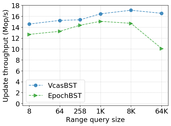
Varying Range Query Size. We show the effect of varying range query size on performance in Figures 2g and 2h (Java), and Figures 2j and 2k (C++). 36 dedicated threads ran range queries and 36 ran updates. Each update thread performs 50% inserts and 50% deletes on a data structure initialized to 100K keys. To better understand the cost of updates and range queries, we plot the throughput of each operation separately.
In Figure 2g, PNB-BST has low update throughput when . This is because their update operations are forced to abort and restart whenever a new range query begins, and thus decreasing range query size lowers update throughput. KST performs decently in most workloads except when each range query covers a significant fraction of the key range, where the update throughput is below 100 operations per second with . This is because their range query performs a double collect of the desired range and is forced to restart if it sees an update in that range.
Data structures that increment a global timestamp with every range query become bottlenecked by this increment when range queries are frequent. This applies to our trees as well as PNB-BST, KiWi, and EpochBST. Consequently, with , LFCA has 3x faster range queries when compared to our trees (Figure 2h). However, LFCA avoids using a global timestamp by having update operations help ongoing range query operations. This helping becomes more frequent and more costly when is large, as shown in Figure 2g. For (about a third of the key range), the update throughput of our trees is 4x faster than LFCA. Other than LFCA, all the other implementations have mostly stable update throughput with varied range size, among which VcasCT-64 has the best overall performance.
Figures 2j and 2k compare the performance of the C++ version of VcasBST with that of EpochBST. Range queries on VcasBST are 4.7–6.3x faster than EpochBST. This is because a range query on EpochBST has to visit three nodes in the retired list for each concurrent delete. Thus, EpochBST visits 1.5–5.5x more nodes in range queries than VcasBST. For updates, VcasBST is at least 7% faster than EpochBST, and up to 64% faster on the largest range query size.
Sorted Workload. In Figure 2i, we test the Java implementations under a sorted workload. We insert an array of sorted keys into an initially empty tree by splitting the array into chunks of size 1024 and placing the chunks on a global work queue; when a thread runs out of work, it grabs a new chunk from the head of the work queue. As expected, the balanced trees, VcasCT-64, KiWi and SnapTree, outperform the unbalanced ones. On 140 threads, SnapTree is 1.4x faster than VcasCT-64, which is in turn 4.1x faster than KiWi.
Overhead of Our Approach. In Figure 2m, we compare our Java implementations VcasBST-64 and VcasCT-64 with the original data structures, BST-64 and CT-64, using 140 threads. The numbers in Figure 2m are normalized to the throughput of BST-64 and CT-64 to make the overheads easier to read. The overall overhead of our approach is low, ranging between 2.7% and 9.1% depending on the workload. This overhead includes the time for epoch-based memory management and the cost of using vCAS and vRead. For VcasBST-64, it also includes the extra actions we take to ensure that deletes satisfy the recorded-once property.
We also measure the overhead of our multi-point queries range, succ, findif, and multisearch, with parameters shown in Figure 3. We compare the throughputs for VcasCT-64 with non-atomic multi-point queries on the original CT-64, which simply run their sequential algorithms (and are not linearizable). Non-atomic multisearch, for example, simply calls find for each key. Figure 3 shows the cost that our approach has to pay to provide query atomicity.
All queries other than succ1 exhibit low overhead: they are between 2.9% and 12.8% slower than their non-atomic counterparts. Having concurrent updates slows down both the atomic and non-atomic queries by about the same amount. For succ1, our scheme exhibits larger overheads (36.8-41.4%) due to the counter bottleneck when the query size is too small.
Summary. Overall, our snapshot approach has low overhead and, despite its generality, performs well compared to existing special-purpose data structures. In particular, VcasCT-64 had the best overall performance in most cases among all the range queryable data structures we evaluated. VcasBST-64 is also competitive on uniform workloads.
References
- (1) Documentation for std::find_if. http://www.cplusplus.com/reference/algorithm/find_if/.
- (2) Java lock-free data structure library. https://bitbucket.org/trbot86/implementations/src/master/java.
- (3) Java weakly consistent iterators. https://docs.oracle.com/javase/8/docs/api/java/util/concurrent/package-summary.html#Weakly.
- (4) Y. Afek, H. Attiya, D. Dolev, E. Gafni, M. Merritt, and N. Shavit. Atomic snapshots of shared memory. J. ACM, 40(4):873–890, Sept. 1993.
- (5) A. Agarwal, Z. Liu, E. Rosenthal, and V. Saraph. Linearizable iterators for concurrent data structures. CoRR, abs/1705.08885, 2017.
- (6) J. H. Anderson. Multi-writer composite registers. Distributed Comput., 7(4):175–195, 1994.
- (7) M. Arbel-Raviv and T. Brown. Harnessing epoch-based reclamation for efficient range queries. In Proc. 23rd ACM Symposium on Principles and Practice of Parallel Programming, pages 14–27, 2018.
- (8) H. Attiya, R. Guerraoui, and E. Ruppert. Partial snapshot objects. In Proc. 20th Symposium on Parallelism in Algorithms and Architectures, pages 336–343, 2008.
- (9) H. Attiya and E. Hillel. Single-version STMs can be multi-version permissive (extended abstract). In Distributed Computing and Networking, 2011.
- (10) H. Avni, N. Shavit, and A. Suissa. Leaplist: Lessons learned in designing TM-supported range queries. In Proc. 2013 ACM Symposium on Principles of Distributed Computing, pages 299–308, 2013.
- (11) D. Basin, E. Bortnikov, A. Braginsky, G. Golan-Gueta, E. Hillel, I. Keidar, and M. Sulamy. KiWi: A key-value map for scalable real-time analytics. In Proc. 22nd ACM Symposium on Principles and Practice of Parallel Programming, pages 357–369, 2017.
- (12) N. Ben-David, G. E. Blelloch, Y. Sun, and Y. Wei. Multiversion concurrency with bounded delay and precise garbage collection. In ACM Symposium on Parallelism in Algorithms and Architectures (SPAA), 2019.
- (13) P. A. Bernstein and N. Goodman. Multiversion concurrency control - theory and algorithms. ACM Trans. Database Syst., 8(4):465–483, Dec. 1983.
- (14) G. E. Blelloch, D. Ferizovic, and Y. Sun. Just join for parallel ordered sets. In ACM Symposium on Parallelism in Algorithms and Architectures (SPAA), pages 253–264. ACM, 2016.
- (15) A. Brodsky and F. E. Fich. Efficient synchronous snapshots. In S. Chaudhuri and S. Kutten, editors, ACM Symposium on Principles of Distributed Computing, pages 70–79, 2004.
- (16) N. G. Bronson, J. Casper, H. Chafi, and K. Olukotun. A practical concurrent binary search tree. In Proc. 15th ACM Symposium on Principles and Practice of Parallel Programming, pages 257–268, 2010.
- (17) T. Brown and H. Avni. Range queries in non-blocking -ary search trees. In Proc. 16th International Conference on Principles of Distributed Systems, volume 7702 of LNCS, pages 31–45, 2012.
- (18) T. Brown, F. Ellen, and E. Ruppert. A general technique for non-blocking trees. In ACM Symposium on Principles and Practice of Parallel Programming (PPOPP), pages 329–342, 2014.
- (19) J. Cachopo and A. Rito-Silva. Versioned boxes as the basis for memory transactions. Science of Computer Programming, 63(2):172–185, 2006.
- (20) B. Chatterjee. Lock-free linearizable 1-dimensional range queries. In Proc. 18th Intl Conf. on Dist. Computing and Networking, pages 9:1–9:10, 2017.
- (21) C. Diaconu, C. Freedman, E. Ismert, P.-A. Larson, P. Mittal, R. Stonecipher, N. Verma, and M. Zwilling. Hekaton: SQL server’s memory-optimized oltp engine. In ACM SIGMOD International Conference on Management of Data (SIGMOD), pages 1243–1254, 2013.
- (22) T. Dickerson. Adapting persistent data structures for concurrency and speculation, 2020.
- (23) J. R. Driscoll, N. Sarnak, D. D. Sleator, and R. E. Tarjan. Making data structures persistent. J. Computer and System Sciences, 38(1):86–124, 1989.
- (24) J. R. Driscoll, D. D. K. Sleator, and R. E. Tarjan. Fully persistent lists with catenation. In ACM-SIAM Symp. on Disc. Algorithms, pages 89–99, 1991.
- (25) F. Ellen, P. Fatourou, and E. Ruppert. Time lower bounds for implementations of multi-writer snapshots. J. ACM, 54(6):30, 2007.
- (26) F. Ellen, P. Fatourou, E. Ruppert, and F. van Breugel. Non-blocking binary search trees. In ACM Symp. on Principles of Distributed Computing, 2010. See also Technical Report CSE-2010-04, EECS Department, York University, 2010.
- (27) P. Fatourou, F. E. Fich, and E. Ruppert. Time-space tradeoffs for implementations of snapshots. In J. M. Kleinberg, editor, ACM Symposium on Theory of Computing (STOC), pages 169–178. ACM, 2006.
- (28) P. Fatourou and N. D. Kallimanis. Time-optimal, space-efficient single-scanner snapshots & multi-scanner snapshots using cas. In ACM Symposium on Principles of Distributed Computing, page 33–42, 2007.
- (29) P. Fatourou, Y. Nikolakopoulos, and M. Papatriantafilou. Linearizable wait-free iteration operations in shared double-ended queues. Parallel Processing Letters, 27(2):1–17, 2017.
- (30) P. Fatourou, E. Papavasileiou, and E. Ruppert. Persistent non-blocking binary search trees supporting wait-free range queries. In Proc. 31st ACM Symposium on Parallelism in Algorithms and Architectures, pages 275–286, 2019.
- (31) S. M. Fernandes and J. Cachopo. Lock-free and scalable multi-version software transactional memory. In ACM Symposium on Principles and Practice of Parallel Programming (PPOPP), page 179–188, 2011.
- (32) F. E. Fich. How hard is it to take a snapshot? In Proc. 31st Conference on Current Trends in Theory and Practice of Computer Science (SOFSEM), volume 3381 of LNCS, pages 28–37, 2005.
- (33) K. Fraser. Practical lock-freedom. Technical report, University of Cambridge, Computer Laboratory, 2004.
- (34) W. Golab, L. Higham, and P. Woelfel. Linearizable implementations do not suffice for randomized distributed computation. In ACM Symposium on Theory of Computing (STOC), 2011.
- (35) T. L. Harris. A pragmatic implementation of non-blocking linked-lists. In International Symposium on Distributed Computing, pages 300–314, 2001.
- (36) M. P. Herlihy and J. M. Wing. Linearizability: A correctness condition for concurrent objects. ACM Transactions on Programming Languages and Systems (TOPLAS), 12(3):463–492, 1990.
- (37) D. Imbs and M. Raynal. Help when needed, but no more: efficient read/write partial snapshot. Journal of Parallel and Distributed Computing, 72(1):1–12, 2012.
- (38) P. Jayanti. -arrays: Implementation and applications. In Proc. 21st Symposium on Principles of Distributed Computing, pages 270–279, 2002.
- (39) P. Jayanti. An optimal multi-writer snapshot algorithm. In ACM Symposium on Theory of Computing (STOC), page 723–732, 2005.
- (40) N. D. Kallimanis and E. Kanellou. Wait-free concurrent graph objects with dynamic traversals. In Proc. 19th International Conference on Principles of Distributed Systems, Leibniz International Proceedings in Informatics, 2015.
- (41) P. Kumar, S. Peri, and K. Vidyasankar. A timestamp based multi-version STM algorithm. In Intl Conf. on Dist. Computing and Networking, 2014.
- (42) M. M. Michael and M. L. Scott. Simple, fast, and practical non-blocking and blocking concurrent queue algorithms. In ACM Symposium on Principles of Distributed Computing, 1996.
- (43) A. Natarajan and N. Mittal. Fast concurrent lock-free binary search trees. In ACM Symposium on Principles and Practice of Parallel Programming (PPOPP), pages 317–328, 2014.
- (44) T. Neumann, T. Mühlbauer, and A. Kemper. Fast serializable multi-version concurrency control for main-memory database systems. In ACM SIGMOD International Conference on Management of Data (SIGMOD), pages 677–689. ACM, 2015.
- (45) Y. Nikolakopoulos, A. Gidenstam, M. Papatriantafilou, and P. Tsigas. A consistency framework for iteration operations in concurrent data structures. In Proc. IEEE International Parallel and Distributed Processing Symposium, pages 239–248, 2015.
- (46) Y. Nikolakopoulos, A. Gidenstam, M. Papatriantafilou, and P. Tsigas. Of concurrent data structures and iterations. In Algorithms, Probability, Networks and Games: Scientific Papers and Essays Dedicated to Paul G. Spirakis on the Occassion of his 60th Birthday, pages 358–369. Springer, 2015.
- (47) C. H. Papadimitriou and P. C. Kanellakis. On concurrency control by multiple versions. ACM Transactions on Database Systems, 9(1):89–99, 1984.
- (48) D. Perelman, R. Fan, and I. Keidar. On maintaining multiple versions in STM. In ACM Symp. on Principles of Dist. Computing, pages 16–25, 2010.
- (49) E. Petrank and S. Timnat. Lock-free data-structure iterators. In Proc. 27th Intl Symposium on Distributed Computing, pages 224–238, 2013.
- (50) D. R. K. Ports and K. Grittner. Serializable snapshot isolation in PostgreSQL. Proc. of the VLDB Endowment, 5(12):1850–1861, Aug. 2012.
- (51) A. Prokopec. Snapqueue: lock-free queue with constant time snapshots. In Proceedings of the 6th ACM SIGPLAN Symposium on Scala, pages 1–12, 2015.
- (52) A. Prokopec, N. G. Bronson, P. Bagwell, and M. Odersky. Concurrent tries with efficient non-blocking snapshots. In Proc. 17th ACM Symposium on Principles and Practice of Parallel Programming, pages 151–160, 2012.
- (53) D. Reed. Naming and synchronization in a decentralized computer system. Technical Report LCS/TR-205, EECS Dept., MIT, Sept. 78.
- (54) T. Riegel, P. Felber, and C. Fetzer. A lazy snapshot algorithm with eager validation. In International Symposium on Distributed Computing, pages 284–298. Springer, 2006.
- (55) N. Sarnak and R. E. Tarjan. Planar point location using persistent search trees. Commun. ACM, 29(7):669–679, 1986.
- (56) Y. Sun, G. E. Blelloch, W. S. Lim, and A. Pavlo. On supporting efficient snapshot isolation for hybrid workloads with multi-versioned indexes. Proceedings of the VLDB Endowment, 13(2):211–225, 2019.
- (57) Y. Sun, D. Ferizovic, and G. E. Blelloch. PAM: parallel augmented maps. In ACM Symposium on Principles and Practice of Parallel Programming (PPOPP), 2018.
- (58) K. Winblad, K. Sagonas, and B. Jonsson. Lock-free contention adapting search trees. In Proc. 30th Symposium on Parallelism in Algorithms and Architectures, pages 121–132, 2018.
- (59) Y. Wu, J. Arulraj, J. Lin, R. Xian, and A. Pavlo. An empirical evaluation of in-memory multi-version concurrency control. Proceedings of the VLDB Endowment (PVLDB), 10(7), Mar. 2017.
Appendix A Detailed Proof of Correctness of versioned CAS and camera Objects
A.1. Linearization Points
Given a camera object and a versioned CAS object associated with it, in this section, we describe how their operations are linearized, but we defer the detailed proof of Theorem 2 to Appendix A.2.
To state the linearization points, we first introduce some useful terminology. When referring to the variables .VHead and .timestamp, we often abbreviate them to VHead and timestamp. We say that a VNode has a valid timestamp at some configuration if the value of its ts field is not TBD at . Otherwise, the timestamp of the node is called invalid. We use the term version list to refer to the list that results from starting at the VNode pointed to by VHead and following the nextv pointers. The head of the version list is the VNode pointed to by VHead.
The only way to modify the version list is the CAS at Line 46, which swings the VHead pointer to a new VNode whose nextv pointer points to the previous head of the version list. This has the effect of adding the new VNode to the beginning of the version list. Before this can happen, initTS is called to install a valid timestamp in the old head of the version list. This ensures that the only VNode in the version list with an invalid timestamp is the first one. At the time a VNode’s timestamp becomes valid, it is therefore still at the head of the version list.
The correctness of readSnapshot operations depends on ensuring that the timestamp associated with a value is current (i.e., in S.timestamp) at the linearization point of the vCAS that stored the value in . So, we linearize a vCAS that adds a VNode to the version list at the time that the timestamp eventually written into that VNode was read from S.timestamp. This means that there may be a VNode at the head of the version list before the vCAS that created that VNode is linearized. This is why any other operation that finds a VNode with an invalid timestamp at the head of the version list calls initTS to help install a valid timestamp in it before proceeding. This helping mechanism is crucial in the argument that all of the following linearization points are well-defined and within the intervals of their respective operations.
- •
A vCAS operation is linearized depending on how it executes.
- –
- –
- –
Finally, consider a vCAS(oldV, newV) operation that returns false on Line 52. This is the most subtle case. The return on Line 52 is only reached when fails its CAS on Line 46 because some other vCAS operation changed VHead after read it at Line 41. We linearize the vCAS immediately after the linearization point of the vCAS operation that made the first such change. (If several vCAS operations that return on Line 52 are linearized immediately after , they can be ordered arbitrarily.)
- •
- •
A readSnapshot operation that terminates is linearized at its last step.
- •
For takeSnapshot operations, let be the value read from timestamp on line 5. A takeSnapshot operation that terminates is linearized when the value of timestamp changes from to .
A.2. Proof of Correctness
In this section, we prove that Fig. 3.1 is a linearizable implementation of versioned CAS and camera objects. First we argue that it suffices to prove linearizability for histories consisting of a single versioned CAS object and a single camera object. Suppose two versioned CAS objects are associated with different camera objects. Then we can prove linearizability for the two sets of objects independently because they do not access any common variables and do not affect each other in terms of sequential specifications. Suppose two versioned CAS objects and are associated with the same camera object . Let be a history of operations on these three objects. Furthermore, let be the history restricted to only operations from and , and similarly, let be the history restricted to only operations from and . We will define the linearization points of so that they are not affected by operations on or . Therefore, showing that both and are linearizable is sufficient for showing that is linearizable because will be linearized the same way in both and .
Let be a history of a versioned CAS object and a camera object . We assume that and are initialized by their constructors (Line 3 and 15, respectively) before the beginning of . We assume this history satisfies the precondition (described in Definition 1) that whenever readSnapshot() is invoked, there must be a completed takeSnapshot operation that returned . When referring to the variables .VHead and .timestamp, we will often abbreviate them to VHead and timestamp.
We first introduce some useful terminology. We say that a VNode has a valid timestamp at some configuration if the value of its ts field is not TBD at . Otherwise, the timestamp of the node is called invalid. We use the term version list to refer to the list that results from starting at the VNode pointed to by VHead and following the nextv pointers. The head of the version list is the VNode pointed to by VHead.
A modifying vCAS operation is one that performs a successful CAS on line 46. Due to the if statement on line 44, if vCAS(, ) is a modifying vCAS operation, then . Note that modifying vCAS operations can return only on line 48 and any operation that returns on line 48 is a modifying vCAS. A vCAS is successful if it is a modifying vCAS or if it returns true at line 44. Otherwise, it is unsuccessful.
We first show that the only change to a version list is inserting a VNode at the beginning of it.
Lemma 1.
Once a VNode is in the version list, it remains in the version list forever.
Proof.
The only way to change a version list is a successful CAS at line 46, which changes VHead from head to newN. When this happens, , so all VNodes that were in the version list before the CAS are still in the version list after the CAS. ∎
It is easy to check that every time we access some field of an object via a pointer to that object, the pointer is not NULL. VHead always points to a VNode after it is initialized on Line 17 of ’s constructor. It follows that every call to initTS is on a non-null pointer. The precondition of readSnapshot(ts) ensures that ts is a timestamp obtained from after was initialized and is therefore greater than or equal to the timestamp that ’s constructor stored in the initial VNode of the version list. Thus, the readSnapshot will stop traversing the version list when it reaches that initial VNode, ensuring that node is never set to NULL on line 34.
Linearization Points.
Before we can define the linearization points, we need a few simple lemmas that describe when VNodes have valid timestamps. We start with an easy lemma about initTS.
Lemma 2.
The following hold:
- (1)
Before initTS is called on a VNode, VHead has contained a pointer to that VNode.
- (2)
After a complete execution of initTS on some VNode, that VNode’s timestamp is valid.
Proof.
All calls to initTS are done on a pointer that has either been read from VHead or successfully CASed into VHead. Once a timestamp is valid, it can never be modified again, since only a CAS on line 22 modifies the ts variable of any VNode. The CAS on Line 22 can fail only if the ts variable is already a valid timestamp. ∎
Lemma 3.
In every configuration , the only VNode in the version list that can have an invalid timestamp is the head of the version list.
Proof.
No VNode’s nextv pointer changes after the VNode is created, so the only way the version list can change is when VHead is updated. Moreover, no VNode’s timestamp ever changes from valid to invalid. So, we must only show that updates to VHead preserve the claim.
The value of VHead changes only when a successful CAS is executed on Line 46 of an instance of vCAS. Consider any such successful CAS by some process and assume the claim holds in the configuration before the CAS to show that it holds immmediately after the CAS. This CAS changes VHead from head to newN. By the initialization of newN on Line 45, that VNode’s nextv pointer is head. So, we must show that head and all VNodes reachable from head by following nextv pointers have valid timestamps when the CAS occurs. Before executing this CAS, executes initTS(head), so, by Lemma 2(2), that VNode’s timestamp is valid at the time that the CAS is executed. Since the CAS is successful, VHead was equal to head immediately before the CAS, so all nodes reachable from that VNode had valid timestamps, by our assumption. ∎
The next lemma is used to define the linearization point of a modifying vCAS.
Lemma 4.
Proof.
By Lemma 2(1), every call to initTS is on a pointer that has previously been in VHead, so has been in the version list before initTS is called. By Lemma 1, is still in the version list when Line 21 and 22 are executed. By Lemma 3, remains at the head of the version list until its timestamp becomes valid when initTS performs Line 22. ∎
We are now ready to define linearization points. As we define them, we argue that the linearization point of each operation is well-defined and within the interval of the operation.
- •
A vCAS operation is linearized depending on how it executes.
- –
If the vCAS performs a successful CAS on Line 46 that adds a node to the version list, and ’s timestamp eventually becomes valid, then the vCAS is linearized on Line 21 of the initTS method that makes ’s timestamp valid. Lemma 4 implies that the linearization point occurs after the vCAS adds to the version list at Line 46. If the vCAS terminates, it first calls initTS on at line 47, so Lemma 2(2) ensures the vCAS is linearized and that the linearization point comes before the end of that initTS.
- –
Let be the value of VHead at Line 41 of a vCAS operation. If the vCAS operation returns on Line 43 or 44, then it is linearized either at Line 41 if ’s timestamp is valid at that time, or the first step afterwards that makes ’s timestamp valid. Lemma 2(2) ensures this step exists and is within the interval of the vCAS, since initTS is called on at line 42.
- –
Finally, consider a vCAS(oldV, newV) operation that returns false on Line 52. This is the most subtle case. The return on Line 52 is only reached when fails its CAS on Line 46 because some other vCAS operation changed VHead after read it at Line 41. We linearize the vCAS immediately after the vCAS operation that made the first such change. (If several vCAS operations that return on Line 52 are linearized immediately after , they can be ordered arbitrarily.)
To argue that this linearization point is well-defined, we must show that the VNode that added to the version list gets a valid timestamp, so that is assigned a linearization point as described in the first paragraph above. By Lemma 1, is still in the version list when reads VHead at Line 51. If is no longer at the head of the version list, then ’s timestamp must be valid, by Lemma 3. Otherwise, if is still the head of the version list, then ’s timestamp is guaranteed to be valid after calls initTS on (Line 51), by Lemma 2(2). So, in either case, is assigned a linearization point, which is before the timestamp of becomes valid. Thus, (and therefore ) is linearized before the end of . Lemma 4 implies that the linearization point of (and therefore of ) is after adds to the version list, which is after reads VHead. This proves that ’s linearization point is inside the interval of .
- –
- •
For a vRead operation that terminates, let be the VNode read from VHead at Line 37. The vRead is linearized at Line 37 if ’s timestamp is valid at that time, or at the first step afterwards that makes ’s timestamp valid. Lemma 2(2) ensures that this step exists and is during the interval of the vRead, since the vRead calls initTS on at Line 38.
- •
A readSnapshot operation that terminates is linearized at its last step.
- •
For takeSnapshot operations, let be the value read from timestamp on line 5. A takeSnapshot operation that terminates is linearized when the value of timestamp changes from to . We know that this occurs between the execution of Line 5 and 6: either the takeSnapshot operation made this change itself if the CAS at line 6 succeeds, or some other takeSnapshot operation did so, causing the CAS on line 6 to fail.
Note that all operations that terminate are assigned linearization points. In addition, some vCAS operations that do not terminate are assigned linearization points.
Proof that Linearization Points are Consistent with Responses Recall that is the history that we are trying to linearize. In the rest of this section, we prove that each operation returns the same response in as it would if the operations were performed sequentially in the order of their linearization points.
Lemma 5.
Assume VHead points to a node in some configuration . If .ts is valid in then either is the VNode created by the constructor of , or the vCAS that created is linearized before the configuration that immediately precedes .
Proof.
Suppose .ts is valid in but is not the VNode created by the constructor of . Then is created by some vCAS operation that added to the head of the version list. Since .ts is valid in , some step prior to set .ts by executing Line 22. The linearization point of is at the preceding execution of Line 21. Thus, the linearization point precedes the configuration before . ∎
We define the value of the versioned CAS object in configuration to be the value that a versioned CAS object would store if all of the vCAS operations linearized before are done sequentially in linearization order (starting from the initial value of the versioned CAS object). The following crucial lemma describes how the value of the versioned CAS object is represented in our implementation. It also says that the responses returned by all readSnapshot and vCAS operations are consistent with the linearization points we have chosen.
Lemma 6.
In every configuration of after the constructor of the versioned CAS object has completed,
- (1)
if VHead points to the VNode created by the constructor of the versioned CAS object, then VHead->val is the value of the versioned CAS object,
- (2)
if the linearization point of the vCAS that created the first node in the version list is before , then VHead->val is the value of the versioned CAS object, and
- (3)
otherwise, VHead->nextv->val is the value of the versioned CAS object.
Moreover, each vRead and vCAS operation that is linearized at or before returns the same result in as it would return when all operations are performed sequentially in their linearization order.
Proof.
We prove this by induction on the length of the prefix of that leads to . In the configuration immediately after the constructor of the versioned CAS object terminates, VHead->val stores the initial value of the versioned CAS object.
Since nextv and val fields of a VNode do not change after the VNode is created, we must only check that the invariant is preserved by steps that modify VHead or are linearization points of vCAS operations (which may change the value of the versioned CAS object) or vRead operations. We consider each such step in turn and show that, assuming the claim holds for the configuration before , then it also holds for the configuration after .
First, suppose is a successful CAS on VHead at line 46 of a vCAS operation. It changes VHead from head to newN, where . By Lemma 3, head->ts is valid when this CAS occurs, since head becomes the second node in the version list. By our assumption, the value of the versioned CAS object prior to the CAS is head->val. Since this step is not the linearization point of any vCAS operation, the value after the CAS is still head->val. By Lemma 2(1) initTS is only called on a pointer that has been in VHead previously, and newN has never been in VHead before this CAS, we know that newN->ts is TBD. So the invariant holds after the CAS, since .
Now, consider a step that is the linearization point of a modifying vCAS(oldV, newV), which we denote , possibly followed by the linearization points of some other vCAS operations that return false on Line 52. Since is a modifying vCAS, it added a new VNode to the head of the version list in front of node . This happens after checks that on Line 43–44 and sets to point to and sets to newV on Line 45. By Lemma 4, is still the head of the version list when step occurs. So in the configuration before , the value in the versioned CAS object is , by our assumption that the claim holds in . Thus, when occurs in the sequential execution, it returns true and changes the value of the versioned CAS object to newV. Note that in . It remains to check that all other vCAS operations that return false at line 52 and are linearized immediately after should return false in the sequential execution and therefore do not change the value of the versioned CAS object. Consider any such vCAS of the form vCAS(oldV’,newV’). By the definition of the linearization point of , makes the first change to VHead after reads it on Line 41. So, must have read a pointer to on Line 41. Since returns false at Line 52, it must have seen at Line 43. Thus, , so when each of the vCAS operations is executed sequentially in linearization order, it should return false and leave the state of the versioned CAS object equal to newV. The claim for follows.
Finally, consider a step that is the linearization point of one or more vRead operations or vCAS operations that return at Line 43 or 44. Consider any such operation . Let be the node at the head of the version list when reads VHead at Line 37 or 41. Then is either this read or a subsequent execution of Line 22 that makes ’s timestamp valid. Either way, VHead points to in , by Lemma 4. By Lemma 5, either case (1) or (2) of the claim applies to configuration . Either way, the value of the versioned CAS object in is . If is a vRead, then it returns as it should. If is a vCAS that returns false at Line 43, it would do the same in the sequential execution in linearization order because reads the state of the versioned CAS object in from on Line 43 and sees that it does not match its oldV argument. If returns true at Line 44, it would also return true when performed in linearization order because the state of the versioned CAS object in matches both ’s oldV and newV values. In all cases the value of the versioned CAS object does not change as a result of , so it is still in , and the invariant is preserved. ∎
The following observation follows directly from the way modifying vCAS operations are linearized.
Observation 7.
Consider a VNode that was added to the version list by a modifying vCAS . If the timestamp of is valid, then .ts stores the value of S.timestamp at the linearization point of .
The following key lemma asserts that version lists are properly sorted.
Lemma 8.
The modifying vCAS operations are linearized in the order they insert VNodes into the version list.
Proof.
Consider any two consecutive VNodes and in the version list, where is inserted into the list before , and let and be the vCAS operations that inserted and to the list, respectively. Recall that the linearization point of a modifying vCAS is at the read of the timestamp (Line 21) of the initTS call that validates the timestamp on the VNode that this vCAS appended to the version list. In particular, a modifying vCAS is linearized after it inserts its VNode into the list (since initTS cannot be called on a VNode before it is inserted, by Lemma 2(1)), but before its VNode is assigned a valid timestamp on Line 22 of initTS. By Lemma 3, a VNode is assigned a valid timestamp before it is replaced as the head of the version list. That is, must be linearized before ’s timestamp was valid, and ’s timestamp became valid before was added to the list. Furthermore, was linearized after was added to the list. Therefore, is linearized before . ∎
Now, we prove our main theorem which says that our versioned CAS and camera algorithms are linearizable and have the desired time bounds.
Proof (Theorem 2).
We show that the return values of each operation is correct with respect to their linearization points. For vCAS and vRead operations, this follows from Lemma 6.
We prove this for takeSnapshot and readSnapshot simultaneously. Suppose a .takeSnapshot operation returns a timestamp , which is passed into a .readSnapshot operation . We show that returns the value of at the linearization point of . Let be the value of VHead on line 32 of . The timestamp of is valid after line 33 of , and by Lemma 3, the timestamps of all the nodes in the version list starting from are valid. This means that on line 34, node->ts is never TBD. Let be the value of node at the last line of and let be the modifying vCAS operation that appended . We know that is the first node in the version list starting from with timestamp less than or equal to . Since is linearized when .timestamp gets incremented from to , by Observation 7, is linearized before the linearization point of . Since returns the value written by , it suffices to show that no modifying vCAS operation gets linearized between the linearization points of and . By Lemma 8, modifying vCAS operations are linearized in the order they appended VNodes to the version list. Therefore, for all nodes that are older than in the version list, their modifying vCAS operations are linearized before the linearization point of . Next, we show that all nodes in the version list that are newer than are linearized after . From the while loop on line 34, we can see that all nodes that lie between and (including , excluding ) have timestamps are larger than . All nodes in the version list that are newer than also have timestamp larger than because they are appended after line 32 of and S.timestamp is already greater than at this step. Therefore, by Observation 7, all nodes in the version list newer than are linearized after the linearization point of . This means is the last modifying vCAS operation to be linearized before the linearization point of , as required.
The bounds on the step complexity of the operations can be derived trivially by inspection of the pseudocode. ∎
Appendix B Adding Linearizable Queries to Concurrent Data Structures
In this section, we show how to use versioned CAS objects to extend a large class of concurrent data structures that are implemented using reads and CAS primitives to support linearizable wait-free queries. Throughout the section we also use NBBST as an example to show how our approach works. The idea of this construction is to replace CAS objects with their versioned counterparts, and to use this to obtain snapshots of the concurrent data structure. We can then run queries on the obtained snapshot, without worrying about concurrent updates to the data structure.
The techniques in this section are general. For many data structures, they allow translating any read-only operation on a sequential data structure into a linearizable query on the corresponding concurrent data structure. To achieve this generality, the techniques go through multiple layers of abstraction. To make it more concrete, we show examples of how to add specific linearizable queries to the Michael and Scott queue (MS96) and NBBST tree (EFRB10) in Appendix E.
We present this construction in two parts. First, we define the concept of solo linearizable queries. A query operation is an operation that does not modify the shared state (i.e., it is read-only). A solo linearizable query (or solo query) is a query operation that is only guaranteed to be correct if it is run solo. Intuitively, a solo query is one that can run on a “snapshot” of a concurrent data structure, and it never changes the current state of the data structure. They may be invoked while other operations are pending, but once invoked, they need to run to completion without any other process taking steps during their interval. Section B.1 describes how to transform a concurrent data structure that supports solo queries (which we refer to as a solo linearizable data structure) into a fully linearizable one using our versioned CAS objects. However, most concurrent data structures in the literature do not come with solo queries. In Section B.2, we discuss how to add solo query operations to a given linearizable data structure.
Definition 1.
We denote by the set of histories of concurrent data structure in which every operation instance from some set of query operations is run solo.
Definition 2.
A concurrent data structure is linearizable with solo queries if every history is linearizable. A query is called a solo linearizable query on . With clear context of solo queries , we call a solo linearizable data structure.
The running time of a solo query may depend on the concurrent state at which it is run. We denote by the running time (number of steps) of a solo query at concurrent state of the data structure.
B.1. Making Solo Queries Fully Linearizable
We now show how to transform a solo linearizable data structure , implemented with CAS objects, that has a set of solo queries , into a fully linearizable data structure . Let be the operations of that are not in . The transformation uses our versioned CAS objects in place of the regular CAS objects of . It preserves all existing correctness guarantees (e.g., linearizability, strong linearizability, sequential consistency) and progress guarantees (e.g., wait-freedom, lock-freedom) of the operations in . Furthermore, it preserves the running time of operations of up to constant factors. The time complexity of a linearizable query in is bounded by ’s time complexity in , plus a contention term.
Construction 3.
To obtain we replace every CAS object with a versioned CAS object, initialized with the same value. All versioned CAS objects are associated with a single camera object. Each CAS or read by an operation in on a CAS object is replaced by a vCAS or vRead (respectively) on the corresponding versioned CAS object. To perform a solo query operation in , a process first executes takeSnapshot on the camera object, to obtain a handle . Then, for any CAS object in that would have accessed, performs readSnapshot() on the corresponding versioned CAS object. Recall that all operations in are read-only, and thus never perform a CAS.
For this construction to be legal, we must show that the precondition for readSnapshot() holds. Namely, we need to show that readSnapshot() is never called on a versioned CAS object that was created after the handle was produced. Intuitively, this is satisfied since no versioned CAS object that was created after can be reachable in the data structure through version nodes with timestamp or earlier, which are the only version nodes that a query reads. The following claim makes the argument more formal.
Claim 4.
In Construction 3, no versioned CAS object is ever accessed using a readSnapshot() operation where was produced before was created.
Proof.
Consider a query operation that uses handle to run on a data structure as prescribed by Construction 3. We say that a versioned CAS object is new if it was created after was produced, and old otherwise. Assume by contradiction that accesses a new vCAS object . must be reachable from the root of for to access it. Note that by the way is initialized, the root must be an old versioned CAS object. Without loss of generality, assume is the first new object that accesses in its execution. must be pointed to by some old versioned CAS object , through which accessed . Since the only updates to versioned CAS objects are via vCAS operations, must have been updated with a vCAS to point to , thereby creating a new version of . Note that since was created after , this update must have also happened after was produced, and therefore the version of that points to has a timestamp larger than . So, executing readSnapshot() on would not access the version pointing to , but some older version instead. This contradicts the fact that reaches . ∎
Using Construction 3, we can make solo queries linearizable with the bounds specified in the following theorem.
Theorem 5.
Given a concurrent data structure with a set of linearizable operations and a set of solo query operations . Construction 3 produces a linearizable data structure that supports operations from both and . This construction maintains the following properties:
- •
Operations from have the same progress properties in as in , and their runtimes are increased by only a constant factor.
- •
Each operation costs where is the concurrent state at which executes the takeSnapshot operation, is the number of vCAS operations concurrent with on memory locations accessed by in the execution, and is the maximum number of repeated accesses to the same object by the query.
The proof is in Appendix C. We note that in most cases, the number of accesses that a query executes to the same object is 1 (or a small constant). If not, this bound can be improved by caching the values read from the data structure locally to avoid the extra overhead of reading it repeatedly from the concurrent data structure.
B.2. Adding Solo Queries to Linearizable Data Structures
Concurrent data structures in the literature are usually designed to support a set of operations that are all linearizable. Thus, the question of whether solo linearizable operations can be easily incorporated is generally not considered when designing these data structures. Is it always possible to run queries in a linearizable manner on a snapshot of any given data structure? How efficient can such queries be? In this section, we address these questions.
While designing queries to run solo is certainly much simpler than designing them to be linearizable in the concurrent setting, it is still not as easy as designing queries for a sequential data structure. This is because, in some cases, linearization points cannot be uniquely determined from the state of shared memory; instead, the linearization points may only be determined at the end of the execution, since they can depend on future events. If this is the case, a query that is run solo cannot determine whether a pending update operation has linearized or not, and, since the query may not change the state, it cannot enforce a placement of the linearization point. Herlihy and Wing (herlihy1990linearizability) describe a queue implementation in which the linearization order of the enqueue operations depends on future dequeue operations. For that algorithm, no solo query is possible. Herlihy and Wing (herlihy1990linearizability) point out that the difficulty in this scenario is the absence of an abstraction function from states of the implementation to states of the abstract data type being implemented. We therefore define the notion of direct linearizability, which intuitively means that there is always such a mapping from every concurrent state in an execution of the concurrent data structure to the abstract state of the abstract data type being implemented.
Definition 6.
An abstraction function of a solo linearizable data structure with solo queries that implements an abstract data type , is a function from concurrent states of to abstract states of such that for every history , there exists a linearization of such that:
- (1)
maps the initial state of to the initial state of (i.e., ).
- (2)
If a concurrent state of , can be obtained from another concurrent state in without the linearization of any operation between and , then they map to the same abstract state (i.e., ).
- (3)
If a concurrent state of , can be obtained from another concurrent state in where operations, , linearized between and in this order, then is the state of that is obtained from applying in this order to .
Intuitively, the abstraction function respects the linearization points in the execution of . At first glance, it seems like the abstraction function’s behavior is determined solely by the update operations from . However, query operations do have an indirect impact because they can affect the linearization points of the update operations, which affects the behavior of the abstraction function. When the definition is applied to fully linearizable data structures, , so is the set of all histories of .
Definition 7.
A linearizable data structure is said to be directly linearizable if it has an abstraction function.
Direct linearizability is reminiscent of strong linearizability (GHW11). Strong linearizability requires that the linearizations can be chosen for histories in a prefix-preserving way: for a prefix of a history , the linearization of must be a prefix of the linearization of . Thus, future events cannot determine whether a given step in the execution was a linearization point or not. Intuitively, direct linearizability requires that update operations be strongly linearizable, but does not require the same behavior from query operations (that do not change the high-level state). Furthermore, while strong linearizability only requires this “prefix preserving” behavior for parts of the state that can be observed by operations of the data structure, direct linearizability imposes this behavior on the entire shared state, regardless of the interface through which operations of the data structure can access it. Appendix D shows that strong and direct linearizability are incomparable. However, all strongly linearizable data structures that we are aware of are also directly linearizable.
Consider the NBBST binary search tree (EFRB10) outlined in Section 4. Recall that NBBST implements the ordered set abstract data type, with keys as elements. To avoid special cases, the tree includes two leaves containing dummy keys.
Proposition 8.
Consider the function that maps concurrent states of the NBBST BST to states of the ordered set abstract data type as follows. Given a concurrent state of NBBST, is the set of keys in leaf nodes reachable from the root in except for the two dummy keys. is an abstraction function of NBBST.
Proof.
This theorem is proved as Lemmas 29 and 30 in the technical report (EFRB10), so we just sketch it here. Initially, the tree has only the two leaves containing the dummy keys, which maps to the empty set, as desired. Each Insert() that modifies the tree is linearized at the child CAS that adds a leaf containing to the tree (and it is shown that was not present in the tree before this change). Similarly, each Delete() that modifies the tree is linearized at the child CAS that removes a leaf containing from the tree. Each Insert() that returns false is linearized when is in a leaf of the tree, and each Delete() that returns false is linearized when there is no leaf containing , so these operations have no effect on the tree or on the abstract state of the set. Each terminating Find() returns true if and only if appears in some leaf at the linearization point of the Find. It follows that each operation is linearized so that its effect on the set of keys stored in leaves exactly matches its effect on the abstract state of the ordered set that the tree implements. ∎
Abstraction functions can help us both design solo queries and prove their correctness. It is often helpful to reason about solo queries based on how they behave on each concurrent state. For this purpose, we present the following definition.
Definition 9.
Let be an operation from a concurrent data structure and let be a reachable concurrent state, we define to be the response value of when run solo on concurrent state .
Now we present a proof technique for showing that a read-only operation is a solo query. Consider a concurrent data structure that implements an abstract data type and is linearizable with solo queries . Suppose has an abstraction function . We add a query operation to to get the ADT and we add to to get . Our goal is to show that is an implementation of that is linearizable with solo queries . The following observation says that it suffices to show for all reachable concurrent states .
Observation 10.
If for any reachable concurrent state , then is an implementation of that is linearizable with solo queries . Furthermore, in this case, is still an abstraction function for .
Note that the set of reachable concurrent states for does not change when we add a read-only operation to . The fact that is still an abstraction function for is important because it allows us add solo queries one at a time. This is summarized by the following observation.
Observation 11.
Suppose two data structures have the exact same linearizable operations , but different solo queries and . If the same abstraction function works for both queries, then adding to the first data structure results in a new data structure that is linearizable with solo queries .
Next, we show how to use the abstraction function as a guide for designing solo queries. If the abstraction function is computable and there is some way of viewing/traversing the state of shared memory, then an easy, but not necessarily efficient, method would be to first traverse the state of , then use the abstraction function to arrive at an abstract state, and finally compute the query on the abstract state. This query literally computes , so we can apply Observation 10. This is inefficient, since traversing the entire concurrent state often takes much longer than executing the query. We show examples of how to compute queries designed for a sequential version of the data structure on a concurrent state.
B.2.1. Solo queries for NBBST
Consider the NBBST. The concurrent state of the NBBST includes a lot of information used to coordinate concurrent updates. By removing everything except the root pointer, the key, left, right fields of each Internal node, and the key fields of each Leaf node, we end up with a standard leaf-oriented BST (with child pointers, but no parent pointers). This means that sequential read-only queries that work on a leaf-oriented BST, such as predecessor or range queries, can be run on the NBBST as is, because they only access fields that we keep. In the following theorem, we show that these read-only queries can be added to the NBBST as solo queries without any modification.
Theorem 12.
Let be a set of read-only, sequential operations on a leaf-oriented BST implementing a set of abstract queries . Let be an ADT that supports ordered set operations as well as queries from . Adding the operations in , without modification, to the NBBST yields a concurrent implementation of that is linearizable with solo queries .
Proof.
Let be the abstraction function from Proposition 8 for NBBST. Pick any and let be the abstract operation that it implements. Our goal is to show that for all reachable concurrent states . Then we can apply Observations 10 and 11 to complete the proof.
We begin by defining a mapping from states of leaf-oriented BSTs to states of and a mapping from concurrent states to states of a leaf-oriented BST. (The in stands for intermediate state because it is in between the abstract state and the concurrent state.) For we use the textbook mapping which maps an leaf-oriented BST to the set of keys that appear in its leaves. Given an leaf-oriented BST state , return value of on state (denoted ) equals . To compute the mapping , we start with a concurrent state and remove everything except the root pointer, the key, left, right fields of each Internal node, and the key fields of each Leaf node. Since only accesses the fields that we keep, it cannot tell the difference between running on a concurrent state and running on . Therefore . It is easy to verify that and this completes the proof because . ∎
We apply Construction 3 on top of Theorem 12 to get a data structure that supports insert, delete, and find, as well as linearizable implementations of any query for which there is a read-only sequential algorithm. By Theorem 5, we maintain the efficiency of insert, delete, and find up to constant factors and for each new query operations in , it is wait-free and its runtime is proportional to the sequential cost of the query plus , where is the number of vCAS operations that occur during the query and that operate on objects accessed by the query, and is the maximum number of repeated accesses to the same object by the query. Most read-only, sequential operations on a leaf-oriented BST, such as predecessor and range_query, can be written so that each query accesses a memory location no more than a constant number of times. For such operations, the added cost is just . For example, consider a range_query operation that computes the list of keys within a certain range. If we start with a sequential implementation that takes time, where is the height of the BST and is the number of keys within the specified range, then the corresponding concurrent query in would take time, where is the height of the concurrent tree at the linearization point of the operation.
The NBBST is an easy example because the function from the proof of Theorem 12 is essentially an identity function. We show a more complicated example with Harris’s linked list in Appendix F. With an appropriately defined , the proof structure we used for Thereom 12 works for Michael and Scott’s queue (MS96), Harris’s linked list (Harris01), Natarajan and Mittal’s BST (NM14), and chromatic BSTs (BER14). For these algorithms, we need to slightly modify the sequential, read-only operations to make them solo queries. The mapping is always defined to be the standard mapping from sequential to abstract state and the key property to prove is that .
Appendix C Proof of Theorem 5
Proof.
We construct from as described by Construction 3. We want to show that is a linearizable implementation of the data structure with all of its operations in and . We do so by mapping each history of to a history of in which all solo linearizable queries are run in isolation, and in which all read and CAS operations return the same values as the readSnapshot, vRead and vCAS operations in . Furthermore, and will have the exact same high-level history.
Given a history of , we map it to a history of as follows. (1) For every query operation we move all readSnapshot() operations executed by to appear immediately after the takeSnapshot that returned , in the same order. We then remove the takeSnapshot, and replace all readSnapshot() operations with reads of the corresponding CAS objects of . (2) For every vRead or vCAS operation that appears in , we simply map it to a read or CAS (respectively) on the corresponding CAS object in , without moving it in the history.
Note that by the definition of the versioned CAS object, vRead and vCAS behave the same as read and CAS in CAS objects. Furthermore, note that the only operations that are moved in to form are readSnapshot operations, which do not affect the state of the versioned CAS object they operate on. Thus, all read and CAS operations in return the same values that their corresponding vRead and vCAS operations returned in . Recall from the definition of the versioned CAS object that readSnapshot() always returns the value of the versioned CAS object it operates on at the time that handle was produced. Thus, a read of a CAS object in executed at the concurrent state at which the handle was produced returns the same value as the readSnapshot() operation anywhere in the history .
Since is a solo linearizable data structure and is a legal history of in which all solo operations run in isolation, is a linearizable history. Since all operations in return the same values as they return in , is also linearizable. Furthermore, we can linearize any operation in at the same step as it linearizes in (where we map steps of to steps of in the same way as above), and any operation at its takeSnapshot operation.
To show the required running time bounds, note that operations in and operations in access the same number of base objects. The difference in running time for operations in is strictly due to the time it takes to access the versioned CAS object for vCAS and vRead operations. By Theorem 2, this amounts to constant overhead. Operations execute one takeSnapshot operation, which takes constant time, and then replace every read they would do in the implementation of with a readSnapshot() where is the handle returned by the takeSnapshot. By Theorem 2, the running time of each readSnapshot() is proportional to the number of successful vCAS operations on that object since was produced. Note that all such vCAS operations on all versioned CAS objects that the query accesses are concurrent with the query itself. Thus, we get our desired time bounds. ∎
Appendix D Relationship of Strong Linearizability to Direct Linearizability
Strong linearizability was introduced by Golab, Higham and Woelfel (GHW11) to provide a stronger guarantee that permits reasoning about concurrent executions that involve randomness. At first glance, it seems that this condition might be what is required for our approach to be applicable. We show here that strong linearizability is not comparable to direct linearizability (defined in Definition 7), which is the property required for our approach.
Intuitively, an implementation is strongly linearizable if linearization points for each operation can be chosen as the execution proceeds, without needing to know what happens later in the execution. (See (GHW11) for the formal definition; the informal definition will suffice for this discussion.)
We first show that strong linearizability does not imply direct linearizability. Consider a non-deterministic ADT stores a single bit and provides the following two operations. Write-random-bit, which sets the bit to either 0 or 1, non-deterministically, and returns ack). Read simply returns the current value of the bit. Let be an implementation that delays the choice of the random bit written by a write-random-bit until the first subsequent read operation. More precisely, uses a writable CAS object with three possible states, . A write-random-bit operation simply writes into . A read does a CAS() and returns the new value if the CAS is successful, or the old value if the CAS is unsuccessful. Since each operation performs only one shared-memory access in , that access must serve as the linearization point of the operation. It is easy to see that this linearization is correct. Thus, linearization points can be determined without having to know what happens later in the execution. In other words, is strongly linearizable. However, is not directly linearizable: when is in state , there is no abstract state that can be used as the value of the abstraction function . If , then an execution in which the subsequent read returns 1 would violate Definition 6. A similar problem arises if .
Indeed, our approach would fail if we tried to apply it to : if a takeSnapshot is performed between a write-random-bit and the first subsequent read, reading the snapshot would yield , and it would be impossible to conclude what state of this corresponds to. Thus, strong linearizability is not a sufficient condition for our approach to be applicable.
Next, we show that direct linearizability does not imply strong linearizability. The snapshot ADT (AADGMS93) stores a vector of values and allows processes to update components of the vector or perform a scan that reads the whole vector atomically. The classic implementation of (AADGMS93) implements a snapshot using an array of values (with associated timestamps to avoid ABA problems). Updates are performed by writing the new value to the appropriate location in the array and changing its timestamp. A scan reads the array repeatedly until getting identical results twice. This implementation is not strongly linearizable (GHW11), but it is directly linearizable: the abstraction function simply strips the timestamps from the elements stored in the array to get the state of the ADT.
Appendix E Examples
Our first example focuses on the concurrent queue implementation by Michael and Scott presented in (MS96). We will call this implementation MS-Queue. Thus, we have , and is the abstract data type of a FIFO queue that stores integers and supports the operations enqueue and dequeue.
We start by describing how MS-Queue works. MS-Queue (MS96) implements the queue using a simply-linked list of Node objects, each storing a key and a next pointer pointing to the next Node. Two pointers, called Head and Tail, point to the first and the last element of the list that implements the queue, respectively. The first Node of the list is always a dummy Node. Thus, the elements of the queue are the keys of the Nodes starting from the second Node of the list up until its last Node. Initially, the list contains just the dummy Node, whose key can be arbitrary and its next pointer is equal to NULL. At each point in time, the list contains those elements that have been inserted in the queue and have not yet been deleted, in the order of insertion. It also contains the last element that has been dequeued as the first element of the list (i.e., as the dummy Node).
To insert a key in the queue, a process has to call Enqueue(). Enqueue first allocates a new Node with key and its next field equal to NULL. It then reads Tail and checks whether the next field of the Node it points to is equal to NULL. If this is so, Tail points to the last element of the queue, and Enqueue attempts to insert after this Node using a CAS. If this CAS is successful, then performs one more CAS trying to update Tail to point to . Otherwise, some other process managed to insert its own Node as the next to the last one, so has to retry. If the Node pointed to by Tail does not have its next field equal to NULL, then some process has managed to insert its own Node as the next Node to the one pointed to by Tail but it has not yet updated Tail to point to this Node (i.e., Tail is falling behind). To ensure lock-freedom, whenever discovers that Tail is falling behind, it helps by updating Tail to point to the last Node of the list, before it restarts its own operation.
A process executing Dequeue, reads both Head and Tail. If they both point to the same Node and the next field of this Node is NULL, then the queue is empty (it contains just the dummy Node) so false is returned. If they point to the same Node, but the next field of this Node is not NULL, then Tail is falling behind, so has to help by performing a CAS to update Tail to point to the last Node of the queue before it retries its own operation. If Head and Tail do not point to the same Node, Dequeue reads the key of the second Node of the list and performs a CAS in an effort to update Head to point to this Node. If the CAS is successful, Dequeue completes by returning the key that it read (and the Node from where it read this key becomes the dummy Node). Otherwise, restarts the execution of Dequeue.
In MS-Queue, the Head pointer always points to the first element of the list, whereas the Tail pointer always points either to the last or to the second last pointer of the list. This implies that whenever the next pointer of the last element of the list changes to point to a newly inserted Node, Tail points to the last Node of the list. Moreover, whenever Head is updated, Tail does not point to the first element of the list. These properties and the way helping is performed make it possible to assign linearization points to the queue operations in two different ways. A Dequeue is linearized when Head is updated to point to the list Node whose element the Dequeue returns. An Enqueue can be linearized either at the point the next field of the last Node changes to point to the newly inserted Node, or it can be linearized when the Tail pointer changes to point to the newly inserted Node (notice that the latter change might not be performed by the same process that initiated the Enqueue). Note that whenever Dequeue interferes with Enqueue, i.e., whenever there is just one element in the queue, Dequeue first updates Tail to point to the last Node (if needed) and then performs the deletion. In this way, Head is never ahead of Tail and therefore the linearization point of an Enqueue always precedes the linearization point of the Dequeue that deletes the element that the Enqueue inserted in the list. (Note that this is true for both ways of assigning linearization points.) It is also not hard to prove that the list is always connected, and the Nodes are appended at the end of the list, and that they are extracted from the beginning of it, in the order defined by the sequence of the linearization points assigned to Enqueue operations.
Note that the way we choose to assign linearization points allows us to determine the annotations for the executions of MS-Queue (in a straightforward way). Note that both linearization schemes, assign the linearization point of an operation at the point in time that a concrete CAS is executed, i.e. each linearization point is assigned at the point that an internal actions of the MS-Queue I/O automaton occurs. This allows us to come up with an abstraction function in each case.
Figures E and E show how to implement two kinds of read-only queries on top of MS-Queue using versioned CAS objects. The first, called peekEndPoints, returns the values of the first and the last element in the queue. The second implements scan, i.e., it returns a set containing the keys of all queue Nodes.
To implement these queries, we have to perform the simple changes to MS-Queue described in Section 4. We call the resulting algorithm Ver-Queue. In Ver-Queue, Head and Tail are versioned CAS objects storing references to VNode objects whose val field points to the first and the last Node of the list, respectively. Similarly, the next field of each Node is a versioned CAS object storing a reference to a VNode object that contains the pointer to the next Node in the queue. The code for Enqueue and Dequeue remains unchanged but every read to Head, Tail or to the next field of a Node has to be replaced with an invocation of vRead (on the same object). Similarly, every CAS on each of these objects, has to be replaced with a vCAS (on the same object with the same old and new values). We remark that all versioned CAS objects are associated with a single camera object . A takeSnapshot is invoked on this camera object at the beginning of every query.
PeekEndPoints starts by performing a takeSnapshot and storing the resulting handle into a local variable ts. Finally, it executes readSnapshot(ts) to read both Head and Tail and returns the values it read.
A scan first executes takeSnapshot to get a handle ts, and also reads Head and Tail using readSnapshot(ts). Then, it executes a while loop to traverse the list starting from the node pointed to by the value read in Head until the node pointed to by the value read in Tail. It uses a set to collect the pointers of the nodes it traverses (other than the first one) and returns this set at the end. On each node, it calls readSnapshot(ts) to move to the next node. This ensures that updates that occured in the list after the point that the global timestamp was increased will not be included in the set.
E.1. A Versioned Concurrent BST Implementation based on the NBBST
We start with a brief, informal description of the concurrent binary search tree (BST) implementation provided in (EFRB10), which we will call NBBST. NBBST implements a leaf-oriented tree, i.e., a tree that represents a set whose elements are the keys stored only in the leaf nodes of the tree. The tree is full, i.e., every internal node has exactly two children. Moreover, the tree satisfies the following sorting property: for every internal node with key , the key of every node in the left subtree of is smaller than , whereas every node in the right subtree of has key larger than or equal to .
NBBST supports three operations, Insert(), Delete(), and Find(), where is a key. All three operations start by calling Search(), a routine that searches for by following the standard BST searching algorithm. Search returns a pointer to the leaf that it arrives, a pointer to its parent node, and a pointer to the grandparent of this leaf. Find simply checks whether the leaf node returned by Search contains key . If it does, it returns true, otherwise false is returned.
In its sequential version, Insert replaces the leaf that the Search arrives at with a BST of three nodes, two leaves containing the key of the node pointed to by and the newly-inserted key, and an internal node containing the larger key among the keys of the two leaves. The replacement is performed by switching the appropriate pointer of from to the root of this BST. Delete essentially performs the inverse action: it switches the appropriate child pointer of from to the sibling of the node pointed to by , thus replacing a part of the tree that is comprised of three nodes (one of which is the leaf to be deleted) with one node, namely the sibling of the node to be deleted.
To avoid synchronization problems, NBBST uses CAS to apply a change to a child pointer of a node. Such a CAS is called a child CAS. Morover, it flags a node when its child pointer is to be changed, and unflags it after the change of the child pointer has been performed. These two types of CAS are called flag CAS, and unflag CAS, respectively. Thus, NBBST uses flagging to “lock” a node (in a non-blocking manner) whose child pointer is to be changed. NBBST marks an internal node when the node is to be deleted. It does so by executing a mark CAS. A marked node remains marked forever. To implement flagging and marking, each node has a two-bit status field, which can have one of the following four values: Clean, Flag for insertion, Flag for deletion, or Mark. A flag or mark CAS can succeed only if it is applied on a node whose status is Clean. If a flag CAS fails, the process that performed the flag CAS retries the execution of its operation by starting it from scratch. If the operation is a Delete and the flag CAS succeeds but the mark CAS fails, then the process first unflags , using a backoff CAS, and then retries the execution of its operation.
To ensure lock-freedom, each process executing an operation records in an Info object all the information needed by other processes to complete the operation. A pointer to such an object is stored together with the status field of a node (and they are manipulated atomically). A process that fails to flag or mark a node helps the operation that has already flagged or marked the node to complete (by reading the necessary information in the Info object pointed to by the status field of the node). Then, restarts its own operation. This ensures that a single operation cannot repeatedly block another operation from making progress. Thus, lock-freedom is ensured.
For NBBST, it is proved that each node a Search() visits was in the tree, on the search path for , at some time during the Search. Search() is linearized at the point when the leaf it returns was on the search path for . The insert and delete operations that return false are linearized at the same point as the Search they perform. Every insert or delete operation that returns true has a unique successful child CAS and the operation is linearized at that child CAS.
Figures E.1 and E.1 show how we can modify NBBST to support queries using versioned CAS objects. We call the resulting algorithm Ver-BST. They also provide pseudocode for RangeSum(), a query that returns the set of those keys in the implemented set that are larger than or equal to and smaller than or equal to .
In Ver-BST, the child[LEFT] or child[RIGHT] field of each internal Node is a versioned CAS object storing a reference to a VNode object that contains the pointer to the left or right child, respectively, of in the tree. Moreover, every read of the child[LEFT] or child[RIGHT] field of a Node is replaced with an invocation of vRead (on the same object). Similarly, every CAS on each of these fields, is replaced with a vCAS (on the same object with the same old and new values). We remark that the status field of a Node does not have to be a versioned CAS object, as queries simply ignore the flag and mark signs on the Nodes. Notice that all versioned CAS objects are paired with the same camera on which a takeSnapshot is invoked at the beginning of the execution of every query.
RangeSum() first performs a takeSnapshot. Then, it calls the recursive function RSTraverse which traverses part of the tree to perform the required calculation. Pseudocode for RangeSum is provided in Figure E.1.
In Ver-BST, linearization points can be assigned to insert and delete operations the same way as in NBBST. A query is linearized at the linearization point of the takeSnapshot it invokes on Line 2.
Appendix F Solo queries for Harris’s Linked List
Each node in the Harris linked list contains a key field and a next field. The next field stores a pointer that is potentially marked, indicating that the node containing this next field has been logically deleted. A state of the Harris linked list consists of a set of nodes and a pointer to the first node in the linked list.
The technique we use from constructing solo is similar to the technique we applied to the NBBST in Section B.2.1. Just like the NBBST, Harris’s linked list implements an ordered set ADT. First, we define to be the standard mapping from sequential linked lists to ordered sets which basically maps a linked list to the set of keys that appear in its nodes. If is a read-only, sequential linked list operation implementing the abstract query , then by the correctness of , we know that for all sequential states . Just like in Section B.2.1, we use to denote the return value of when run on state . Next, we define a mapping from concurrent states to sequential linked list states such that is an abstraction function. For each sequential, read-only linked list operation implementing the abstract query , we show how to modify into a read-only operation for the Harris linked list such that for all reachable concurrent states , . Once we have these facts, it is fairly straight-forward to complete the proof. From the equalities we’ve proven for all reachable concurrent states , so by Observation 10, can be added to Harris’s linked list as a solo query.
In Harris’s original paper (Harris01), he linearizes successful insert operations when the node being inserted gets connected to the data structure and successful delete operations when the node being deleted gets marked for deletion (i.e. when the node gets logically deleted, not physically deleted). We need to define so that the abstraction function is consistent when these linearization points. To compute , we physically delete (i.e. unlink) all the logically deleted nodes from and return the resulting linked list as the sequential state. Using an argument similar to the proof of Proposition 8, we can show that is an abstraction function for Harris’s linked list.
Now we show how to transform into . Let be a read-only, sequential linked list operation implementing the abstract query . To construct , whenever reads the next pointer of a node, change it to call the getNext function implemented in Figure F. This function basically skips over any marked nodes and returns the next unmarked node. This effectively ignores logically deleted nodes. Therefore, running on a reachable concurrent state has the same effect as running on . Plugging all this into the proof framework we specified earlier shows that can be added to Harris’s linked list as a solo query.
Appendix G Direct versioned CAS Algorithm
Here we consider the correctness and give pseudocode for the optimization that avoid indirection. Consider two versioned CAS objects and . Roughly speaking, since all nodes are recorded-once, every vCAS operation on any versioned CAS object stores a distinct value. This means that every time a vCAS is executed (on any versioned CAS object), it writes a pointer to a newly allocated node. Thus, the only way for a node other than the last in the version list of , to appear in the version list of , is if a pointer to were used as the initial value of . Hence is the last node in ’s version list. We argue that no invocation of OptreadSnapshot on a versioned CAS object traverses the nextv pointer of the last node in the version list of . These imply that the version lists of versioned CAS objects behave as if they are disjoint. In particular, we never have to store nextv pointers for two different version lists in the same node. Based on the above arguments, we can prove that is linearizable. We present pseudo-code for optimized versioned CAS objects in Figure F.