Analysis of a splitting scheme for a class of nonlinear stochastic Schrödinger equations
Abstract.
We analyze the qualitative properties and the order of convergence of a splitting scheme for a class of nonlinear stochastic Schrödinger equations driven by additive noise. The class of nonlinearities of interest includes nonlocal interaction cubic nonlinearities. We show that the numerical solution is symplectic and preserves the expected mass for all times (trace formula). On top of that, for the convergence analysis, some exponential moment bounds for the exact and numerical solutions are proved. This enables us to provide strong orders of convergence as well as orders of convergence in probability and almost surely. Finally, extensive numerical experiments illustrate the performance of the proposed numerical scheme.
AMS Classification (2020). 60-08. 60H15. 60M15. 65C20. 65C30. 65C50. 65J08
Keywords. Stochastic partial differential equations. Stochastic Schrödinger equations. Splitting integrators. Strong convergence. Geometric numerical integration. Trace formulas.
1. Introduction
Deterministic Schrödinger equations are widely used within physics, plasma physics or nonlinear optics, see for instance [79, 2, 23, 64]. In certain physical situations it may be appropriate to incorporate some randomness into the model. One possibility is to add a driving random force and obtain a stochastic partial differential equation (SPDE) of the form
considered for , the -dimensional torus, with periodic boundary conditions. The nonlinearity and the white noise are described in details below. See Equation (1) for the formulation of this problem as a stochastic evolution equation. The stochastic nonlinear Schrödinger equations are used as nonlocal models of wave propagation in several physical applications, see for example [44, 45, 46, 50, 48, 49, 65] and references therein for further details and applications. The nonlinearities we shall consider encompass for instance the cases of an external potential and of a nonlocal interaction cubic nonlinearity . The latter nonlocal interaction function is defined using the convolution of a sufficiently regular interaction kernel with the density function . The stochastic models that we consider have a structure similar to those of the deterministic Schrödinger–Poisson equations or Hartree equations, which are simplified models for fundamental equations in quantum transport where nonlocal interaction terms appear, see for instance [23, 64] and references therein. Such nonlinearities are also used in modeling deterministic problems arising in quantum physics, chemistry, materials sciences, and biology, see for instance [7, 14]. Nonlocal interaction terms for deterministic models can be obtained by mean-field limits starting from many body systems, see for instance [56, 9]. We are not aware of similar derivation for stochastic models. Regarding the numerical treatment of nonlocal interaction terms for Schrödinger equations with white noise dispersion, we refer to the recent article [19].
It is worth mentioning that the error analysis below requires stringent regularity assumptions on the interaction kernel . These conditions are not satisfied, for instance, for the Schrödinger–Poisson case (where ), for the cubic case (where ) or the more general power-law case (where with ). Note that some of the techniques presented below may be used to study numerical schemes for such nonlinearities. This is left for possible future works.
Let us now review the literature on temporal discretizations of stochastic Schrödinger equations, first for equations driven by an Itô noise. In [48], a Crank–Nicolson scheme is studied for the stochastic Schrödinger equation with regular coefficients. First order of strong convergence, resp. rate one half is obtained in the case of additive noise, resp. multiplicative Itô noise. In addition, convergence in probability as well as almost-surely are studied for the case of a power-law nonlinearity. Finally, in the case of smooth and bounded nonlinearity, weak order one is proved in [48]. Observe that the numerical scheme from [48] is implicit. The references [51, 10] present thorough numerical simulations and numerically study the effect of noise in the stochastic Schrödinger equation with a power-law nonlinearity. The work [57] provides a strong convergence analysis of a splitting strategy to the variational solution of a stochastic Schrödinger equation with regular coefficients. The recent article [5] proves strong convergence of an exponential integrator for stochastic Schrödinger equations with regular coefficients. In addition, longtime behaviors of the numerical solutions of a linear model is investigated. The paper [60] provides a convergence rate of the weak error under noise discretizations of some Schrödinger equations. The work [61] shows convergence in probability of a stochastic (implicit) symplectic scheme for stochastic nonlinear Schrödinger equations with quadratic potential and an additive noise. The article [29] proves weak error estimates for a spatial as well as temporal numerical approximation of the stochastic cubic Schrödinger equation with damping and trace-class noise. The recent work [40] proves strong rate as well as weak rate of a splitting scheme when applied to a damped stochastic cubic Schrödinger equation with linear multiplicative trace-class noise and large enough damping term. The very recent preprint [39] provides several convergence results for a structure-preserving splitting strategy when applied to nonlinear stochastic Schrödinger equations with damping term and multiplicative noise. There is a vast literature on the numerical analysis of stochastic nonlinear Schrödinger equations with Stratonovich noise and power-law nonlinearities. Without being exhaustive, we mention the work [47] which proves convergence in probability of the Crank–Nicolson scheme applied to such equations with a spatially correlated noise. The work [70] provides first order of convergence in probability and in the almost-sure sense for a splitting scheme applied to the cubic case. The article [28] shows strong order one of convergence in the local sense of the -scheme when applied to the stochastic cubic Schrödinger equation with a trace-class noise. Strong rate of convergence one for a finite difference approximation of the stochastic cubic Schrödinger equation with a colored noise is shown in [41]. The recent article [42] shows optimal strong order of convergence of a splitting Crank–Nicolson scheme when applied to the spectral Galerkin spatial discretization of the stochastic cubic Schrödinger equation with trace-class noise.
In the present work, we shall analyze a splitting strategy for an efficient time integration of a class of nonlinear stochastic Schrödinger equations, see Equation (1). In a nutshell, the main idea of splitting integrators is to decompose the vector field of the original evolution equation in several parts, such that the arising subsystems are exactly (or easily) integrated. We refer interested readers to [58, 15, 74] for details on splitting schemes for ordinary and partial differential equations. Splitting schemes are also very popular and efficient numerical integrators for stochastic differential equations: we refer the interested reader to the articles [77, 18, 67, 1, 3, 20, 35, 25], the list of references is not exhaustive. For stochastic partial differential equations, splitting schemes have been studied for instance in the following works [72, 38, 57, 69, 11, 52, 8, 42, 78, 21, 22, 12, 73, 19, 24]. The splitting scheme considered in this publication is given by equation (8).
Despite the fact that splitting schemes are widely used for an efficient time integration of deterministic Schrödinger-type equations, see for instance [16, 13, 71, 53, 55, 70, 6], we are not aware of a numerical analysis of such integrators approximating mild solutions of nonlinear stochastic Schrödinger equations driven by an additive noise. In the present work, we intend to fill this gap for a class of nonlinear SPDEs and the main results of this paper are the following:
- •
bounds for the exponential moments of the mass of the exact and numerical solutions (Theorem 11);
- •
a kind of longtime stability, namely a so-called trace formula for the mass, of the exact and numerical solutions (Proposition 6);
- •
preservation of symplecticity for the exact and numerical solutions (Proposition 9);
- •
Observe that, since the nonlinearity in the class of stochastic Schrödinger equation considered here may not be globally Lipschitz, we employ the exponential moments estimates mentioned above to obtain strong rates of convergence, see Propositions 13 and 14. In these propositions, we consider moments of the error multiplied by an exponential discounting factor, and obtain the expected rate of convergence for this quantity. This technique is similar to the approach in [63]. Combining those estimates with the above exponential moment bounds (Theorem 11) to remove the exponential discounting factor, we can then obtain Theorem 15. Note finally, that the choice of a splitting strategy is crucial in obtaining exponential moment bounds for the numerical solution.
Let us mention that in Corollary 17 one obtains orders of convergence and in the sense of convergence in probability and almost sure convergence (depending on a regularity parameter) which are expected to be optimal, whereas in Theorem 15 the orders of convergence in the strong sense may not be optimal. This is due to the exponential moment bounds used in the proofs.
We begin the exposition by introducing some notations, present our main assumptions and provide several moment bound estimates for the exact solution to the considered SPDE. We then present the splitting scheme and study some geometric properties of the exact and numerical solutions in Section 3. The main results of this publication are presented in Section 4. In particular, exponential moments in the norm of the exact and numerical solutions are given, as well as several convergence results. More involved and technical proofs of results needed for convergence estimates are provided in Section 5. Various numerical experiments illustrating the main properties of the splitting scheme when applied to stochastic Schrödinger equations driven by Itô noise are given in Section 6. The paper ends with an appendix containing proofs of auxiliary results.
We use to denote a generic constant, independent of the time-step size of the numerical scheme, which may differ from one place to another.
2. Setting
In this work, we consider the following class of stochastic nonlinear Schrödinger equations
| (1) | ||||
where the unknown is a stochastic process with values in the Hilbert space of square integrable complex-valued functions defined on the -dimensional torus . Details concerning the regularity and growth properties of the nonlinearity and the covariance operator are provided below. In addition, is a real parameter measuring the size of the noise . The initial condition is deterministic, however the results below can be adapted to random initial conditions, satisfying appropriate integrability conditions, using a standard conditioning argument. The space is equipped with the norm , where for all ,
The Sobolev spaces and are Hilbert spaces, and the associated norms are denoted by and . The notation will also be used below. For , let also denote the norm in the Banach space of functions of class defined in .
Solutions of (1) are understood in the mild sense:
| (2) |
where . Let us state the following result (see e.g. [68, Lemma ] and [48, Appendix A.]).
Lemma 1.
The linear operator generates a group of isometries of , such that for all , all , and all , one has
In addition, for , there exists such that for all and all ,
The Wiener process , with covariance operator , in the SPDE (1) is defined by
where is a complete orthonormal system of , is a sequence of independent real-valued standard Wiener processes on a stochastic basis , and is a sequence of complex numbers such that . The linear operators and are defined by and , for all .
For a linear operator from to , and any complete orthonormal system of , we define
This definition is independent of the choice of the orthonormal system.
With this notation, (whenever the sum is finite).
We now set the assumptions on the spatial Sobolev regularity of the noise as well as on the nonlinearity in the stochastic Schrödinger equation (1) required to prove well-posedness for the SPDE (1), to prove -regularity of the solution, and to show strong convergence of order of the proposed splitting integrator in Section 4.
Assumption 1.
One has
The nonlinearity satisfies for all , where is a real-valued mapping. Furthermore, it is assumed that if (i. e. the potential is a function of the modulus).
In addition to the above, assume that the mapping is locally Lipschitz continuous with at most cubic growth: there exists and such that for all , one has
| (3) |
Finally, there exists and a polynomial mapping , such that for all , one has
| (4) | ||||
In the above and in the sequel, denotes the gradient of the mapping .
Note that assuming that is real-valued for all implies that one has the equality .
The value of the real number appearing in the right-hand side of (3) plays a crucial role in the convergence analysis below.
Let us recall the definition of the stochastic integral in the mild form (2) and the associated Itô isometry property. If for all , is a linear operator from to , the stochastic integral is understood as , and the Itô isometry formula is given by
Under Assumption 1, the stochastic convolution is thus well-defined and takes values in . It solves the linear stochastic Schrödinger equation driven by additive noise
Most of the analysis can be performed when Assumption 1 is satisfied, in particular we will prove below that (1) admits a unique global solution, and that the splitting scheme has a convergence order . To get convergence order of the proposed splitting integrator for the semilinear problem (1), we need further assumptions.
Assumption 2.
On top of Assumption (1), let us assume that one has
Furthermore, let us assume that the nonlinearity is twice differentiable, and there exists such that for all , one has
| (5) | ||||
Finally, let us assume that there exists and a polynomial mapping , such that for all , one has
| (6) | ||||
In the above and in the sequel, denotes the Hessian matrix of the mapping .
Next, we verify that the two examples of nonlinearities seen in the introduction, namely and , verify these conditions. First, the conditions in Assumption 1 or 2 are satisfied in the case of a linear mapping , where the external potential function is a real-valued mapping of class , with (resp. ) to satisfy Assumption 1 (resp. Assumption 2). In that case, the mapping is globally Lipschitz continuous, and (3) holds with and . Second, the conditions in Assumption 1 or 2 also hold for the following class of nonlocal interaction cubic nonlinearities. Note that in this case.
Proposition 2.
Let and let be a real-valued mapping of class . For every , set
where denotes the convolution operator.
Proof.
Observe that for any , the mapping is of class , with for . It thus follows that for all .
First, assume that . Let us check that (3) holds. Let , then one has
Thus (3) holds with and . The conditions in (4) follow from straightforward computations.
Second, assume that . The conditions in (5) follow from writing, for all ,
The conditions in (6) follow from straightforward computations.
This concludes the proof of Proposition 2. ∎
Note that the conditions in Assumption 1 or 2 are not satisfied in the standard cubic nonlinear Schrödinger case, where , or for other (non-trivial) power-law nonlinearities, or for the logarithmic nonlinearity considered in the recent preprint [43], or for the stochastic Schrödinger–Poisson equation with a non-smooth potential .
Remark 3.
The result of Proposition 2 remains valid if is an arbitrary smooth bounded domain and homogeneous Dirichlet boundary conditions are imposed, instead of periodic boundary conditions, under appropriate assumptions on the potential .
To conclude this section, let us state a well-posedness result for the stochastic Schrödinger equation (1) in terms of mild solutions (2), and several moment bound estimates. Note that additional bounds for the exponential moments in of the exact solution are given in Section 4.
Proposition 4.
Let Assumption 1 be satisfied.
For any initial condition , there exists a unique mild solution of the stochastic Schrödinger equation (1), which satisfies (2) for all . In addition, for every , , , and , there exists such that one has a moment bound in
with , resp. , when Assumption 1, resp. Assumption 2, is satisfied.
Finally one has the following temporal regularity estimate: for all ,
The proof uses standard arguments and is postponed to the appendix.
3. Splitting scheme
In this section we define a splitting integrator for the stochastic Schrödinger equation (1) and show some geometric properties of this time integrator. The main idea of splitting schemes is to decompose the original problem, equation (1) in our case, into subsystems that can be solved exactly (or efficiently numerically). Splitting schemes are widely used for time discretization of deterministic cubic Schrödinger equations, see, e.g. the key early reference [59].
The definition of the splitting scheme studied in this article relies on the flow associated with the differential equation . For all and , define
| (7) |
Since is real-valued by Assumption 1, one has for all , which gives using Assumption 1 or 2. It is then straightforward to check that is the flow associated with the differential equation . Indeed, for all and all , one has
Observe that the flow of the above ODE preserves the -norm: one has for all and all .
The splitting scheme for the stochastic Schrödinger equation (1) considered in this article is then defined by the explicit recursion
| (8) |
where denotes the time-step size, and are Wiener increments. Recall that is defined after equation (2). Without loss of generality, it is assumed that . The scheme is obtained using a splitting strategy: at each time step, first one may write , i. e. the equation with initial condition is solved exactly, second one has , which comes from applying an exponential Euler scheme to the stochastic differential equation . Observe that bounds for the exponential moments in of the numerical solution are given in Section 4.
Remark 5.
Alternatively, solving exactly the stochastic differential equation yields the following numerical scheme for the SPDE (1)
| (9) |
Generalizing the results obtained below to this numerical scheme is straightforward and thus omitted in the sequel.
The error analysis for the splitting scheme (8) presented in the next section will make use of the following additional assumption.
Assumption 3.
There exists such that for all and one has
Note that Assumption 3 is satisfied for the two examples of nonlinearities described in Section 2. Indeed, one obtains . For the case of an external potential (), one has . For the case of a nonlocal interaction (), one has .
We now present some geometric properties of the splitting scheme (8).
3.1. Trace formula for the mass
It is well known that, under periodic boundary conditions for instance, the mass, or -norm or density
of the deterministic Schrödinger equation , where (external potential) or (nonlocal interaction) or (cubic nonlinearity), is a conserved quantity. In the stochastic case under consideration, one immediately gets a trace formula for the mass of the exact solution of equation (1) as well as for the numerical solution given by the splitting scheme (8).
Proposition 6.
Consider the stochastic Schrödinger equation (1) with a trace class covariance operator and an initial value satisfying . We assume that the nonlinearity in (1) is such that , where is real-valued and a function of the modulus . Furthermore, we assume that an exact global solution exists. Finally, we assume11 1 This is the case for instance when one considers an external potential, a nonlocal interaction, a cubic or power-law nonlinearity. that the differential equation, , in the splitting scheme can be solved exactly.
Observe that the above result for the exact solution is already available in the literature in different settings, for instance in [46, 5]. However, to the best of our knowledge, the result for the numerical solution is one of the first results in the literature on a longtime qualitative behavior of explicit numerical solutions to nonlinear SPDEs driven by Itô noise. Such a longtime behavior is not satisfied for classical time integrators like the (semi-implicit) Euler–Maruyama schemes, see the numerical experiments in Section 6. Trace formulas for numerical schemes applied to stochastic linear Schrödinger, wave, and Maxwell equations driven by additive noise have been obtained in [5, 37, 36]. For implicit schemes applied to nonlinear stochastic wave equations, we refer to [62].
Proof.
We apply Itô’s formula to the mass and get
| (10) | ||||
An integration by parts and the hypothesis on the potential show that the third term on the right-hand side is zero. Taking expectation now gives
which concludes the proof of the trace formula for the mass of the exact solution.
We next show that the above trace formula is also satisfied for the numerical solution given by the splitting integrator (8). Using the definition of the numerical scheme (8), properties of the Wiener increments , as well as the isometry property of , one gets
The isometry property of the flow yields
and a recursion completes the proof of the proposition. ∎
Remark 7.
Remark 8.
It may also be possible to study the longtime behavior of the exact and numerical solutions along the expected value of the Hamiltonian of (1) with . However, in general, the drift in the expected Hamiltonian will depend on the solution , see for example [51, Equation ] for the cubic case. In particular, the evolution of this quantity will not be linear in time. Such a trace formula for the energy will thus unfortunately not be as simple as the one for the mass. Very recent studies have been carried on for (mainly) the Crank–Nicolson scheme in the preprint [75]. In particular, it is observed that this numerical scheme does not verify an exact trace formula for the mass, see also the numerical experiments below. We leave the question of investigating such trace formula for the Hamiltonian of the splitting scheme for future work.
3.2. Stochastic symplecticity
Symplectic schemes are known to have excellent longtime properties when applied to Hamiltonian (partial) differential equations, see for instance [66, 58, 30, 34, 32, 33, 54] and references therein. These particular integrators have thus naturally come into the realm of stochastic (partial) differential equations, see for example [17, 26, 4, 76, 27, 61, 31] and references therein.
The stochastic Schrödinger equation can be interpreted as a canonical infinite-dimensional Hamiltonian system, see [61]. The next result shows that the exact flow of the SPDE (1) as well as the proposed splitting scheme (8) are stochastic symplectic.
Proposition 9.
Consider the stochastic Schrödinger equation (1) and assume that a global solution exists. Under the same assumptions as in Proposition 6, the exact flow of this SPDE is stochastic symplectic in the sense that it preserves the symplectic form
where the overbar on is a reminder that the two-form (with differentials made with respect to the initial value) is integrated over the torus. Here, and denote the real and imaginary parts of .
Furthermore, the splitting scheme (8) applied to the stochastic Schrödinger equation (1) is stochastic symplectic in the sense that it possesses the discrete symplectic structure:
for the symplectic form , where , resp. denoting the real and imaginary parts of , and denotes differentials in the phase space.
Proof.
The symplecticity of the phase flow of the stochastic Schrödinger equation (1) can be shown using similar arguments as in [61, Theorem 3.1] for a stochastic cubic Schrödinger equation with quadratic potential, see also [27].
In order to show that the numerical solution is stochastic symplectic as well, we use the same argument as in the proof of [31, Prop. 4.3]. Taking the differential of the numerical solution yields
where in the last equality we have used the fact that the composition of exact flows is symplectic. This concludes the proof. ∎
Remark 10.
The exact same proof shows that the splitting scheme (9) possesses a discrete symplectic structure.
4. Convergence results
In this section, we study various types of convergence (strong, in probability and almost-surely) of the splitting scheme (8) when applied to the stochastic Schrödinger equation (1). In order to do this, we first show bounds for the exponential moments in the norm of the exact and numerical solutions as well as two auxiliary results. The proofs of these results are given in Section 5 for the reader’s convenience. These proofs could also be obtained using tools from [63].
Theorem 11.
Let us apply the splitting scheme (8) to the stochastic Schrödinger equation (1) with a trace class covariance operator and deterministic initial value . Assume that the nonlinearity in (1) satisfies , where is real-valued and that Assumption 1 holds. One then has the following bounds for the exponential moments: there exists such that if , then one has:
for the exact solution and there exists such that
for the numerical solution.
In the proof of Theorem 11, the lower bound is obtained, note that it does not depend on the nonlinearity. Furthermore, observe that the condition gets more restrictive when and increase. In addition, the proof of Theorem 11 reveals that one may choose any where .
It is immediate to deduce the following moment estimates for the exact and numerical solutions from Theorem 11.
Corollary 12.
Under the assumptions of the previous theorem, for any and , one has the following moment estimates for the norm of the exact and numerical solutions: for any , there exists such that
and
In order to show the main convergence result of this article, we will make use of the following two propositions. Each one of these propositions are used to show strong convergence order , resp. , of the numerical solution given by the splitting scheme.
Proposition 13.
Proposition 14.
The proofs of the technical results, Theorem 11 and Propositions 13 and 14, are postponed to Section 5.
We are now in position to state the main convergence result of this article.
Theorem 15.
Let denote the exact solution to the stochastic Schrödinger equation (1) and the numerical solution given by the splitting scheme (8). Let Assumption 3 be satisfied. Let also , resp. , if Assumption 1, resp. Assumption 2, is satisfied. Assume that .
Recall the notation . Let . Assume that and are chosen such that
| (11) |
Then, for all and all , there exists such that for all one has
| (12) |
The positive parameter in Theorem 15 can be chosen arbitrarily close to . However, one needs to be careful when using values of which are smaller than : indeed the mapping is not a distance. Being able to choose arbitrarily small positive values of is important in the analysis, in order to prove Corollary 17 below.
As a consequence of Theorem 15 above, the convergence is polynomial in , for all . The rate of convergence of the splitting scheme depends on in (12), and vanishes when . Note that for sufficiently small , one has , thus the convergence rate of the splitting scheme is when is sufficiently small. Observe also that a sufficient condition for condition (11) to be verified is that
where is some positive constant (see Theorem 11 above and Remark 16 below). Thus the value of depends on the quantity (considering that is fixed and that the size of the noise is given by ). The larger this quantity, the more restrictive the condition to have becomes.
In the external potential case , one has , thus there is no restrictions and the order of convergence is in for all .
Remark 16.
Owing to Theorem 11 concerning exponential moments of the exact and numerical solutions, the set of parameters such that (11) holds is non-empty. Indeed, recalling that and using Cauchy–Schwarz inequality, one has
if and , where and are given in Theorem 11. The value of obtained by the argument above (as well as the values of and ) may not be optimal.
Proof of Theorem 15.
Set . For every , let . Then
For a given , let such that .
On the one hand, applying the Cauchy–Schwarz and Markov inequalities yields
Using moment bounds for the exact and the numerical solution (Corollary 12) and the exponential moment estimate (11) for , then yield (for a constant that does not depend on )
On the other hand, let for introduced above. Applying the Cauchy–Schwarz inequality yields
Using Proposition 13 with , or Proposition 14 with , and the relation , for the first factor one has
For the second factor, using the exponential moment estimates and the upper bound when , one obtains
using the identity .
Finally, for all , one has
It remains to optimize the choice of in terms of . If , there is no condition and passing to the limit yields . If , the right-hand side is minimized when , i. e. and one obtains
This concludes the proof of the theorem. ∎
To conclude this section, let us state results concerning convergence in probability, with order of convergence equal to , and almost sure convergence with order of convergence for all , with .
Corollary 17.
Consider the stochastic Schrödinger equation (1) on the time interval with solution denoted by . Let be the numerical solution given by the splitting scheme (8) with time-step size . Under the assumptions of Theorem 15, one has convergence in probability of order
where .
Moreover, consider the sequence of time-step sizes given by , . Then, for every , there exists an almost surely finite random variable , such that for all one has
Proof.
We do not know whether the rates of convergence in Theorem 15 are optimal, indeed our arguments have limitations due to the use of exponential moment bounds from Theorem 11 which may not be optimal. In particular, the size of the noise and the length of the time interval have some influence, which may be unexpected.
Like in Theorem 15, in the proof of Corollary 17 it is possible to choose arbitrarily small positive parameters , with the same care in the interpretation when . This is an important result and the reason why we are able to obtain orders of convergence or (depending on the value of the regularity parameter ) for the convergence in probability and the almost sure convergence, even if in average or mean-square sense one may have lower orders of convergence.
5. Proofs of technical results
To simplify notation, we let , where we recall that is the covariance operator of the noise in the SPDE (1).
5.1. Proof of Theorem 11
We start with the proof of Theorem 11.
Proof.
Set and define the stochastic process . An application of Itô’s formula gives
where the quadratic variation satisfies
Taking expectation in the first equation above and observing that a.s, one gets
by definition of .
By definition of the stochastic process , the above reads
and applying Gronwall’s lemma provides the following estimate
Finally, let . Then for all ,
where we recall that . This concludes the proof of the exponential moment estimates for the exact solution of the stochastic Schrödinger equation (1).
Let us now prove the exponential moment estimates for the numerical solution (8). Let such that , and set . Define for , where , and introduce the filtration . Note that is -measurable. Let also .
Using the definition of the scheme (8) and Hölder’s inequality, one has
On the one hand, since is a centered Gaussian random variable and by definition of , one has
under the condition that . This condition thus holds when .
On the other hand, conditional on , the random variable is also Gaussian and centered, thus
Gathering these estimates and taking expectation yield
Having chosen , one then gets .
A recursion on then gives the following estimate
for , where the quantity does not depend on .
We are now in position to conclude the proof of exponential moments estimates for the numerical solution. Let such that . Note that , thus there exists such that for all . This then implies that
for all .
This concludes the proof of Theorem 11. ∎
5.2. Proofs of Propositions 13 and 14
Before we start with these proofs, it is convenient to introduce some auxiliary notation and provide the steps that are common for both proofs. Define for all and for all . Introduce also and . Let . Recall that .
Define and . Then the error between the numerical and exact solution reads .
Let us first deal with the error term for the stochastic convolution: employing the Itô isometry formula, with (resp. ) if Assumption 1 (resp. Assumption 2) is satisfied, one has
using properties of the semigroup . Since the distribution of is Gaussian, for every , there exists such that one has
| (13) |
It remains to treat the error term .
Using the mild formulation (2) of the solution and the definition of the splitting scheme (8) for , one obtains
| (14) | ||||
where
For the first term, using properties of the semigroup (see Lemma 1), for , one has
The treatment of the second term is different for the two propositions, details are provided below.
For the third term, recall that . Using (3), one obtains
For the fourth term, using (3), the equality , and Assumption 3, one obtains
Proof of Proposition 13.
Assume that . For the second error term , using the assumption on and Cauchy–Schwarz inequality, one has
Gathering all the estimates, and using the isometry property , from (14) one obtains
where we define and . Using a discrete Gronwall inequality and the equality , one gets for all
Rewriting and , applying Minkowskii’s inequality yields for
We now estimate each of the terms above. Let us first recall that . Using the triangle inequality, followed by Cauchy–Schwarz’s inequality, the assumption on the nonlinearity as well as moment estimates in the and norms for the exact solution (Corollary 12 and Proposition 4), one obtains
For the second term, we use Cauchy–Schwarz’s inequality and moment bounds and regularity properties of the exact solution from Proposition 4 to get
Similarly, using the Cauchy–Schwarz’s inequality and the moment estimates in the norm for the numerical solution (Corollary 12), we obtain
Thanks to the bounds for the moments in the norm given by Corollary 12, as well as to the error estimate (13) for the stochastic convolution proved above, we obtain the estimate
With all these estimates at hand, we arrive at
Finally, we obtain
using (13) in the last step.
This concludes the proof of Proposition 13. ∎
We now turn to the proof of the second auxiliary result.
Proof of Proposition 14.
Assume that . As explained above, one requires to substantially modify the treatment of the error term . As will be clear below, some changes in the analysis of the error are required too.
Using a second-order Taylor expansion of the nonlinearity and equation (5) (assumption on ), one obtains the decomposition where
Using the moment and increment bounds in the norm for the exact solution, see Proposition 4, and the Cauchy–Schwarz inequality, one has .
In addition, using the mild formulation of the exact solution (2), one has the decomposition , where
Owing to Lemma 1 and to equation (5) in Assumption 2, the first and second terms above are treated as follows: one has
and
Using the stochastic Fubini Theorem, the third term is written as
where we have defined the quantity .
Applying Itô’s formula, one gets
| (15) |
using again (5) from Assumption 2 and the moment estimates in the norm of the exact solution from Corollary 12.
However the estimate (15) is not sufficient to directly obtain the required error estimate for as in the proof of Proposition 13. Improving this estimate requires to modify the approach used above to deal with this error term.
Starting from (14), one obtains for all
Recalling the decomposition and using the above bounds for the term then yields
Applying the Gronwall inequality to get an almost sure inequality, then using the Cauchy–Schwarz and Minkowskii’s inequalities, one obtains for all and all
where in the last term, we have used the inclusion . We recall that the term can be written as
Using the same arguments as in the proof of Proposition 13 (in particular moment estimates of Proposition 4 and Corollary 12, and the error estimate (13) for the stochastic convolution), the treatment of the error terms in the right-hand side is straightforward, except for the last one which requires more details that we now present.
One has the identity
and using the Burkholder–Davis–Gundy inequality one then obtains
where the last upper bound follows from the definition of , from Assumption 2 and from the moment bounds in the norm for the exact solution, see Proposition 4.
Finally, recalling that , gathering all these estimates and using the bounds on the error in the stochastic convolution (13), we obtain
This concludes the proof of Proposition 14.
∎
6. Numerical experiments
We present some numerical experiments in order to support and illustrate the above theoretical results. In addition, we shall compare the behavior of the splitting scheme (8) (denoted by Split below) with the following time integrators
- •
the classical Euler–Maruyama scheme (denoted EM)
- •
the classical semi-implicit Euler–Maruyama scheme (denoted sEM)
- •
the stochastic exponential integrator from [5] (denoted sEXP)
- •
the Crank–Nicolson–Euler–Maruyama (denoted CN)
where . This is a slight modification of the Crank–Nicolson from [48].
6.1. Trace formulas for the mass
We consider the stochastic Schrödinger equation (1) on the interval with periodic boundary condition, the coefficient , and a covariance operator with and . We consider the initial value and the following nonlinearities: (external potential), with (nonlocal interaction), (cubic). We refer to [46, Theorem 3.4] for a result on global existence of solutions to the cubic case. We use a pseudo-spectral method with modes and the above time integrators with time-step size .
Figure 1 displays the evolution of the expected value of the mass on the time intervals (external potential) and (other cases). The expected values are approximated using samples. The exact trace formulas for the splitting scheme, shown in Proposition 6, can be observed. The growth rates of the other schemes are qualitatively different than this linear rate of the exact solution: observe for instance the exponential drift of EM in the first plot, the fact that sEXP seems to overestimate the linear drift and the fact that sEM underestimates it. The CN scheme performs relatively well, except in the cubic case (not displayed), where it should use a much smaller step-size in order not to explode.


6.2. Strong convergence
In this subsection, we illustrate the strong convergence of the splitting scheme (8) as stated in Theorem 15.
To do this, we consider the stochastic Schrödinger equation (1) on the interval with periodic boundary condition, and a covariance operator with . We consider the external potential and nonlocal interaction given by the potential . We take the initial value (external potential) and (nonlocal interaction). Additional parameters are: coefficient in front of the noise , time interval , samples used to approximate the expectations. We use a pseudo-spectral method with modes and the above time integrators. Strong errors, measured with at the end point, are presented in Figure 2. For this numerical experiment, the splitting and exponential integrators give very close results. For clarity, only some of the values for the exponential integrator are displayed. An order of convergence for the splitting scheme is observed. Note that, the strong order of convergence of the other time integrators are not known in the case of the nonlocal interaction potential. Observe that, in Figure 2(b), one sees that the order of convergence is less than , however the exact value is not clearly visible. This may be due to numerical issues. It may also happen that the order of convergence is not due to the possible dependence of the order of convergence with respect to the size of the noise and to the length of the time interval, see the conditions in Theorem 15.


In order to illustrate the higher order of convergence for the splitting scheme in the setting of Proposition 14, when , we consider a smoother noise with covariance operator with (the other parameters for the simulation are as above). In Figure 3, one observes that order of convergence may be obtained: this is indicated in Theorem 15, in the case (smoother noise), if appropriate conditions are satisfied.


6.3. Convergence in probability
In this subsection we numerically demonstrate the order of convergence in probability for the splitting scheme (8). This order has been shown to be in Corollary 17 above.
Numerically, we investigate the order in probability by using the equation
| (16) |
where denotes a reference solution computed using the splitting scheme with step-size . We then study the proportion of samples, , fulfilling equation (16) for given and and observe whether for the given as and increases.
We simulate samples of the splitting scheme applied to the SPDE (1) with the initial value , the nonlocal interaction and the same noise as in the previous subsection (non-smooth case). In addition, we take the following parameters: , Fourier modes and where . We then estimate the proportion of samples fulfilling (16) for each given , , and for . The results are presented in Figure 4.

In this figure, one sees how the proportion of samples quickly goes to zero for and an increasing . Furthermore, this property does not hold for . This numerical experiment thus confirms that the order of convergence in probability of the splitting scheme is , as stated in Corollary 17.
6.4. Computational times
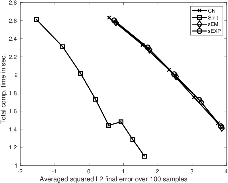
In this numerical experiment, we compare the computational costs of the above time integrators (expect the classical Euler–Maruyama scheme). To do this, we consider the SPDE (1) with the above nonlocal interaction potential for times . We discretize this SPDE using Fourier modes in space. We run samples for each numerical scheme. For each scheme and each sample, we run several time steps and compare the error at the final time with a reference solution provided for the same sample by the same scheme for a very small time-step . Figure 5 displays the total computational time for all the samples, for each numerical scheme and each time-step, as a function of the averaged final error. One observes better performance for the splitting scheme.
Proof of Proposition 4
This appendix provides the proofs of properties of the exact solution to (1).
Global well-posedness. Let Assumption 1 be satisfied. Since the nonlinearity is only locally Lipschitz continuous, a truncation argument is used to prove global well-posedness. Let us stress that the key property of (1) used in the argument below is the fact that is real-valued.
Let be a compactly supported Lipschitz continuous function, such that for . For any , set and . The mapping is globally Lipschitz continuous, and the SPDE
with initial condition , thus admits a unique global solution denoted by . Since the mapping is real-valued, the trace formula holds, see (10): indeed, one obtains
Taking expectation, one obtains the trace formula
where the right-hand side does not depend on truncation index . Using the Burkholder–Davis–Gundy inequality, one obtains
where one observes that does not depend on , using the trace formula above for the term in the integral .
Setting the truncation argument is then straightforward. Let . If , then for all , by construction of . This allows us to define solving (1) for all , where . Finally, almost surely, indeed for every , one has
using the moment estimate above. This concludes the proof of the global well-posedness of (1).
Moment estimates in . Next, let us prove the moment bounds for the exact solution to (1). We provide details only for the moment estimates in the norm (under Assumption 1)
Indeed, the moment estimates for the norm, namely
can either be obtained using similar arguments, or be deduced from the exponential moment estimates for which a detailed proof is provided above. Likewise, the proof of moment estimates
under Assumption 2 would follow from similar arguments.
Let us first consider for all . Its first and second order derivatives are given by
for . Using Itô’s formula, one gets
The first term in the last equality vanishes, and when taking expectation the third term also vanishes. Using the condition (4) to deal with the second term, one obtains
where is a polynomial mapping, see equation (4). Note that one has the upper bound due to moment bounds in the norm. Using the Gronwall Lemma then yields
Let , then applying Itô’s formula for yields
using (4) and Young’s inequality. Using Gronwall’s lemma then concludes the proof of the moment bounds in the norm.
Temporal regularity. It remains to deal with the temporal regularity estimate. Using the mild formulation (2), for any , one has
Using Lemma 1, the first estimate of (4) and the moment bounds in the and norms, one obtains
Using Itô’s isometry formula and Lemma 1, one has
Since the stochastic integrals have Gaussian distribution, gathering the estimates above yields
for all and . This concludes the proof of Proposition 4.
Acknowledgements
We thank André Berg (Umeå University) for discussions on the implementation of Figure 4. The work of CEB was partially supported by the SIMALIN project ANR-19-CE40-0016 of the French National Research Agency. The work of DC was partially supported by the Swedish Research Council (VR) (projects nr. 2018-04443). Part of the work of CEB was carried out when working at Institut Camille Jordan, CNRS and Université Lyon 1. Part of the work of DC was carried out when working for the Department of Mathematics and Mathematical Statistics at Umeå University. The computations were performed on resources provided by the Swedish National Infrastructure for Computing (SNIC) at HPC2N, Umeå University and at Chalmers Centre for Computational Science and Engineering.
References
- [1] M. Ableidinger and E. Buckwar. Splitting integrators for the stochastic Landau-Lifshitz equation. SIAM J. Sci. Comput., 38(3):A1788–A1806, 2016.
- [2] G. Agrawal. Nonlinear Fiber Optics. Electronics & Electrical. Elsevier Science, 2007.
- [3] A. Alamo and J. M. Sanz-Serna. A technique for studying strong and weak local errors of splitting stochastic integrators. SIAM J. Numer. Anal., 54(6):3239–3257, 2016.
- [4] C. A. Anton, Y. S. Wong, and J. Deng. Symplectic schemes for stochastic Hamiltonian systems preserving Hamiltonian functions. Int. J. Numer. Anal. Model., 11(3):427–451, 2014.
- [5] Rikard Anton and David Cohen. Exponential integrators for stochastic Schrödinger equations driven by Itô noise. J. Comput. Math., 36(2):276–309, 2018.
- [6] W. Auzinger, T. Kassebacher, O. Koch, and M. Thalhammer. Convergence of a Strang splitting finite element discretization for the Schrödinger-Poisson equation. ESAIM Math. Model. Numer. Anal., 51(4):1245–1278, 2017.
- [7] W. Bao, S. Jiang, Q. Tang, and Y. Zhang. Computing the ground state and dynamics of the nonlinear Schrödinger equation with nonlocal interactions via the nonuniform FFT. J. Comput. Phys., 296:72–89, 2015.
- [8] Viorel Barbu and Michael Röckner. A splitting algorithm for stochastic partial differential equations driven by linear multiplicative noise. Stoch. Partial Differ. Equ. Anal. Comput., 5(4):457–471, 2017.
- [9] Claude Bardos, Laszlo Erdős, François Golse, Norbert Mauser, and Horng-Tzer Yau. Derivation of the Schrödinger-Poisson equation from the quantum -body problem. C. R. Math. Acad. Sci. Paris, 334(6):515–520, 2002.
- [10] M. Barton-Smith, A. Debussche, and L. Di Menza. Numerical study of two-dimensional stochastic NLS equations. Numer. Methods Partial Differential Equations, 21(4):810–842, 2005.
- [11] Christian Bayer and Harald Oberhauser. Splitting methods for SPDEs: from robustness to financial engineering, optimal control, and nonlinear filtering. In Splitting methods in communication, imaging, science, and engineering, Sci. Comput., pages 499–539. Springer, Cham, 2016.
- [12] André Berg, David Cohen, and Guillaume Dujardin. Lie-Trotter splitting for the nonlinear stochastic Manakov system. J. Sci. Comput., 88(1):Paper No. 6, 31, 2021.
- [13] C. Besse, B. Bidégaray, and S. Descombes. Order estimates in time of splitting methods for the nonlinear Schrödinger equation. SIAM J. Numer. Anal., 40(1):26–40, 2002.
- [14] Christophe Besse, Stéphane Descombes, Guillaume Dujardin, and Ingrid Lacroix-Violet. Energy-preserving methods for nonlinear Schrödinger equations. IMA J. Numer. Anal., 41(1):618–653, 2021.
- [15] S. Blanes and F. Casas. A concise introduction to geometric numerical integration. Monographs and Research Notes in Mathematics. CRC Press, Boca Raton, FL, 2016.
- [16] S. Blanes and P. C. Moan. Splitting methods for the time-dependent Schrödinger equation. Phys. Lett. A, 265(1-2):35–42, 2000.
- [17] N. Bou-Rabee and H. Owhadi. Stochastic variational integrators. IMA J. Numer. Anal., 29(2):421–443, 2009.
- [18] Nawaf Bou-Rabee and Houman Owhadi. Long-run accuracy of variational integrators in the stochastic context. SIAM J. Numer. Anal., 48(1):278–297, 2010.
- [19] Charles-Edouard Bréhier and David Cohen. Strong rates of convergence of a splitting scheme for Schrödinger equations with nonlocal interaction cubic nonlinearity and white noise dispersion. SIAM/ASA J. Uncertain. Quantif., 10(1):453–480, 2022.
- [20] Charles-Edouard Bréhier, David Cohen, and Tobias Jahnke. Splitting integrators for stochastic Lie–Poisson systems. Submitted, 2021.
- [21] Charles-Edouard Bréhier, Jianbo Cui, and Jialin Hong. Strong convergence rates of semidiscrete splitting approximations for the stochastic Allen-Cahn equation. IMA J. Numer. Anal., 39(4):2096–2134, 2019.
- [22] Charles-Edouard Bréhier and Ludovic Goudenège. Weak convergence rates of splitting schemes for the stochastic Allen-Cahn equation. BIT, 60(3):543–582, 2020.
- [23] Franco Brezzi and Peter A. Markowich. The three-dimensional Wigner-Poisson problem: existence, uniqueness and approximation. Math. Methods Appl. Sci., 14(1):35–61, 1991.
- [24] Charles-Edouard Bréhier, David Cohen, and Giuseppe Giordano. Splitting schemes for fitzhugh–nagumo stochastic partial differential equations, 2022.
- [25] Evelyn Buckwar, Adeline Samson, Massimiliano Tamborrino, and Irene Tubikanec. A splitting method for SDEs with locally Lipschitz drift: illustration on the FitzHugh-Nagumo model. Appl. Numer. Math., 179:191–220, 2022.
- [26] K. Burrage and P. M. Burrage. Low rank Runge-Kutta methods, symplecticity and stochastic Hamiltonian problems with additive noise. J. Comput. Appl. Math., 236(16):3920–3930, 2012.
- [27] C. Chen and J. Hong. Symplectic Runge-Kutta semidiscretization for stochastic Schrödinger equation. SIAM J. Numer. Anal., 54(4):2569–2593, 2016.
- [28] Chuchu Chen, Jialin Hong, and Andreas Prohl. Convergence of a -scheme to solve the stochastic nonlinear Schrödinger equation with Stratonovich noise. Stoch. Partial Differ. Equ. Anal. Comput., 4(2):274–318, 2016.
- [29] Chuchu Chen, Jialin Hong, and Xu Wang. Approximation of invariant measure for damped stochastic nonlinear Schrödinger equation via an ergodic numerical scheme. Potential Anal., 46(2):323–367, 2017.
- [30] D. Cohen. Conservation properties of numerical integrators for highly oscillatory Hamiltonian systems. IMA J. Numer. Anal., 26(1):34–59, 2006.
- [31] D. Cohen, J. Cui, J. Hong, and L. Sun. Exponential integrators for stochastic Maxwell’s equations driven by Itô noise. J. Comput. Phys., 410:109382, 2020.
- [32] D. Cohen and L. Gauckler. One-stage exponential integrators for nonlinear Schrödinger equations over long times. BIT, 52(4):877–903, 2012.
- [33] D. Cohen, L. Gauckler, E. Hairer, and Ch. Lubich. Long-term analysis of numerical integrators for oscillatory Hamiltonian systems under minimal non-resonance conditions. BIT, 55(3):705–732, 2015.
- [34] D. Cohen, E. Hairer, and Ch. Lubich. Conservation of energy, momentum and actions in numerical discretizations of non-linear wave equations. Numer. Math., 110(2):113–143, 2008.
- [35] D. Cohen and G. Vilmart. Drift-preserving numerical integrators for stochastic Poisson systems. Int. J. Comput. Math., 0(0):1–17, 2021.
- [36] David Cohen, Jianbo Cui, Jialin Hong, and Liying Sun. Exponential integrators for stochastic Maxwell’s equations driven by Itô noise. J. Comput. Phys., 410:109382, 21, 2020.
- [37] David Cohen, Stig Larsson, and Magdalena Sigg. A trigonometric method for the linear stochastic wave equation. SIAM J. Numer. Anal., 51(1):204–222, 2013.
- [38] Sonja Cox and Jan van Neerven. Convergence rates of the splitting scheme for parabolic linear stochastic Cauchy problems. SIAM J. Numer. Anal., 48(2):428–451, 2010.
- [39] Jianbo Cui. Explicit numerical methods for high dimensional stochastic nonlinear schrödinger equation: Divergence, regularity and convergence, 2021.
- [40] Jianbo Cui and Jialin Hong. Analysis of a splitting scheme for damped stochastic nonlinear Schrödinger equation with multiplicative noise. SIAM J. Numer. Anal., 56(4):2045–2069, 2018.
- [41] Jianbo Cui, Jialin Hong, and Zhihui Liu. Strong convergence rate of finite difference approximations for stochastic cubic Schrödinger equations. J. Differential Equations, 263(7):3687–3713, 2017.
- [42] Jianbo Cui, Jialin Hong, Zhihui Liu, and Weien Zhou. Strong convergence rate of splitting schemes for stochastic nonlinear Schrödinger equations. J. Differential Equations, 266(9):5625–5663, 2019.
- [43] Jianbo Cui, Jialin Hong, and Liying Sun. Structure-preserving splitting methods for stochastic logarithmic schrödinger equation via regularized energy approximation, 2021.
- [44] A. de Bouard and A. Debussche. A stochastic nonlinear Schrödinger equation with multiplicative noise. Comm. Math. Phys., 205(1):161–181, 1999.
- [45] A. de Bouard and A. Debussche. On the effect of a noise on the solutions of the focusing supercritical nonlinear Schrödinger equation. Probab. Theory Related Fields, 123(1):76–96, 2002.
- [46] A. de Bouard and A. Debussche. The stochastic nonlinear Schrödinger equation in . Stochastic Anal. Appl., 21(1):97–126, 2003.
- [47] A. De Bouard and A. Debussche. A semi-discrete scheme for the stochastic nonlinear Schrödinger equation. Numer. Math., 96(4):733–770, 2004.
- [48] A. de Bouard and A. Debussche. Weak and strong order of convergence of a semidiscrete scheme for the stochastic nonlinear Schrödinger equation. Appl. Math. Optim., 54(3):369–399, 2006.
- [49] A. de Bouard, A. Debussche, and L. Di Menza. Theoretical and numerical aspects of stochastic nonlinear Schrödinger equations. Monte Carlo Methods Appl., 7(1-2):55–63, 2001. Monte Carlo and probabilistic methods for partial differential equations (Monte Carlo, 2000).
- [50] Anne de Bouard and Arnaud Debussche. Blow-up for the stochastic nonlinear Schrödinger equation with multiplicative noise. Ann. Probab., 33(3):1078–1110, 2005.
- [51] A. Debussche and L. Di Menza. Numerical simulation of focusing stochastic nonlinear Schrödinger equations. Phys. D, 162(3-4):131–154, 2002.
- [52] R. Duboscq and R. Marty. Analysis of a splitting scheme for a class of random nonlinear partial differential equations. ESAIM Probab. Stat., 20:572–589, 2016.
- [53] G. Dujardin and E. Faou. Qualitative behavior of splitting methods for the linear Schrödinger equation in molecular dynamics. In CANUM 2006—Congrès National d’Analyse Numérique, volume 22 of ESAIM Proc., pages 234–239. EDP Sci., Les Ulis, 2008.
- [54] L. Gauckler. Numerical long-time energy conservation for the nonlinear Schrödinger equation. IMA J. Numer. Anal., 37(4):2067–2090, 2017.
- [55] L. Gauckler and Ch. Lubich. Splitting integrators for nonlinear Schrödinger equations over long times. Found. Comput. Math., 10(3):275–302, 2010.
- [56] François Golse, Clément Mouhot, and Thierry Paul. On the mean field and classical limits of quantum mechanics. Comm. Math. Phys., 343(1):165–205, 2016.
- [57] W. Grecksch and H. Lisei. Approximation of stochastic nonlinear equations of Schrödinger type by the splitting method. Stoch. Anal. Appl., 31(2):314–335, 2013.
- [58] E. Hairer, Ch. Lubich, and G. Wanner. Geometric numerical integration, volume 31 of Springer Series in Computational Mathematics. Springer, Heidelberg, 2010. Structure-preserving algorithms for ordinary differential equations, Reprint of the second (2006) edition.
- [59] R.H. Hardin and F.D. Tappert. Applications of the split-step fourier method to the numerical solution of nonlinear and variable coefficient wave equations. SIAM Review 15, page 423, 1973.
- [60] P. Harms and M. S. Müller. Weak convergence rates for stochastic evolution equations and applications to nonlinear stochastic wave, HJMM, stochastic Schrödinger and linearized stochastic Korteweg–de Vries equations. Z. Angew. Math. Phys., 70(1):Art. 16, 28, 2019.
- [61] J. Hong, L. Miao, and L. Zhang. Convergence analysis of a symplectic semi-discretization for stochastic NLS equation with quadratic potential. Discrete Contin. Dyn. Syst. Ser. B, 24(8):4295–4315, 2019.
- [62] Jialin Hong, Baohui Hou, and Liying Sun. Energy-preserving fully-discrete schemes for nonlinear stochastic wave equations with multiplicative noise. J. Comput. Phys., 451:Paper No. 110829, 20, 2022.
- [63] Martin Hutzenthaler and Arnulf Jentzen. On a perturbation theory and on strong convergence rates for stochastic ordinary and partial differential equations with nonglobally monotone coefficients. Ann. Probab., 48(1):53–93, 2020.
- [64] Reinhard Illner, Paul F. Zweifel, and Horst Lange. Global existence, uniqueness and asymptotic behaviour of solutions of the Wigner-Poisson and Schrödinger-Poisson systems. Math. Methods Appl. Sci., 17(5):349–376, 1994.
- [65] Vladimir V. Konotop and Luis Vázquez. Nonlinear random waves. World Scientific Publishing Co., Inc., River Edge, NJ, 1994.
- [66] B. Leimkuhler and S. Reich. Simulating Hamiltonian dynamics, volume 14 of Cambridge Monographs on Applied and Computational Mathematics. Cambridge University Press, Cambridge, 2004.
- [67] Ben Leimkuhler and Charles Matthews. Molecular dynamics. With deterministic and stochastic numerical methods, volume 39 of Interdisciplinary Applied Mathematics. Springer, Cham, 2015.
- [68] J. Liu. A mass-preserving splitting scheme for the stochastic Schrödinger equation with multiplicative noise. IMA J. Numer. Anal., 33(4):1469–1479, 2013.
- [69] Jie Liu. A mass-preserving splitting scheme for the stochastic Schrödinger equation with multiplicative noise. IMA J. Numer. Anal., 33(4):1469–1479, 2013.
- [70] Jie Liu. Order of convergence of splitting schemes for both deterministic and stochastic nonlinear Schrödinger equations. SIAM J. Numer. Anal., 51(4):1911–1932, 2013.
- [71] Ch. Lubich. On splitting methods for Schrödinger-Poisson and cubic nonlinear Schrödinger equations. Math. Comp., 77(264):2141–2153, 2008.
- [72] R. Marty. On a splitting scheme for the nonlinear Schrödinger equation in a random medium. Commun. Math. Sci., 4(4):679–705, 2006.
- [73] Renaud Marty. Local error of a splitting scheme for a nonlinear Schrödinger-type equation with random dispersion. Commun. Math. Sci., 19(4):1051–1069, 2021.
- [74] R. I. McLachlan and G. R. W. Quispel. Splitting methods. Acta Numer., 11:341–434, 2002.
- [75] A. Millet, S. Roudenko, and K. Yang. Behavior of solutions to the 1D focusing stochastic -critical and supercritical nonlinear Schrödinger equation with space-time white noise. arXiv, 2020.
- [76] G. N. Milstein, Yu. M. Repin, and M. V. Tretyakov. Symplectic integration of Hamiltonian systems with additive noise. SIAM J. Numer. Anal., 39(6):2066–2088, 2002.
- [77] Tetsuya Misawa. A Lie algebraic approach to numerical integration of stochastic differential equations. SIAM J. Sci. Comput., 23(3):866–890, 2001.
- [78] Joshua L. Padgett and Qin Sheng. Convergence of an operator splitting scheme for abstract stochastic evolution equations. In Advances in mathematical methods and high performance computing, volume 41 of Adv. Mech. Math., pages 163–179. Springer, Cham, 2019.
- [79] C. Sulem and P.-L. Sulem. The nonlinear Schrödinger equation, volume 139 of Applied Mathematical Sciences. Springer-Verlag, New York, 1999. Self-focusing and wave collapse.