Large deviations of the ballistic Lévy walk model
Abstract
We study the ballistic Lévy walk stemming from an infinite mean traveling time between collision events. Our study focuses on the density of spreading particles all starting from a common origin, which is limited by a ‘light’ cone . In particular we study this density close to its maximum in the vicinity of the ‘light’ cone. The spreading density follows the Lamperti-arcsine law describing typical fluctuations far from the ‘light’ cone. However this law blows up in the vicinity of the ‘light’ cone horizon which is nonphysical, in the sense that any finite time observation will never diverge. We claim that one can find two laws for the spatial density, the first one is the mentioned Lamperti-arcsine law describing the central part of the distribution and the second is an infinite density illustrating the dynamics for large . We identify the relationship between a large position and the longest traveling time describing the single big jump principle. From the renewal theory we find that the distribution of rare events of the position is related to the derivative of the average of the number of renewals at a short ‘time’ using a rate formalism.
pacs
02. 50. -r, 05. 20. -y, 05. 40. -aI Introduction
The diffusion equation describes the spreading of Brownian particles in a medium Einstein1905Uber; Smoluchowski1906Zur; Metzler2000random. For a packet starting on the origin, the spreading packet is Gaussian which is in agreement with the central limit theorem. Naively, this theory predicts a non-zero probability for a particle starting in say Jerusalem to be found in Tokyo in a split of a second. While this would be a rare event, it is in violation of causality. This problem was solved long time ago with the introduction of the telegraph equation Davydov1934Uravneniya; Goldstein1951diffusion; Joseph1989Heat; Masoliver1996Finite; Weiss2002Some; Bakunin2003Mysteries; Masoliver2017Continuous; Zaburdaev2015Levy. Here, the particle in one dimension at position with time is restricted to a ‘light’ or ballistic cone where is the typical speed (see Fig. 1). The telegraph equation and its extensions to fractional telegraph equations are well studied Compte1997generalized; Eckstein1999mathematics; Cascaval2002Fractional; Qi2011Solutions; Fedotov2016Single; Awad2019On.
Another well investigated problem is the Lévy flight Zumofen1993Scale; Fogedby1994Levy; Shlesinger1995Levy. In one dimension this random walk model deals with the sum of spatial displacements all drawn from a typically symmetric distribution which is fat tailed. The variance is infinite indicating that the Lévy type of central limit theorem is applicable. This process can be described by a fractional space diffusion equation with Metzler2000random; Kessler2012Theory. Similar to the usual diffusion equation, the Lévy flight and its corresponding fractional space diffusion equation suffer from the same deficiency. Here, small and large displacements are assumed all to take place in a unit of time. But this is nonphysical in most cases. In particular, the infinite mean squared displacement predicted by these theories is non-realistic.
The solution to this problem is the introduction of the well-known and widely applicable Lévy walk Shlesinger1982Random; Klafter1994Levy; Zaburdaev2011Perturbation; Zaburdaev2013Space; Ramos2004Levy; Zaburdaev2015Levy; Ariel2015Swarming; Magdziarz2016Explicit; Zaburdaev2016Superdiffusive; Fedotov2016Single; Marcin2017Aging; Fouxon2017Limit; Song2018Neuronal; Giona2019Age; Bologna2020Distribution; Extended2020Giona; Kanazawa2020Loopy, where a finite velocity is introduced. Again, for particles starting on the origin we have a ballistic cone . The mean squared displacement being not faster than ballistic is in agreement with common sense physics. Here, the main point of the Lévy walk model is the coupling between the walking time (or time of walk or traveling time) and the spatial displacement. Unlike the Lévy flight, the stretch of the displacement is connected to its time cost, i.e., the walker has a finite velocity.
Here, we focus on the ballistic phase of the Lévy walk model’ dynamics and the density of spreading particles . In this case the Lamperti-arcsine Margolin2005Nonergodicity; Froemberg2015Asymptotic distribution describes the shape of the distribution of propagating particles in the long time limit (see below). In some sense, this distribution replaces the more familiar Gaussian and Lévy distributions describing Brownian motion and Lévy flight. The Lamperti-arcsine distribution has a U or W shape (see below). It means that in this scaling limit diverges when (but always ). The conclusion from this behavior is apparent. The divergence of the Lamperti-arcsine scaling solution is unphysical, in the sense that for any finite time we cannot obtain a blow up of the density, and this problem is cured here. In other words: the study of rare events is important. Hence, we set out to find the corrections and the accurate description of the Lévy walk. Here the central part of describes what we call typical or bulk fluctuations while its behavior close to the ballistic cone is a rare event regime, to be defined more precisely later. To summarize, while the telegraph equation solves the nonphysical behaviour presented in the diffusion approximation and the Lévy walk corrects the nonphysical nature of the Lévy flight, we focus on the nonphysical blow up of Lamperti-arcsine solutions of the ballistic Lévy walk. For schematics, see Fig. 1.
We emphasize that previous works in the field are technically correct in the long-time limit . However, for large clear finite time effects are found here. And the rare event corrections are found when the particle distribution attains its maximum. In this sense, we are dealing with a vastly different case compared to the telegraph equation which provides for large where the probability is small at least for long times; see Fig. 1. Our treatment of rare events of the ballistic Lévy walk is based on the so called infinite covariant densities Aaronson1997introduction; Rebenshtok2014Infinite; Rebenshtok2014Non; Erez2017Large; Wang2018Renewal; Erez2019From; Wang2019Ergodic and the big jump principle Cistjakov1964theorem; Alessandro2019Single; Wang2019Transport. Both techniques are directly related (see below) and cure the nonphysical behaviour of Lamperti-arcsine solution in the vicinity of their maximum. This problem was already treated for the Lévy walk with finite mean traveling times using several approaches Fouxon2017Limit; Alessandro2019Single; Vezzani2020Rare.
The remainder of the manuscript is organized as follows. In Sec. II, we outline the Lévy walk model. We study the difference between typical fluctuations and rare events, and compare them with simulations in Sec. III. In Sec. IV, we build the relationship between the position of the particle and the longest waiting time, exposing the big jump principle Alessandro2019Single for the studied case. The relation between rare events of the position and the averaged number, and the propagator are considered in Secs. V and VI. Finally, we conclude with a discussion.

II Model
II.1 Renewal process and Lévy walk model
We first outline the main ingredients of the renewal process Feller1971introduction; Godreche2001Statistics; Godreche2015Statistics; Wang2018Renewal and Lévy walk model. The former is defined as follows: Events happen at the random epochs of time , , , , , from some time origin . Here we suppose time intervals , , , , , are independent and identically distributed (IID) random variables with a common PDF . These -s are called walking times (sometimes also flight times or traveling times). Thus, the considered process is a renewal process. Given that the number of renewals during is , i.e., , the corresponding observation time is
| (1) |
Here , defined by , is the time interval between the time and the last event before . When is fixed, our is a random variable.
We further consider the Lévy walk model in which the directions of each step are introduced. The particles move continuously with a constant velocity for a random time drawn from a PDF . Here the directions of particles, i.e., or , are chosen randomly with equal probability. The corresponding displacement is () on condition that the direction of the first step is negative (positive). We further generate another waiting time from and the direction of the particle. Then the process is renewed. Here as mentioned are IID random variables with a common PDF . We are interested in the position of the particle at time
| (2) |
where are the displacement of step and is the last displacement. Notice that is the position of the particle at time while is the displacement of the particle for a single step. Similar, describes the observation time of the process but is the time of walk or traveling time drawn from . Below we will show how to derive the distribution of . Clearly the particles starting on the origin are all within the ‘light’ cone .
II.2 Propagator of Lévy walk
Let us briefly recap the basic equations of the model considered in this paper. For the velocity model under study, the particle moves continuously with a constant velocity and changes directions at random times Klafter1987Stochastic; Zaburdaev2015Levy. Mathematically, the joint probability of the step’s length and duration time is
| (3) |
The above equation describes the probability to move a distance in time with a single event and accounts for the space-time correlation. The PDF of the particle’s position at time is governed by Zumofen1993Scale
| (4) |
and the PDF of the particle’s position reads
| (5) |
where
is the probability of moving a distance in time in a single motion during the last uncompleted step with , and is probability of just arriving at at time after completing a step. In Eqs. (4, 5) we identify the convolution both in time and in space, hence the analysis proceeds with Laplace-Fourier transforms. Combining Eqs. (4) and (5) yields Klafter1987Stochastic; Zaburdaev2015Levy
| (6) |
where is the Fourier and Laplace transforms of . Such equations are known as Montroll-Weiss equations, they are not generally easy to invert, and hence later we turn to the asymptotic analysis.
II.3 Three types of distributions of waiting times
In our analysis, we use the power law distribution of the times of walk capturing a heavy tail Peter1990Reaction; Bouchaud1990Anomalous; Metzler2000random; Fernando2009Beyond; Tameem2017Temperature
| (7) |
with for large . In Laplace space, from the Tauberian theorem Feller1971introduction and Eq. (7) we have
| (8) |
with . Here is a constant determined by the details of . In this paper we denote as the Laplace transform of and is conjugate to . We have , since is a normalized density. Below we consider the exact forms of three types of waiting time PDFs with the same heavy-tails, which will be used to show the features of typical fluctuations and rare fluctuations.
II.3.1 Pareto distribution
Our first example is called the Pareto distribution Klafter2011First. It is defined as follows
| (9) |
When , the first moment of is divergent. Note that for Eq. (9), we have according to Tauberian theorem.
II.3.2 One-sided Lévy distribution
II.3.3 Mittag-Leffler distribution
Another density of the walking time is the Mittag-Leffler PDF Podlubny1999Fractional; Kozubowski2001Fractional; Vainstein2006Non; Oliveira2019Anomalous, i.e.,
| (12) |
with being the Mittag-Leffler function defined by
| (13) |
In Laplace space, has the specific form
| (14) |
The Mittag-Leffler distribution is a geometric stable distribution Kozubowski2001Fractional. When , we have .
II.4 Rare events versus typical fluctuations
For , the average of the waiting time diverges, which leads to ballistic-diffusion Klafter1994Levy, namely with . The infinite mean traveling time is responsible for the ballistic Lévy walk characterized by the ballistic front. Note that also Generalised Langevin equation, under certain conditions, yields ballistic diffusion, however since the noise in this equation is assumed Gaussian both the typical and rare events are normal Vainstein2006Non; Oliveira2019Anomalous. In Froemberg2015Asymptotic, the typical fluctuations were discussed in detail, i.e., the position is of the order of . When , the distribution of the position follows the arcsine law Lamperti1958occupation; Froemberg2015Asymptotic
| (15) |
with . Clearly, the arcsine law works very well for the central part of the distribution of the position both for one-sided Lévy distribution and Pareto distribution; see the red solid line in Fig. 2 (a). Due to the variable transformation, and are related by . While, when or , the typical fluctuations Eq. (15) blow up which is nonphysical at least for a finite time . This drawback of the arcsine law, i.e., the nonphysical divergence at in the vicinity of the ballistic cone, is circumvented in this paper when a second type of scaling of the density is considered. See the data circled in red on the bottom panel of Fig. 2. It implies that under certain conditions the density of the position is characterized by two scaling laws. The first one is the mentioned normalized arcsine law Eq. (15) describing the scaling when but . Note that the central limit theorem (Lamperti-arcsine form) describes the central part of the distribution, but for finite though large it does not describe the rare fluctuations, i.e., large behavior. An important feature of the typical fluctuations is that its behavior is universal which is only determined by the far tail of the waiting time PDF, namely, Eqs. (9, 10) and (12), are not vitally important for the typical fluctuations on condition that they have the same heavy-tails governed by the index .
The second scaling corresponds to the non-normalized state showing the behavior of the density for , which is described by infinite densities Aaronson1997introduction; Rebenshtok2014Infinite; Rebenshtok2014Non; Erez2017Large; Wang2018Renewal; Erez2019From; Wang2019Ergodic. Here our aim is to find the statistics of rare fluctuations , where the detailed structure of the waiting time PDF is of importance.

III Results for Lévy walk
III.1 Bulk fluctuations
First, we focus on the typical fluctuations, namely the case and both are large, implying that and are small and comparable. Inserting Eq. (8) into Eq. (6), we get
with
It can be seen that the above equation is normalized since . The inverse Fourier-Laplace transform for the expression can be performed exactly following the methods given in Refs. Godreche2001Statistics; Froemberg2015Asymptotic, which yields the description of what we call bulk or typical fluctuations Margolin2005Nonergodicity; Froemberg2015Asymptotic; Magdziarz2016Explicit
| (16) |
with the scaling form . Here as usual, the subscript means that is the corresponding PDF of . The propagator Eq. (16) is called the Lamperti distribution Lamperti1958occupation. Here since , namely there exists a finite ‘light’ cone in which we may find the particle. The second moment of the position is , which corresponds to a ballistic behavior Klafter1994Levy; Froemberg2015Asymptotic. When , Eq. (16) reduces to Eq. (15) which is plotted in Fig. 2, and as expected describes well the central part of the packet of spreading particles. A related expression is
| (17) |
with which is plotted by the dashed line in Fig. 3. There when is small, we identify the deviations from the arcsine law.
III.2 Rare fluctuations
We consider the case of using the random variable where is small. In Fourier-Laplace spaces, the density of becomes
| (18) |
Here is the Fourier pair of the shifted position . Utilizing Eqs. (6) and (18), we get
| (19) |
We are interested in analyzing the behavior of the position in the long time regime (), where and are sufficient small and large, respectively. Using Eq. (8), Eq. (19) reduces to a simple expression
| (20) |
Note that the inverse Laplace transform of gives a delta function which is ignored and not related to our long time behavior. Here, we stress that Eq. (20) is valid in the limit of and . In other words, Eq. (20) can not yield an effective prediction for . See further discussion below. Taking the inverse Laplace-Fourier transform of Eq. (20) gives the main result of this section
| (21) |
with
| (22) |
Here we used the fact that and are Laplace pairs. As mentioned before the time-dependent Eq. (21) is valid in the limit of . The theoretical prediction Eq. (21) with being the one-sided Lévy distribution is plotted in Fig. 3 by using the numerical inverse Fourier transform. The comparison to numerical simulation is excellent, while the arcsine law completely fails to describe the observed behavior. It can be seen that given in Eq. (22) is an infinite density since , namely the is not normalised, which is hardly surprising since it is obtained from a normalised density multiplied by hence the area under the left hand side of Eq. (21) is obviously diverging.
Let us consider three examples:
i) For the Pareto distribution, we can not invert Eq. (21) exactly, however we may invert it numerically. While, there is a simply way by considering the limit . Using and taking the inverse Fourier transform gives
| (23) |
If we are only interested in the behavior of , the second term works perfectly and Eq. (23) reduces to
| (24) |
with . Note that Eq. (24) in the limit is valid for a large range of PDFs, for example the mentioned Mittag-Leffler and the one-sided Lévy distributions.
ii) For the one-sided Lévy distribution, we use the geometric series and get by inversion
| (25) |
where is the Lévy PDF Metzler2000random, defined by
| (26) |
When or , only the function is of importance. As expected, Eq. (21) reduces to the survival probability, describing the probability of moving in the same direction for the whole observation time . On the contrary, the function loses its role for or .
iii) For the Mittag-Leffler distribution, using Eq. (14), it is easy to show
| (27) |
Utilizing Eqs. (27) and (21), as , we have
| (28) |
according to the relationship . It indicates that Eq. (28) agrees with the far tail of the Lamperti distribution Eq. (16) in the limit of . Namely, Eq. (28) exhibits a unique behavior that the rare events are described by the same theory as the typical fluctuations; see Fig. 3. Besides, an interesting feature of is exclusively exhibited by the rare events analysis, i.e., a discrete probability describing the survival probability of the particles is found. For the Mittag-Leffler distribution, it is easy to check that Eq. (21) is not normalised. To be more exactly, the divergence happens at .
In Fig. 3, we show the propagator corresponding to Eq. (21) in the scaling form. For , the calculated , Eq. (16), follows reasonably the arcsine law and this is only valid for the central part of the distribution of the position, namely but . As the figure shows, it is difficult to find the difference between the typical fluctuations and the theoretical result with the Mittag-Leffler waiting time statistics, while, if and the waiting time follows the Pareto or the one-sided Lévy distributions, deviations from Eq. (17) are clearly presented. When , the rare events of can be obtained by using the symmetry property of the density and here we did not discuss this in detail. In Fig. 4, the scaling form is exhibited with different observation time to show the properties of the infinite density. Clearly, for small , is independent of the observation time and its shape does not change.


IV Relation between the position and the longest waiting time
An interesting problem is the relation between large behavior of the distribution and the distribution of the longest traveling time in the renewal process. This problem is related to extreme value statistics Gumbel2004Statistics; Albeverio2006Extreme; Majumdar2009Large; Lefevere2011Large; Tsirelson2013uniform; Krapivsky2014Large; Chaitra2014Universal; Mauro2016Large; Hartich2019Extreme; Marc2019. Extreme events are natural phenomena and play an important role in our life. Thus, it is important to study how these rare events are related to other observables. Here, we wish to establish a connection between the longest time of walk and the position of the particle. Such relations are based on the well-known big jump principle Cistjakov1964theorem; Alessandro2019Single. Mathematically, when are IID random variables with a sub-exponential tail, the single big jump principle is
| (29) |
when is large. Notice that this relationship Eq. (29) is valid for any integer . See related works where this principle was applied in physical systems Thomas2013Precise; Buraczewski2013Large; Wang2019Transport. However here we have a constraint on the time of walk, namely they all sum up to the fixed measurement time . In other words, the traveling times are non IID and Eq. (29) is not directly relevant to our study. We will see that the big jump principle for the ballistic motion is different in comparison to the previously studied case when Alessandro2019Single.
For the well-known IID case, in Eq. (29) is fixed. In our model, is a random variable since ; see Fig. 5. This constraint also implies that we have correlations in the process, though they stem from a renewal process, and hence still can be analysed. Here we must distinguish between two types of rare events. We will focus on being large but strictly . Then in Sec.VI we will treat . The latter gives a delta function contribution to .
Here, we first define
The limiting law of typical fluctuations of has been studied by C. Godrèche et al. in Ref. Godreche2015Statistics. Here we recently showed that another law will be found when the second scaling or is introduced Marc2019. If , the density of can be deduced from the following inverse Fourier transform
| (30) |
with ; see Eq. (56) in Appendix A. We focus on the case where is large and . The limit corresponds to the large ‘time’ . Note that here we must consider the full form of the density, namely is important, while for the typical fluctuations only the small behavior of Eq. (8) is important. Rewriting Eq. (21), for the variable we have
| (31) |
Combining Eqs. (30) and (31), we get the main result of this section
| (32) |
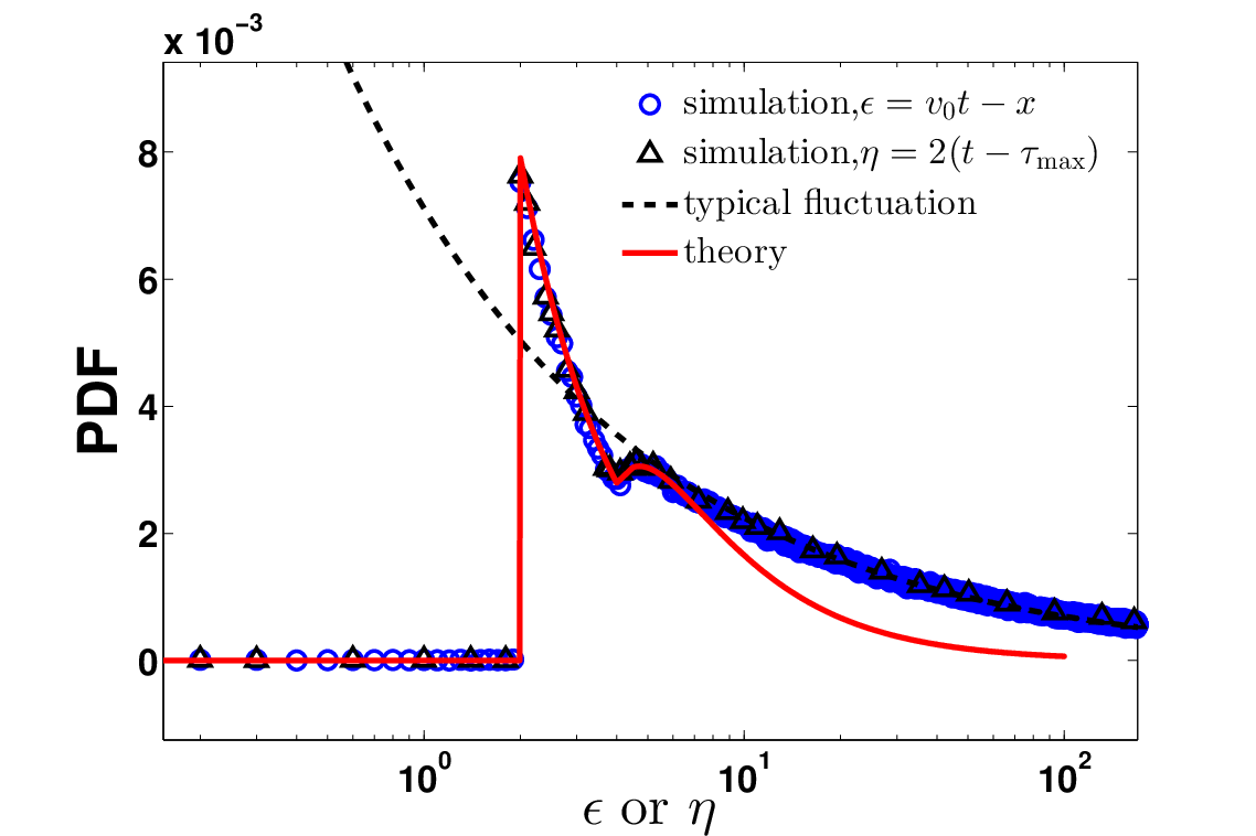
where is large and means that the distributions of the random variables on both sides of Eq. (32), i.e., and , are the same. Hence in Eq. (32) is of course the position of the particle at large , when it is in the vicinity of the ‘light’ cone. As shown in Fig. 6, the density of is consistent with that of for large and . Rewriting Eq. (32) yields
| (33) |
This behavior can be tested based on a correlation plot. As can be seen in Fig. 7, the strong relation between and is illustrated 11 1 In our simulations we do not have the data below the line since which yields .. As expected, we find that grows linearly with for a small .
This relation stressed here is different from the case of discussed in Alessandro2019Single in which the relation is . The reason is as follows: For , the length of the displacement made in , which is the time interval free of the longest waiting time, follows . While, for , the situation is changed since and the term comes into play. See further details in Appendix B.
We further treat Eq. (32) heuristically to explain its meaning. Now the total observation time is divided into two parts: One is the sum of waiting times denoted by when directions of particles are positive and the other one is . We assume that , the particles arrive there by a mechanism of large jump. This means that we have and . More specifically, we consider two random variables and the remaining time . The corresponding position of the particle is . We further suppose that the particle moves with velocity in and in the remaining time, then the position of the particle at time is
| (34) |
If the particle does not change its direction in the mentioned two time intervals, we have (a delta function).
To conclude we see that rare events are obtained by a particle moving only in one direction from Eq. (34) (for ) and reversing direction in the remaining time, we do not see this as an intuitive result, but when is really big the particle is left with little time to reverse, hence the ballistic motion with the reverse direction is plausible (and if it continues in the same direction, we are on the horizon of the walk, which is not considered here). Note that in principle the number of renewals related to Eq. (32) can be a large number and is not limited to one. This will be discussed rigorously in the following section.


V Relation between rare events of the position and the average of renewals
Now the aim is to investigate the relation between and the number of renewals. Note that the rare events of the position are governed by with being a positive integer according to Eqs. (25) and (23). It indicates that the rare events of the position have a strong relationship with the number of renewals. Based on the renewal theory Godreche2001Statistics, in Laplace space (), the probability of the number of renewals during time interval and is Godreche2001Statistics
| (35) |
We can check that is normalized by using . According to Eq. (35), the mean of renewals is
| (36) |
Rewriting Eq. (36), we get
| (37) |
Taking the inverse Laplace transform yields
| (38) |
with . Note that Eq. (38) is the exact result for and ] corresponds to the rate of the number of renewals Takuma2020Infinite. Combining the second line of the right hand side of Eqs. (31) and (38), the relation between the behavior of and is found
| (39) |
Eq. (39) is the main result of this section describing the relation between the position of the Lévy walker and the derivative of the average of the number of renewals at the value of . Thus, we need to observe data only for a very short time and then we can map the observed number of renewals to the rare fluctuations of the position generated for an extremely long observation time . This is particularly important for real experiments to save a lot of time and expense since there is no need to record the data up to observation time . In that sense we find an useful and important relation between positional rare fluctuations and the derivative of . Eq. (39) is illustrated in Fig. 8. Here the right-hand side of Eq. (39) is obtained by averaging realizations. It can be seen that is connected to the average of renewals at a small ‘time’ . The simulations for the mean number of renewals were made only up to time , still they predict the rare events with simulations made for time .

VI Propagator for the Pareto traveling time PDF
Now we deal with a general observation time instead of the long time limit considered in previous sections, then use a different method to explain the rare fluctuations again. Here we focus on the case of the waiting time following the Pareto distribution Eq. (9). Recall that is the cutoff for this distribution. If , from Eq. (24) we get . Indeed in Fig. 3 we see this effect rather easily, however this is an approximation valid in the long time limit only, for finite times this rule is not strictly valid as the probability of finding the particle in this interval is not identically zero. Intuitively, the large position is related to the large waiting time and the large waiting time is determined by the far tail of the waiting time. So it would be interesting to consider the relationship between the far tail of the waiting time and the large position.
Using Taylor’s expansion on Eq. (6), we get
| (40) |
Here the summation over is a sum over the number of renewals, which as mentioned is random. We focus on the case of . If , then clearly the particle is not in the interval under study. In order to obtain in the mentioned spatial interval, we need to consider the propagator Eq. (40). Utilizing the definition of and , for the above equation reduces to
| (41) |
The infinite terms on the right-hand side of Eq. (41) describe the probability of moving in positive direction all the time but the direction of the last step is negative. This is the only way the particles can reach at time . Taking the inverse Laplace-Fourier transform, we obtain
| (42) |
which reduces to
| (43) |
with . When is large, i.e., , we have
| (44) |
Thus,
| (45) |
Clearly, the far tail of the position decays as a power law. Contrary to Eq. (24) with , the behavior of is governed by the far tail of the PDF for a finite time; see Fig. 9. With the increasing of observation time , Eq. (43) goes to zero and approaches Eq. (24) since the probability of reaching becomes smaller and smaller.

We proceed with the discussion of . Recall that for Eq. (32), it is meaningless for . When all directions of the particles are the same, this contributes to the probability of . For this maximum point, we have
| (46) |
with . The inversion of Eq. (46) is
| (47) |
In the long time limit, using , Eq. (47) reduces to
| (48) |
It can be seen that Eq. (48) depends on the initial position of the particle and is related to the survival probability. In reality, Eq. (48) is related to the single big jump principle, namely, the particles go in the one direction for the first step and continue in the same way for the rest steps.
In summary: We have carried out an investigation on the moving forward particles, leading to a delta function contribution at ; see Eq. (48). This is clearly a description of a rare event, hence the theory is developed in two stages, large and comparable to but strictly smaller, and . Note that when , the particle did not change its direction, but the renewal process may have many collision events. If the velocity distribution is not and with equal probability we might obtain different behaviors than what we presented here, however this is hardly surprising as it is also true for the bulk Froemberg2013Random.
One may wonder how can we understand the mechanism of rare fluctuations discussed in previous section. Motivated by the finite time limit Eq. (45), we consider the case that the particle just has only one negative velocity (the rest epochs are positive) to study the behavior of . Similar to Eq. (41), we obtain from Eq. (40)
| (49) |
Here the second line of the right hand side of Eq. (49) corresponds to case where the negative velocity is only in the last step and the first line is when the sole negative direction is not the last one. The sum of the infinite geometric series yields
| (50) |
Using relation Eq. (18) again, we have
| (51) |
The inverse Laplace transform of the above equation gives
| (52) |
Based on Eq. (52), the leading term of Eq. (25) is obtained again in the limit . It can be seen that Eq. (51) or (52) is an exact solution with Eq. (9) when . Besides, it is easy to find that the rare events of the position are closely contact to the number of the negative directions. This is also corresponding to the expanded terms of Eq. (22) in powers of .
VII Conclusion
The main focus of this manuscript has been on the rare fluctuations of the ballistic Lévy walk model in one dimension. We show here that the density in the vicinity of the ballistic cone , is described by the full shape of the distribution of waiting times, unlike the typical fluctuations which are described by the Lamperti-arcsine law. To highlight the rare fluctuations, we use a second non ballistic scaling. Namely, we multiply the PDF with and obtain the infinite density ; see Eqs. (22) and (21). The integral of diverges at large and in that sense it is a non-normalizable solution which is hardly surprising. The infinite density and the normalized Lamperti-arcsine are complementary, with the former describing the positional distribution in the vicinity of the ‘light’ cone, namely close to the maximum of the packet. Certainly, our infinite density is different from the case of Rebenshtok2014Non. We gave the relation between the infinite density of the maximum of waiting times and the infinite density of the position . In this sense we relate between extreme value statistic of constrained random variables () and the position of the Lévy walk close to the ballistic cone. This gives a single big jump principle for the ballistic Lévy walk Eq. (33). We note that this formula differs from the one found in the super-diffusive phase of the Lévy walk model Alessandro2019Single. We also analysed the moving forward particles which lead to a delta function contribution [see Eq. (48)] and are also clearly rare events in the long time limit.
We have developed a rate formalism to the rare events, see Eq. (39). Recently, Akimoto et al. considered a related rate formalism for a different observable: the velocity Takuma2020Infinite, while here we consider the position. Indeed the rate approach is a valuable tool for the calculations of large fluctuations, at least for renewal processes. This rate formalism was initially developed by Vezzani et al Alessandro2019Single; Vezzani2020Rare. In real experiments or simulations with trajectories generated with a computer program, the observation of the rare fluctuations is a challenge, since we need many samples and a long observation time . Here we investigate the rare fluctuations of the position from a new and different point of view. Utilizing the renewal theory, we find that the rare events of the Lévy walk are related to the mean number of renewals in the observation time . This is to say, if we are interested in the rare events of the position of the ballistic Lévy walk model, we just need the data of the renewals at some ‘time’ ; see Eq. (39). And since is of order , the ‘time’ here is actually very short, so the knowledge of the mean number of renewals for short times provides the full information on the rare events for large times, which is remarkable.
Acknowledgments
E. B. acknowledges the Israel Science Foundation for support through Grant No. 1898/17. M.H. is funded by the Deutsche Forschungsgemeinschaft (DFG, German Research Foundation) - 436344834. W.W. thanks Felix Thiel for the discussions. W.W. was supported by Bar-Ilan University together with the Planning and Budgeting Committee fellowship program.
Appendix A Calculation of the PDF of
Let us give a brief account of the statistic of . In Laplace space, the density of satisfies Godreche2015Statistics
| (53) |
with
| (54) |
From Eq. (53), the density of follows
| (55) |
In the limit and , the leading term of Eq. (55) is
| (56) |
Notice that Eq. (56) can be further simplified. Substituting Eq. (8) into Eq. (56) and taking the inverse Laplace transform give
| (57) |
Rewriting Eq. (57) yields the scaling form of
| (58) |
see also Godreche2015Statistics. Let us now take the integral over from to of Eq. (58), we get
| (59) |
It indicates that only , the density is normalized otherwise not. Note that Eq. (57) is valid under condition that and is large . While, when another scaling is introduced, i.e., , the statistics of will be changed. Using the definition of inverse Laplace transform on Eq. (56) gives
| (60) |
When , the random variable tends to infinity and in this limit Eq. (60) corresponds to the statistics of large . While, for we need the information of large rather than . In other words, the dynamic of is governed by the full form of . Here we just use the density of to build the relationship between and , and discussion of Eq. (55) or (56) will be shown by another paper Marc2019.


Appendix B The relation between the largest position and the longest traveling time with
Here we make a brief comparison for the rare events of position and the waiting time. Contrary to , the rare event of the position is not only determined by the longest waiting times but also by another fluctuant term. Though the micro term is small, we can not ignore it; see Eq. (33). This relation can also be found for the case of ; see Figs. 11 and 10 from the view of the distribution and the correlation plot. This means that in some special region near the rare fluctuations are determined by the full form of the waiting time even for . While, with the decrease of , the behavior is governed by the asymptotic behavior of the distribution of the waiting time showing the behavior when but ; see Ref. Alessandro2019Single. As expected, the single big jump principle Eq. (32) under study, will vanish due to with the increase of and . With the help of our work, one can get a better understanding about the rare events, the relation between and , and the infinite densities.
References
- (1) A. Einstein, Ann. Phys. 322, 549 (1905).
- (2) M. von Smoluchowski, Ann. Phys. 326, 756 (1906).
- (3) R. Metzler and J. Klafter, Phys. Rep. 339, 1 (2000).
- (4) D. B. I, DoM. Akad. Nauk SSSR 2, 474 (1934).
- (5) S. Goldstein, Q. J. Mech. Appl. Math. 4, 129 (1951).
- (6) D. D. Joseph and L. Preziosi, Rev. Mod. Phys. 61, 41 (1989).
- (7) J. Masoliver and G. H. Weiss, Eur. J. Phys 17, 190 (1996).
- (8) G. H. Weiss, Physica A 311, 381 (2002).
- (9) O. G. Bakunin, Phys. Usp. 46, 309 (2003).
- (10) J. Masoliver and K. Lindenberg, Eur. Phys. J. B 90, 1 (2017).
- (11) V. Zaburdaev, S. Denisov, and J. Klafter, Rev. Mod. Phys. 87, 483 (2015).
- (12) A. Compte and R. Metzler, J. Phys. A: Math. Gen. 30, 7277 (1997).
- (13) E. C. Eckstein, J. A. Goldstein, and M. Leggas, Electron. J. Differential Equations 1999, 39 (1999).
- (14) R. C. Cascaval, E. C. Eckstein, C. L. Frota, and J. A. Goldstein, J. Math. Anal. Appl. 276, 145 (2002).
- (15) H. Qi and X. Jiang, Physica A 390, 1876 (2011).
- (16) S. Fedotov, Phys. Rev. E 93, 020101(R) (2016).
- (17) E. Awad, Physica A 518, 210 (2019).
- (18) G. Zumofen and J. Klafter, Phys. Rev. E 47, 851 (1993).
- (19) H. C. Fogedby, Phys. Rev. Lett. 73, 2517 (1994).
- (20) M. F. Shlesinger, G. M. Zaslavsky, and U. Frisch (eds.), Lévy flights and related topics in physics, vol. 450 of Lecture Notes in Physics (Springer-Verlag, Berlin, 1995).
- (21) D. A. Kessler and E. Barkai, Phys. Rev. Lett. 108, 230602 (2012).
- (22) M. F. Shlesinger, J. Klafter, and Y. M. Wong, J. Stat. Phys. 27, 499 (1982).
- (23) J. Klafter and G. Zumofen, Phys. Rev. E 49, 4873 (1994).
- (24) V. Zaburdaev, S. Denisov, and P. Hänggi, Phys. Rev. Lett. 106, 180601 (2011).
- (25) V. Zaburdaev, S. Denisov, and P. Hänggi, Phys. Rev. Lett. 110, 170604 (2013).
- (26) G. Ramos-Fernández, J. L. Mateos, O. Miramontes, G. Cocho, H. Larralde, and B. Ayala-Orozco, Behav. Ecol. Sociobiol. 55, 223 (2004).
- (27) G. Ariel, A. Rabani, S. Benisty, J. D. Partridge, R. M. Harshey, and A. Be’er, Nat. Commun. 6, 8396 (2015).
- (28) M. Magdziarz and T. Zorawik, Phys. Rev. E 94, 022130 (2016).
- (29) V. Zaburdaev, I. Fouxon, S. Denisov, and E. Barkai, Phys. Rev. Lett. 117, 270601 (2016).
- (30) M. Magdziarz and T. Zorawik, Phys. Rev. E 95, 022126 (2017).
- (31) I. Fouxon, S. Denisov, V. Zaburdaev, and E. Barkai, J. Phys. A: Math. Theor. 50, 154002 (2017).
- (32) M. S. Song, H. C. Moon, J.-H. Jeon, and H. Y. Park, Nat. Commun. 9, 1 (2018).
- (33) M. Giona, M. D’Ovidio, D. Cocco, A. Cairoli, and R. Klages, J. Phys. A: Math. Theor. 52, 384001 (2019).
- (34) M. Bologna, J. Stat. Mech: Theory Exp. 2020, 073201 (2020).
- (35) M. Giona, A. Cairoli, and R. Klages, ArXiv:2009.13434.
- (36) K. Kanazawa, T. G. Sano, A. Cairoli, and A. Baule, Nature 579, 364 (2020).
- (37) G. Margolin and E. Barkai, Phys. Rev. Lett. 94, 080601 (2005).
- (38) D. Froemberg, M. Schmiedeberg, E. Barkai, and V. Zaburdaev, Phys. Rev. E 91, 022131 (2015).
- (39) J. Aaronson, An Introduction to Infinite Ergodic Theory, vol. 50 of Mathematical Surveys and Monographs (American Mathematical Society, Providence, RI, 1997).
- (40) A. Rebenshtok, S. Denisov, P. Hänggi, and E. Barkai, Phys. Rev. E 90, 062135 (2014).
- (41) A. Rebenshtok, S. Denisov, P. Hänggi, and E. Barkai, Phys. Rev. Lett. 112, 110601 (2014).
- (42) E. Aghion, D. A. Kessler, and E. Barkai, Phys. Rev. Lett. 118, 260601 (2017).
- (43) W. Wang, J. H. P. Schulz, W. H. Deng, and E. Barkai, Phys. Rev. E 98, 042139 (2018).
- (44) E. Aghion, D. A. Kessler, and E. Barkai, Phys. Rev. Lett. 122, 010601 (2019).
- (45) X. Wang, W. Deng, and Y. Chen, J. Chem. Phys. 150, 164121 (2019).
- (46) V. P. Chistjakov, Theory Probab. Appl. 9, 640 (1964).
- (47) A. Vezzani, E. Barkai, and R. Burioni, Phys. Rev. E 100, 012108 (2019).
- (48) W. Wang, A. Vezzani, R. Burioni, and E. Barkai, Phys. Rev. Res. 1, 033172 (2019).
- (49) A. Vezzani, E. Barkai, and R. Burioni, Sci. Rep. 10, 1 (2020).
- (50) W. Feller, An Introduction to Probability Theory and Its Applications. Vol. II. Second edition (John Wiley & Sons, Inc., New York, 1971).
- (51) C. Godrèche and J. M. Luck, J. Stat. Phys. 104, 489 (2001).
- (52) C. Godrèche, S. N. Majumdar, and G. Schehr, J. Stat. Mech: Theory Exp. 2015, P03014 (2015).
- (53) J. Klafter, A. Blumen, and M. F. Shlesinger, Phys. Rev. A 35, 3081 (1987).
- (54) P. Hänggi, P. Talkner, and M. Borkovec, Rev. Mod. Phys. 62, 251 (1990).
- (55) J.-P. Bouchaud and A. Georges, Phys. Rep. 195, 127 (1990).
- (56) F. D. Stefani, J. P. Hoogenboom, and E. Barkai, Phys. Today 62, 34 (2009).
- (57) T. Albash, V. Martin-Mayor, and I. Hen, Phys. Rev. Lett. 119, 110502 (2017).
- (58) J. Klafter and I. M. Sokolov, First Steps in Random Walks: From Tools to Applications (Oxford University Press, Oxford, 2011).
- (59) I. Podlubny, Fractional Differential Equations (Academic Press, Inc., San Diego, 1999).
- (60) T. J. Kozubowski, Math. Comput. Modelling 34, 1023 (2001).
- (61) M. H. Vainstein, I. V. L. Costa, R. Morgado, and F. A. Oliveira, EPL 73, 726 (2006).
- (62) F. A. Oliveira, R. M. S. Ferreira, L. C. Lapas, and M. H. Vainstein, Front. Phys 7, 18 (2019).
- (63) J. Lamperti, Trans. Amer. Math. Soc. 88, 380 (1958).
- (64) E. J. Gumbel, Statistics of Extremes (Dover Publications, Inc., Mineola, 2004).
- (65) S. Albeverio, V. Jentsch, and H. Kantz (eds.), Extreme Events in Nature and Society (Springer, Berlin, 2006).
- (66) S. N. Majumdar and M. Vergassola, Phys. Rev. Lett. 102, 060601 (2009).
- (67) R. Lefevere, M. Mariani, and L. Zambotti, Stoch. Process. Their Appl. 121, 2243 (2011).
- (68) B. Tsirelson, Electron. Comm. Probab. 18 (2013).
- (69) P. L. Krapivsky, K. Mallick, and T. Sadhu, Phys. Rev. Lett. 113, 078101 (2014).
- (70) C. Hegde, S. Sabhapandit, and A. Dhar, Phys. Rev. Lett. 113, 120601 (2014).
- (71) M. Mariani and L. Zambotti, Adv. in Appl. Probab. 48, 648 (2016).
- (72) D. Hartich and A. Godec, J. Phys. A 52, 244001 (2019).
- (73) M. Höll, W. L. Wang, and E. Barkai, ArXiv:2006.06253.
- (74) T. Mikosch and O. Wintenberger, Probab. Theory Related Fields 156, 851 (2013).
- (75) D. Buraczewski, E. Damek, T. Mikosch, and J. Zienkiewicz, Ann. Appl. Probab. 41, 2755 (2013).
- (76) T. Akimoto, E. Barkai, and G. Radons, Phys. Rev. E 101, 052112 (2020).
- (77) D. Froemberg and E. Barkai, Eur. Phys. J. B 86, 331 (2013).