Charm meson couplings in hard-wall Holographic QCD

S. Momeni¹ and M. Saghebfar² Note: e-mail: samira.momeni@ph.iut.ac.ir Note: e-mail: saghebfar@mut-es.ac.ir Affiliation: ¹Department of Physics, Isfahan University of Technology, Isfahan 84156-83111, Iran
²Optics-Laser Science and Technology Research Center, Malek Ashtar University of Technology, Isfahan , Iran

Abstract

The four- flavor hard- wall holographic QCD is studied to evaluate the couplings of $(D^{{}_{-(*-)}},\bar{D}^{{}_{0}},a_{1}^{{}_{-}})$ , $(D^{{}_{-(*-)}},\bar{D}^{{}_{0}},b_{1}^{{}_{-}})$ , $(D_{s}^{{}_{-(*-)}},\bar{D}^{{}_{0}},K_{1A}^{{}_{-}})$ , $(D_{s}^{{}_{-(*-)}},\bar{D}^{{}_{0}},K_{1B}^{{}_{-(*-)}})$ , $(D_{s}^{{}_{+(*+)}},{D}^{{}_{+}},K_{1A}^{{}_{0}})$ , $(D_{s}^{{}_{+(*+)}},{D}^{{}_{+}},K_{1B}^{{}_{0}})$ , $(D^{{}_{-(*-)}},\bar{D}^{{}_{0(*0)}},\rho^{{}_{-}})$ , $(D_{s}^{{}_{-(*-)}},\bar{D}^{{}_{0(*0)}},K^{{}_{*-}})$ , $({D}^{{}_{0(*0)}},\bar{D}^{{}_{0(*0)}},\psi)$ , $(D_{1}^{{}_{-}},\bar{D}_{1}^{{}_{0}},\pi^{{}_{-}})$ , $(D_{s1}^{{}_{-}},\bar{D}_{1}^{{}_{0}},K^{{}_{-}})$ , $({D}_{1}^{{}_{0}},\bar{D}_{1}^{{}_{0}},\eta_{c})$ , $(\psi,D^{{}_{0(*0)}},D^{{}_{+}},\pi^{{}_{-}})$ , $(\psi,D^{{}_{0(*0)}},\bar{D}^{{}_{0}},\pi^{{}_{0}})$ , $(\psi,D_{s}^{{}_{+(*+)}},D^{{}_{-}},K^{{}_{0}})$ , $(\psi,D^{{}_{0(*0)}},D^{{}_{+}},a_{1}^{{}_{-}})$ , $(\psi,D^{{}_{0(*0)}},D^{{}_{+}},b_{1}^{{}_{-}})$ , $(\psi,D_{s}^{{}_{+(*+)}},D^{{}_{-}},K_{1B}^{{}_{0}})$ and $(\psi,D_{s}^{{}_{+(*+)}},D^{{}_{-}},K_{1B}^{{}_{0}})$ vertices. Moreover, the values of the masses of $D^{{}_{0(*0)}}$ , $D_{s}^{{}_{-(*-)}}$ , $\omega$ , $\psi$ , $D_{1}^{{}_{0}}$ , $D_{1}^{{}_{-}}$ , $K^{0}$ , $\eta_{c}$ , $D_{s1}^{{}_{-}}$ and $\chi_{{}_{c1}}$ as well as the decay constant of $\pi^{-}$ , $D^{{}_{-(*-)}}$ , $K^{-}$ , $\rho^{-}$ , $D_{1}^{{}_{-}}$ , $a_{1}^{-}$ and $D_{s}^{{}_{-(*-)}}$ are estimated in this study. A comparison is also made between our results and the experimental values of the masses and decay constants. Our results for strong couplings are also compared with the 3PSR and LCSR predictions.

pacs

12.40.-y, 14.40.Lb, 14.40.-n

I Introduction

In recent investigations, the strong interaction of charmed hadrons among themselves and with other particles have received remarkable attention. In phenomenology of the high energy physics, charm meson vertices play a perfect role in meson interactions.

The charmed meson vertices help us to investigate the final-state interactions in hadronic B decays. In these studies, charm mesons are considered as the intermediate states which lead the long distance effect on the values of the branching ratios for non-leptonic $B$ meson decays, are studied in Isola1; Isola2; Khosravi2018; Janbazi2018; Colangelo2004; Colangelo20042; Ladisa2004; Cheng2005; Deandrea2006. On the other hand, the strong couplings between charm mesons and other hadrons, can help us to study the production of $J/\psi,\psi(2s),\cdots$ , in heavy ion collisions and absorption of these states in hadronic matter such as nucleons and light mesons Bracco2005; Holanda2007. Now a days, different theoretical methods are used to consider vertices involving charmed mesons. $D^{*}\,D\,\pi$ , $D^{*}\,D\,\gamma$ , $D\,D\,\rho$ , $D^{*}\,D^{*}\,\rho$ vertices are analyzed via lattice QCD approach in Can2013; Abada2002; Becirevic2011; Becirevic2013. Moreover, $D^{*}D^{*}\rho$ MEBracco, $D^{*}D\pi$ FSNavarra; MNielsen, $DD\rho$ MChiapparini, $D^{*}D\rho$ Rodrigues3, $DDJ/\psi$ RDMatheus, $D^{*}DJ/\psi$ RRdaSilva, $D^{*}D_{s}K$ , $D^{*}_{s}DK$ , $D^{*}_{0}D_{s}K$ , $D^{*}_{s0}DK$ SLWang, $D^{*}D^{*}P$ , $D^{*}DV$ , $DDV$ ZGWang, $D^{*}D^{*}\pi$ FCarvalho, $D_{s}D^{*}K$ , $D_{s}^{*}DK$ ALozea, $DD\omega$ LBHolanda, $D_{s}D_{s}V$ , $D^{*}_{s}D^{*}_{s}V$ KJ; KJ2, $D_{1}D^{*}\pi,D_{1}D_{0}\pi,D_{1}D_{1}\pi$ Janbazi and $DDA,D^{*}DA$ momeni2020, vertices are often studied via the three point sum rule (3PSR) and the light cone QCD sum rule (LCSR) methods.

In recent years, a relatively new approach named the anti-de Sitter space/quantum chromodynamics (AdS/QCD) correspondence has been utilized to predict the form factors and couplings for the hadronic systems. This method is inspired from correspondence between a type IIB string theory and super Yang-Mills theory in the large $N_{c}$ limit with $\mathcal{N}=4$ Maldacena1998; Witten1998; Gubser1998. In this approach, corresponding to every field in the $\rm{AdS}_{5}$ space, an operator is defined in 4 dimensional gauge theory, and the correlation functions involving $n$ currents are related to the $5$ D action by functional differentiation with respect to their $n$ sources Witten1998; Gubser1998; Grigoryan2007; Abidin2008. Utilizing (AdS/QCD) correspondence approach interesting results are reported as the masses, couplings, electromagnetic and gravitational form factors of mesons Polchinski2002; Polchinski20022; Brodsky2004; Teramond2005; Brodsky2006; Brodsky2008; Grigoryan20072; Grigoryan20073; Grigoryan2008; Kwee2008; Kwee20082; Boschi-Filho2006; Abidin20082; Abidin20091. This method is also utilized to predict $K_{\ell 3}$ transition form factors in Abidin2009. In addition, the strong couplings $g_{\rho^{n}\rho\rho}$ , $g_{\rho^{n}KK}$ , $g_{\rho^{n}K^{*}K^{*}}$ , $g_{\rho^{n}DD}$ and $g_{\rho^{n}D^{*}D^{*}}$ are analyzed in a hard wall holographic QCD in Bayona2017.

Our goal in this paper is to extract the couplings of $(D,D,A)$ , $(D^{*},D,A)$ , $(D,D,V)$ , $(D^{*},D,V)$ $(D^{*},D^{*},V)$ , $(D_{1},D_{1},P)$ , $(\psi,D,D,A)$ , $(\psi,D^{*},D,A)$ , $(\psi,D,D,P)$ and $(\psi,D^{*},D,P)$ in hard wall holographic QCD with four flavors. The paper is organized as follows: In Sec. II, our model including pseudoscalar, vector and axial vector mesons is introduced. In Sec. III, the wavefunctions and the decay constant of studied mesons are extracted from our model. The strong couplings for three and four- meson vertices derived in Sec. IV and Sec. V is reserved for numerical analysis. Our prediction for masses, decay constants, wavefunctions and the strong couplings are presented in this section. For a better analysis, a comparison is made between our estimations and the results of other methods.

II The AdS/QCD model involving pseudoscalar, vector and axial vector mesons

In this section we introduced our model in $5$ dimensions involving pseudoscalar, vector and axial vector mesons. In this paper, the metric of 5 dimensional Anti-de Sitter space is chosen in Poincare coordinates as:

\displaystyle ds^{2}=\frac{1}{z^{2}}\left(-dz^{2}+\eta_{\mu\nu}dx^{\mu}\,dx^{\nu}\right),

(1)

where $\mu,\nu=0,1,2,3$ . Moreover, $\eta_{\mu\nu}=\rm{diag}(1,-1,-1,-1)$ is the usual Minkowski metric in 4 dimensions. In hard-wall model, the radial coordinate $z$ varies in the range $(\varepsilon,z_{0})$ , where the lower bound $z=\varepsilon$ (with $\varepsilon\to 0$ ) gives the asymptotic feature of QCD and the IR cut-off $z_{0}\approx 1/\Lambda_{\rm{QCD}}$ is used to simulate QCD confinement.

We will consider the 5D action proposed in Ref Erlich2005. In this action the $N_{f}$ gauge fields $L^{\mu,a}$ , $R^{\mu,a}$ and a scalar field $X$ correspond to 5D fields for current operators $J^{\mu,a}_{L/R}=\bar{q}_{L/R}\,\gamma^{\mu}\,t^{a}\,q_{L/R}$ and $\bar{q}_{L}\,q_{R}$ from 4D theory, respectively. In $J^{\mu,a}_{L/R}$ definition, $q$ is quark field and $q_{L/R}=(1\pm\gamma_{5})q$ are the left handed (L) and the right handed (R) quarks. Moreover, $t^{a}$ (with $a=1,\cdots N_{f}^{2}-1$ ) are the generators of the SU $(N_{f})$ group which are related to the Gell-Mann matrices $\lambda^{a}$ by $\lambda^{a}=2\,t^{a}$ . In this paper, we take $N_{f}=4$ and the 5D action with SU(4) ${}_{L}\otimes$ SU(4)_R symmetry can be written as

\displaystyle S=\int d^{5}x\,\sqrt{g}\,{\rm Tr}\Big\{(D_{M}X)\,(D^{M}X)^{{\dagger}}+3\left|X\right|^{2}-\frac{1}{4g_{5}^{2}}\left(L^{MN}\,L_{MN}+R^{MN}\,R_{MN}\right)\Big\}.

(2)

where $D_{M}X=\partial_{M}X-iL_{M}X+iXR_{M}$ is the covariant derivative of the scalar field $X$ . In addition, the strength of the non-Abelian $L$ and $R$ fields are defined as

	$\displaystyle L_{MN}$	$\displaystyle=$	$\displaystyle\partial_{M}L_{N}-\partial_{N}L_{M}-i\left[L_{M},L_{N}\right],$
	$\displaystyle R_{MN}$	$\displaystyle=$	$\displaystyle\partial_{M}R_{N}-\partial_{N}R_{M}-i\left[R_{M},R_{N}\right],$		(3)

with $L_{M}=L_{M}^{a}\,t^{a}$ and $R_{M}=R_{M}^{a}\,t^{a}$ . The left and right hand gauge fields can also be written in terms of the vector (V) and the axial vector field $A$ , in the form $L=V+A$ and $R=V-A$ . The scalar field X can be expanded as

\displaystyle X=e^{i\pi^{a}t^{a}}\,X_{0}\,e^{i\pi^{a}t^{a}}

(4)

where $X_{0}$ is the classical part and $\pi$ contains the fluctuations. With flavor symmetry, $X_{0}$ is a multiple of the unit matrix and $X=e^{2i\pi^{a}t^{a}}X_{0}$ can be obtained. This choice for the scalar field is used in Shock2006 with $N_{f}=2$ , and flavor symmetry is assumed to estimate masses and decay constants for the light and strange mesons. Their model predicts good results for the more excited strange mesons observables. In Katz2007 the part of the action that mixes the axial vectors with the pseudoscalars is just considered and the U $(1)$ problem is studied. All parameters in the mentioned model can be determined by the experimental masses of the $\pi^{0}$ , $K^{0}$ and $\rho$ mesons, and the pion decay constant $f_{\pi}$ .

In general , using equation of motions and turning off all fields except $X_{0}(z)$ , one obtains

\displaystyle 2X_{0}(z)=\zeta M\,z+\frac{\Sigma}{\zeta}\,z^{3},

(5)

where $M$ and $\Sigma$ are the quark-mass and the quark condensates $\left<\bar{q}q\right>$ matrices, respectively. For $N_{f}=4$ we take $M={\rm diag}(m_{u},m_{d},m_{s},m_{c})$ and $\Sigma={\rm diag}(\sigma_{u},\sigma_{d},\sigma_{s},\sigma_{c})$ . Moreover in Eq. (5), $\zeta=\sqrt{N_{c}}/2\pi$ is the normalization parameter introduced in Ref. Cherman2009. Note that for the light-quark sectors in the SU $(2)$ isospin symmetry, $m_{d}=m_{u}$ and $\sigma_{u}=\sigma_{d}$ are assumed in Abidin2009; Bayona2017. Eq. (5) is used in Refs. Colangelo2008; Abidin2009; Maru2009; Huseynova2019 and in this paper we shall use it.

III Wave functions, masses and the decay constants for the pseudoscalar, vector and axial vector mesons

Expanding the action in Eq. (2) up to second order in vector (V), axial vector (A) and pseudoscalar field $(\pi)$ , we obtain

	$\displaystyle S$	$\displaystyle=$	$\displaystyle\int\,d^{5}x\bigg\{\sum_{a=1}^{15}\frac{-1}{4g_{5}^{2}z}(\partial_{M}V^{a}_{N}-\partial_{N}V^{a}_{M})\,(\partial^{M}V^{N}_{a}-\partial^{N}V^{M}_{a})+\frac{{M_{V}^{a}}^{2}}{2z^{3}}{V^{a}_{M}}\,{V^{M}_{a}}$		(6)
			$\displaystyle\frac{-1}{4g_{5}^{2}z}(\partial_{M}A^{a}_{N}-\partial_{N}A^{a}_{M})\,(\partial^{M}A^{N}_{a}-\partial^{N}A^{M}_{a})+\frac{{M_{A}^{a}}^{2}}{2z^{3}}(\partial_{M}\pi^{a}-A^{a}_{M})\,(\partial^{M}\pi_{b}-A^{M}_{b})\bigg\},$		(6)

where we have defined:

	$\displaystyle{M_{V}^{a}}^{2}\delta^{ab}$	$\displaystyle=$	$\displaystyle-2\,{\rm Tr}\left.([t^{a},X_{0}][t^{b},X_{0}]\right.),$
	$\displaystyle{M_{A}^{a}}^{2}\delta^{ab}$	$\displaystyle=$	$\displaystyle 2\,{\rm Tr}\left.(\{t^{a},X_{0}\}\{t^{b},X_{0}\}\right.).$		(7)

Using

\displaystyle v_{q}(z)=\zeta m_{q}z+\frac{1}{\zeta}\sigma_{q}z^{3}\,\,,\,\,q=(u,d,s,c),

(8)

the values reported in Table. 1, are obtained for ${M_{V}^{a}}^{2}$ and ${M_{A}^{a}}^{2}$ .

Table 1: The values of

{M_{V}^{a}}^{2}

and

{M_{A}^{a}}^{2}

with

v_{q}(z)=\zeta m_{q}z+\frac{1}{\zeta}\sigma_{q}z^{3}

for

q=(u,d,s,c)

$a$	${M_{V}^{a}}^{2}$	${M_{A}^{a}}^{2}$	$a$	${M_{V}^{a}}^{2}$	${M_{A}^{a}}^{2}$	$a$	${M_{V}^{a}}^{2}$	${M_{A}^{a}}^{2}$
$(1,2)$	$\frac{1}{4}(v_{u}-v_{d})^{2}$	$\frac{1}{4}(v_{u}+v_{d})^{2}$	$(6,7)$	$\frac{1}{4}(v_{d}-v_{s})^{2}$	$\frac{1}{4}(v_{d}+v_{s})^{2}$	$(11,12)$	$\frac{1}{4}(v_{d}-v_{c})^{2}$	$\frac{1}{4}(v_{d}+v_{c})^{2}$
$3$	$0$	$\frac{1}{2}(v_{u}^{2}+v_{d}^{2})$	$8$	$0$	$\frac{1}{6}(v_{u}^{2}+v_{d}^{2}+4v_{s})^{2}$	$(13,14)$	$\frac{1}{4}(v_{c}-v_{s})^{2}$	$\frac{1}{4}(v_{c}+v_{s})^{2}$
$(4,5)$	$\frac{1}{4}(v_{u}-v_{s})^{2}$	$\frac{1}{4}(v_{u}+v_{s})^{2}$	$(9,10)$	$\frac{1}{4}(v_{u}-v_{c})^{2}$	$\frac{1}{4}(v_{u}+v_{c})^{2}$	$15$	$0$	$\frac{1}{12}(v_{u}^{2}+v_{d}^{2}+v_{s}^{2}+9v_{c}^{2})$

Now we are ready to derive equation of the motion for the vector, axial vector and pseudoscalar fields.

III.1 Wave functions

In this subsection we study wave functions of vector, axial vector and pseudoscalar mesons. We start with the vector field, which satisfies the following equation of motion

\displaystyle\eta^{ML}\partial_{M}\left(\frac{1}{z}\left(\partial_{L}V^{a}_{N}-\partial_{N}V^{a}_{L}\right)\right)+\frac{\alpha^{a}(z)}{z}V^{a}_{N}=0.

(9)

Where $z^{2}\alpha^{a}(z)=g_{5}^{2}{M_{V}^{a}}^{2}$ . For the transverse part, choosing $\partial^{\mu}V^{a}_{\mu\perp}(x,z)=0$ , the following result is obtained:

\displaystyle\left(\partial_{z}\frac{1}{z}\partial_{z}+\frac{q^{2}-\alpha^{a}}{z}\right)V^{a}_{\mu\perp}(q,z)=0,

(10)

Here, $q$ is the Fourier variable conjugate to the 4 dimensional coordinates, $x$ . The transverse part of the vector field can be written as $V^{a}_{\mu\perp}(q,z)=V^{0a}_{\mu\perp}(q){\cal V}^{a}(q^{2},z)$ where $V^{0a}_{\mu\perp}$ and ${\cal V}^{a}$ are boundary values at UV and bulk-to- boundary propagator, respectively. ${\cal V}^{a}(q^{2},z)$ satisfies the same equation as $V^{a}_{\mu\perp}(q,z)$ with the boundary conditions ${\cal V}^{a}(q^{2},\varepsilon)=1$ and $\partial_{z}{\cal V}^{a}(q^{2},z_{0})=0$ .

The longitudinal parts of the vector field, defined as $V^{a}_{\mu\parallel}=\partial_{\mu}\xi^{a}$ , and $V^{a}_{z}=-\partial_{z}\tilde{\pi}^{a}$ , are coupled as follows:

	$\displaystyle-q^{2}\partial_{z}\tilde{\phi}^{a}(q^{2},z)+\alpha^{a}\partial_{z}\tilde{\pi}^{a}(q^{2},z)=0\,,$		(11)
	$\displaystyle\partial_{z}\bigg(\frac{1}{z}\partial_{z}\tilde{\phi}^{a}(q^{2},z)\bigg)-\frac{\alpha^{a}}{z}\big(\tilde{\phi}^{a}(q^{2},z)-\tilde{\pi}^{a}(q^{2},z)\big)=0,$		(12)

where the boundary conditions are $\tilde{\phi}^{a}(q,\varepsilon)=0$ , $\tilde{\pi}^{a}(q,\varepsilon)=-1$ and $\partial_{z}\tilde{\phi}^{a}(q^{2},z_{0})=\partial_{z}\tilde{\pi}^{a}(q^{2},z_{0})=0$ .

In general form of differential equations Eqs. (10, 11), $\mathcal{V}^{a}(q^{2},z)$ , $\tilde{\phi}^{a}(q^{2},z)$ and $\tilde{\pi}^{a}(q^{2},z)$ can be solved numerically. We expect that, normalizable modes of Eq. (10) describe the vector mesons while, Eqs. (11) and (12) are utilized to study the scalar ones. In this, paper the scalar mesons are not considered.

To obtain the wave functions of the axial vector and pseudoscalar mesons, the variation over the axial vector field ( $A_{M}^{a}$ ) of Eq. (6), is taken. The transverse part of the axial vector field satisfies the following equation of motion:

\displaystyle\left(\partial_{z}\frac{1}{z}\partial_{z}+\frac{q^{2}-\beta^{a}}{z}\right)A^{a}_{\mu\perp}(q,z)=0,

(13)

where $z^{2}\beta^{a}(z)=g_{5}^{2}\,{M_{A}^{a}}^{2}$ . Moreover, the gauge choices $\partial^{\mu}A^{a}_{\mu\perp}(x,z)=0$ and $A_{z}^{a}=0$ are imposed in the Fourier transform. Note that $A_{\mu}^{a}=A_{\mu\perp}^{a}+\partial_{\mu}\phi^{a}$ is used to separate the transverse and longitudinal parts of the axial vector field.

The transverse part $A_{\mu\perp}^{a}$ , can be written as $A^{a}_{\mu\perp}(q,z)={{A}_{\mu\perp}^{a0}(q)}\mathcal{A}^{a}(q^{2},z)$ . To obtain $\mathcal{A}(q^{2},z)$ , we set $\mathcal{A}^{a}(q^{2},\varepsilon)=1$ for the UV boundary and for the IR boundary we choose Neumann boundary condition $\mathcal{A}^{a}(q^{2},z_{0})=0$ . This part describes the axial vector states.

The longitudinal part of the axial-vector field $\phi^{a}$ and the $\pi^{a}$ describe the pseudoscalar fields and satisfy the following equations

	$\displaystyle-q^{2}\partial_{z}\phi^{a}(q^{2},z)+\beta^{a}(z)\partial_{z}\pi^{a}(q^{2},z)=0\,,$		(14)
	$\displaystyle\partial_{z}\left(\frac{1}{z}\partial_{z}\phi^{a}(q^{2},z)\right)-\frac{\beta^{a}(z)}{z}\left(\phi^{a}(q^{2},z)-\pi^{a}(q^{2},z)\right)=0\,,$		(15)

where the boundary conditions are $\phi^{a}(q^{2},\varepsilon)=0$ , $\pi^{a}(q^{2},\varepsilon)=-1$ , and $\partial_{z}\phi^{a}(q^{2},z_{0})=\partial_{z}\pi^{a}(q^{2},z_{0})=0$ .

We finish this subsection by writing the SU(4) vector $V$ , axial vector $A$ and pseudoscalar $\pi$ meson matrices terms of the charged states as:

$\displaystyle V$	$\displaystyle=$	$\displaystyle V^{a}t^{a}=\frac{1}{\sqrt{2}}\left(\begin{matrix}\frac{\rho^{0}}{\sqrt{2}}+\frac{\omega^{\prime}}{\sqrt{6}}+\frac{\psi}{\sqrt{12}}&\rho^{{}_{+}}&K^{{}_{+}}&\bar{D}^{{}_{0}}\\ \rho^{{}_{-}}&-\frac{\rho^{0}}{\sqrt{2}}+\frac{\omega^{\prime}}{\sqrt{6}}+\frac{\psi}{\sqrt{12}}&K^{{}_{0}}&D^{{}_{-}}\\ K^{{}_{-}}&\bar{K}^{{}_{0}}&-\sqrt{\frac{2}{3}}\omega^{\prime}+\frac{\psi}{\sqrt{12}}&D_{s}^{{}_{-}}\\ D^{{}_{0}}&D^{{}_{+}}&D_{s}^{{}_{+}}&-\frac{3}{\sqrt{12}}\psi\end{matrix}\right),$
$\displaystyle A$	$\displaystyle=$	$\displaystyle A^{a}t^{a}=\frac{1}{\sqrt{2}}\left(\begin{array}[]{cccc}\frac{a^{0}_{1}+b^{0}_{1}}{\sqrt{2}}+\frac{f_{1}+f_{1}^{\prime}}{\sqrt{6}}+\frac{\chi_{c1}}{\sqrt{12}}&a^{{}_{+}}_{1}+b^{{}_{+}}_{1}&K_{1A}^{{}_{+}}+K_{1B}^{{}_{+}}&\bar{D}_{1}^{{}_{0}}\\ a_{1}^{{}_{-}}+b_{1}^{{}_{-}}&-\frac{a^{{}_{0}}_{1}+b^{{}_{0}}_{1}}{\sqrt{2}}+\frac{f_{1}+f_{1}^{\prime}}{\sqrt{6}}+\frac{\chi_{c1}}{\sqrt{12}}&K_{1A}^{{}_{0}}+K_{1B}^{{}_{0}}&D_{1}^{{}_{-}}\\ K_{1A}^{{}_{-}}+K_{1B}^{{}_{-}}&\bar{K}_{1A}^{{}_{0}}+\bar{K}_{1B}^{{}_{0}}&-\sqrt{\frac{2}{3}}(f_{1}+f_{1}^{\prime})+\frac{\chi_{c1}}{\sqrt{12}}&D_{s1}^{{}_{-}}\\ {D}_{1}^{{}_{0}}&D_{1}^{{}_{+}}&D_{s1}^{{}_{+}}&-\frac{3}{\sqrt{12}}\chi_{c1}\end{array}\right),$
$\displaystyle\pi$	$\displaystyle=$	$\displaystyle\pi^{a}T^{a}=\frac{1}{\sqrt{2}}\left(\begin{matrix}\frac{\pi^{{}_{0}}}{\sqrt{2}}+\frac{\eta}{\sqrt{6}}+\frac{\eta_{c}}{\sqrt{12}}&\pi^{{}_{+}}&K^{{}_{+}}&\bar{D}^{{}_{0}}\\ \pi^{{}_{-}}&-\frac{\pi^{0}}{\sqrt{2}}+\frac{\eta}{\sqrt{6}}+\frac{\eta_{c}}{\sqrt{12}}&K^{{}_{0}}&D^{{}_{-}}\\ K^{{}_{-}}&\bar{K}^{{}_{0}}&-\sqrt{\frac{2}{3}}\eta+\frac{\eta_{c}}{\sqrt{12}}&D_{s}^{{}_{-}}\\ D^{{}_{0}}&D^{{}_{+}}&D_{s}^{{}_{+}}&-\frac{3}{\sqrt{12}}\eta_{c}\end{matrix}\right).$

It should be noted that $K_{1A}$ and $K_{1B}$ are not physical states. The physical states of $K_{1}(1270)$ and $K_{1}(1400)$ mesons are related to these states in terms of a mixing angle $\theta_{K}$ as follows:

	$\displaystyle K_{1}(1270)$	$\displaystyle=$	$\displaystyle\sin\theta_{K}\,K_{1A}+\cos\theta_{K}\,K_{1B},$
	$\displaystyle K_{1}(1400)$	$\displaystyle=$	$\displaystyle\cos\theta_{K}\,K_{1A}-\sin\theta_{K}\,K_{1B}.$		(17)

The mixing angle $\theta_{K}$ can be determined by the experimental data. There are various approaches to estimate the mixing angle. The result $35^{\circ}<|\theta_{K}|<55^{\circ}$ was found in Ref. Burakovsky, while two possible solutions with $|\theta_{K}|\approx 33^{\circ}$ and $57^{\circ}$ were obtained in Ref. Suzuki.

III.2 Decay constants

To evaluate the decay constant of the vector mesons in the above mentioned model, the two- point functions are needed. According to AdS/QCD correspondence, two-point functions can be calculated by evaluating the action, Eq. (6) with the classical solution and taking the functional derivative over $V^{0}_{\mu}$ twice as:

\displaystyle\langle 0|{\mathcal{T}}\{J^{a\mu}_{V\perp}(x)\,J^{b\nu}_{V\perp}(y)\}|0\rangle=-i\frac{\delta^{2}\rm{S}(VV)}{\delta V^{a0}_{\mu\perp}(x)\delta V^{b0}_{\nu\perp}(y)},

(18)

In the LHS of Eq. (18), we insert one complete set intermediate states with the same quantum numbers as the meson currents, and use the vector mesons decay constants definition as:

\displaystyle\langle 0|J_{V\perp}^{\nu a}|V^{a^{\prime}}(p,\varepsilon)\rangle

\displaystyle=

\displaystyle f_{V}\,\varepsilon^{\nu}\,\delta^{aa^{\prime}},

(19)

where $f_{V}$ and $\varepsilon$ are the decay constant and the polarization vector for vector meson $V(p,\varepsilon)$ , respectively. After performing the Fourier transformation

\displaystyle i\,\int d^{4}x\,e^{ipx}\,{\langle 0|{\mathcal{T}}\{J^{a\mu}_{V\perp}(x)\,J^{b\nu}_{V\perp}(0)\}|0\rangle}=\sum_{n}\frac{f_{V^{n}}^{2}\,\delta^{ab}}{p^{2}-m_{V^{n}}^{2}}\Pi^{\mu\nu}

(20)

is obtained. Where $\Pi^{\mu\nu}=\left(\eta^{\mu\nu}-p^{\mu}p^{\nu}/p^{2}\right)$ is transverse projector. In the RHS of Eq. (18), $\rm{S}(VV)$ contains two vector mesons and can be obtained by inserting the solution for $V^{a}_{M}$ back into the action. After applying Fourier transformation, in the final result, only the contribution of the surface term at $z=\epsilon$ remains as:

\displaystyle S(VV)=\int\frac{d^{4}p}{(2\pi)^{4}}V^{c0}_{\lambda\perp}(p)V^{c0\lambda}_{\perp}(p)\left(-\frac{\partial_{z}V(p,z)}{2g_{5}^{2}z}\right)_{z=\epsilon}.

(21)

On the other hand, using Green’s function formalism to solve Eq. (10), the bulk-to-boundary propagator can be written as a sum over vector mesons poles:

\displaystyle{\cal V}^{a}(q^{2},z)=\sum_{n}\frac{-g_{5}f_{{}_{V^{n}}}\psi^{a}_{{}_{V^{n}}}(z)}{q^{2}-m_{{}_{V^{n}}}^{2}}\,,

(22)

where boundary conditions for the $n^{{th}}$ vector meson’s wave function are $\psi_{{}_{V^{n}}}(\epsilon)=0$ and $\partial_{z}\psi_{{}_{V^{n}}}(z_{0})=0$ . Moreover the normalization condition is $\int(dz/z){\psi^{a}_{{}_{V^{n}}}}^{2}=1$ . Using Eqs. (18-22), the decay constant of the $n^{{th}}$ mode of the vector meson is obtained as:

\displaystyle f_{V^{n}}=\frac{\partial_{z}\psi_{{}_{V^{n}}}}{g_{5}\,z}\bigg|_{z=\epsilon}.

(23)

For the axial vector and the pseudoscalar states, the decay constants are defined as:

	$\displaystyle\langle 0\|J_{V\perp}^{\nu b}\|A^{b^{\prime}}(p,\varepsilon^{\prime})\rangle$	$\displaystyle=$	$\displaystyle f_{A}\,\varepsilon^{\prime\nu}\,\delta^{bb^{\prime}},$		(24)
	$\displaystyle\langle 0\|J_{A\parallel}^{\nu d}\|\phi^{d^{\prime}}(p)\rangle$	$\displaystyle=$	$\displaystyle if^{d}\,p_{\nu}\delta^{dd^{\prime}}.$		(25)

To evaluate the decay constants of the vector mesons and the pseudoscalar ones, the following Green’s functions are used:

$\displaystyle{\cal A}^{a}(q^{2},z)$	$\displaystyle=$	$\displaystyle\sum_{n}\frac{-g_{5}f_{{}_{A^{n}}}\psi^{a}_{{}_{A^{n}}}(z)}{q^{2}-m_{{}_{A^{n}}}^{2}}\,,$
$\displaystyle\phi^{a}(q^{2},z)$	$\displaystyle=$	$\displaystyle\sum_{n}\frac{-g_{5}{m^{a}_{n}}^{2}f^{a}_{n}\phi^{a}_{n}(z)}{q^{2}-{m^{a}_{n}}^{2}}\,,$
$\displaystyle\pi^{a}(q^{2},z)$	$\displaystyle=$	$\displaystyle\sum_{n}\frac{-g_{5}{m^{a}_{n}}^{2}f^{a}_{n}\pi^{a}_{n}(z)}{q^{2}-{m^{a}_{n}}^{2}}\,,$	(26)

where for the $\psi^{a}_{{}_{A^{n}}}(z)$ the boundary conditions are similar to $\psi^{a}_{{}_{V^{n}}}(z)$ . For the pseudoscalar meson’s wave functions, $\phi^{a}_{n}(\varepsilon)=\pi^{a}_{n}(\varepsilon)=0$ and $\partial_{z}\phi^{a}_{n}(z_{0})=\partial_{z}\pi^{a}_{n}(z_{0})=0$ are the boundary conditions. The similar method is used to calculate the vector mesons decay constants, the following results can be obtained for the axial vector mesons and the pseudoscalar states decay constant, respectively:

	$\displaystyle f_{A^{n}}$	$\displaystyle=$	$\displaystyle\frac{\partial_{z}\psi_{{}_{A^{n}}}}{g_{5}\,z}\bigg\|_{z=\epsilon},$		(27)
	$\displaystyle f^{a}_{n}$	$\displaystyle=$	$\displaystyle-\frac{\partial_{z}\phi^{a}_{n}}{g_{5}\,z}\bigg\|_{z=\epsilon},$		(28)

IV Strong coupling constants from three and four point functions

In this section, we study the triplet and quadratic vertices including charm, vector, axial vector and pseudoscalar mesons. The corresponding diagrams for triplet vertices are given in Fig. 1. The vertices $(D^{{}_{-}},\bar{D}^{{}_{0}},a_{1}^{{}_{-}})$ , $(D^{{}_{-}},\bar{D}^{{}_{0}},b_{1}^{{}_{-}})$ , $(D^{{}_{*-}},\bar{D}^{{}_{0}},a_{1}^{{}_{-}})$ , $(D^{{}_{*-}},\bar{D}^{{}_{0}},b_{1}^{{}_{-}})$ , $(D^{{}_{-}},\bar{D}^{{}_{0}}\,\rho^{{}_{-}})$ , $(D^{{}_{*-}},\bar{D}^{{}_{0}}\,\rho^{{}_{-}})$ , $(D^{{}_{*-}},\bar{D}^{{}_{*0}},\rho^{{}_{-}})$ and $(D_{1}^{{}_{-}},\bar{D}_{1}^{{}_{0}},\pi^{{}_{-}})$ can be describe with diagram (a) while diagram (b) is used to explain $(D_{s}^{{}_{-}},\bar{D}^{{}_{0}},K_{1A}^{{}_{-}})$ , $(D_{s}^{{}_{-}},\bar{D}^{{}_{0}},K_{1B}^{{}_{-}})$ , $(D_{s}^{{}_{-}},\bar{D}^{{}_{0}},K^{{}_{*-}})$ , $(D_{s}^{{}_{*-}},\bar{D}^{{}_{0}},K_{1A}^{{}_{-}})$ , $(D_{s}^{{}_{*-}},\bar{D}^{{}_{0}},K_{1B}^{{}_{-}})$ , $(D_{s}^{{}_{*-}},\bar{D}^{{}_{0}},K^{{}_{*-}})$ , $(D_{s}^{{}_{*-}},\bar{D}^{{}_{*0}},K^{{}_{*-}})$ , $(D_{s}^{{}_{*-}},\bar{D}^{{}_{0}},K^{{}_{*-}})$ and $(D_{s}^{{}_{*-}},\bar{D}^{{}_{*0}},K^{{}_{*-}})$ vertices. Finally, diagram (c) shows $(D_{s}^{{}_{+}},{D}^{{}_{+}},K_{1A}^{{}_{0}})$ , $(D_{s}^{{}_{+}},{D}^{{}_{+}},K_{1B}^{{}_{0}})$ , $(D_{s}^{{}_{*+}},{D}^{{}_{+}},K_{1A}^{{}_{0}})$ and $(D_{s}^{{}_{*+}},{D}^{{}_{+}},K_{1B}^{{}_{0}})$ vertices.

Refer to caption — Figure 1: 3-particle diagrams show $(D^{(*)},D,A)$ , $(D^{(*)},D^{(*)},V)$ and $(D_{1},D_{1},P)$ vertices.

Moreover, diagrams including 4 particles which are considered in this paper are displaced in Fig (2). $(\psi,D^{{}_{0}},D^{{}_{+}},\pi^{{}_{-}})$ , $(\psi,D^{{}_{*0}},D^{{}_{+}},\pi^{{}_{-}})$ , $(\psi,D^{{}_{0}},D^{{}_{+}},a_{1}^{{}_{-}})$ , $(\psi,D^{{}_{0}},D^{{}_{+}},b_{1}^{-})$ , $(\psi,D^{{}_{*0}},D^{{}_{+}},a_{1}^{-})$ and $(\psi,D^{{}_{*0}},D^{{}_{+}},b_{1}^{{}_{-}})$ vertices can be explained via diagram (a). Diagram (b) describes $(\psi,D^{{}_{0}},\bar{D}^{{}_{0}},\pi^{{}_{0}})$ and $(\psi,D^{{}_{*0}},\bar{D}^{{}_{0}},\pi^{{}_{0}})$ vertices while, $(\psi,D_{s}^{{}_{+}},D^{{}_{-}},K^{{}_{0}})$ , $(\psi,D_{s}^{{}_{*+}},D^{{}_{-}},K^{{}_{0}})$ , $(\psi,D_{s}^{{}_{+}},D^{{}_{-}},K_{1A}^{{}_{0}})$ , $(\psi,D_{s}^{{}_{+}},D^{{}_{-}},K_{1B}^{{}_{0}})$ , $(\psi,D_{s}^{{}_{*+}},D^{{}_{-}},K_{1A}^{{}_{0}})$ and $(\psi,D_{s}^{{}_{*+}},D^{{}_{-}},K_{1B}^{{}_{0}})$ vertices are explained via diagram (c).

In the following two subsections the strong couplings of $(D^{(*)},D^{(*)},A)$ , $(D^{(*)},D^{(*)},V)$ , $(D_{1},D_{1},\pi)$ $(\psi,D^{(*)},D,P)$ and $(\psi,D^{(*)},D,A)$ vertices are derived.

IV.1 3-point functions and charm meson couplings

In this section the $(D,D,A)$ , $(D^{*},D,A)$ , $(D,D,V)$ , $(D^{*},D,V)$ , $(D^{*},D^{*},V)$ and $(D_{1},D_{1},P)$ vertices couplings are derived. In our notation we use $D^{(*)}=D^{{}_{0(0*)}},D^{{}_{\pm(\pm*)}},D_{s}^{{}_{\pm(\pm*)}}$ , $A=a_{1}^{{}_{-}},b_{1}^{{}_{-}},K_{1A}^{{}_{-}},K_{1B}^{{}_{-}},K_{1A}^{{}_{0}},K_{1B}^{{}_{0}}$ , $V=(\rho^{{}_{-}},K^{*})$ and $P=(\pi^{{}_{-}},\pi^{{}_{0}},K^{0})$ for charm, axial vector, vector and pseudoscalar mesons, respectively. In this paper, the following definitions:

$\displaystyle\langle D(p_{1})\|A(p_{2},\varepsilon^{\prime})\,D(p_{3})\rangle$	$\displaystyle=$	$\displaystyle 2\,(\varepsilon^{\prime}.p_{3})\,g_{{}_{DDA}},$
$\displaystyle\langle D^{*}(p_{1},\varepsilon)\|A(p_{2},\varepsilon^{\prime})\,D(p_{3})\rangle$	$\displaystyle=$	$\displaystyle\big[(\varepsilon^{}.\varepsilon^{\prime})\,(p_{3}.p_{1})-(\varepsilon^{}.p_{3})\,(\varepsilon^{\prime}.p_{1})\big.]\,g_{{}_{D^{*}\,D\,A}},$
$\displaystyle\langle D(p_{1})\|V(p_{2},\varepsilon)\,D(p_{3})\rangle$	$\displaystyle=$	$\displaystyle 2\,(\varepsilon.p_{3})g_{{}_{DDV}},$
$\displaystyle\langle D^{*}(p_{1},\varepsilon_{1})\|V(p_{2},\varepsilon_{2})\,D(p_{3})\rangle$	$\displaystyle=$	$\displaystyle\big[(\varepsilon_{1}^{}.\varepsilon_{2})\,(p_{3}.p_{1})-(\varepsilon_{1}^{}.p_{3})\,(\varepsilon_{2}.p_{1})\big]\,g_{{}_{D^{*}\,D\,V}},$
$\displaystyle\langle D^{}(p_{1},\varepsilon_{1})\|V(p_{2},\varepsilon_{2})\,D^{}(p_{3},\varepsilon_{3})\rangle$	$\displaystyle=$	$\displaystyle(\varepsilon^{}_{1}.\varepsilon_{2})\,(\varepsilon_{3}.p_{3})\,g_{{}_{D^{}\,D^{*}\,V}},$
$\displaystyle\langle D_{1}(p_{1},\varepsilon^{\prime}_{1})\|P(p_{2})\,D_{1}(p_{3},\varepsilon^{\prime}_{2})\rangle$	$\displaystyle=$	$\displaystyle\big[(\varepsilon_{1}^{{}^{\prime}}.\varepsilon_{2}^{{}^{\prime}})\,(p_{3}.p_{1})-(\varepsilon_{1}^{{}^{\prime}}.p_{3})\,(\varepsilon^{\prime}_{2}.p_{1})\big]\,g_{{}_{D_{1}\,D_{1}\,P}},$	(29)

with $p_{1}=p_{2}+p_{3}$ , are used for the $(D,D,A)$ , $(D^{*},D,A)$ , $(D,D,V)$ , $(D^{*},D,V)$ , $(D^{*},D^{*},V)$ and $(D_{1},D_{1},P)$ couplings Aliev1997; Belyaev1995; Bracco2012. Where as emphasized in Eqs. (19) and (24), $\varepsilon$ denotes the polarization vector of the vector meson $V$ and $D^{*}$ while $\varepsilon^{\prime}$ is used for axial vector mesons $A$ and $D_{1}$ .

To obtain these strong coupling constants, we start with the correlation function including the currents of 3 considered particles. In AdS/QCD approach these 3-point functions can be obtained by functionally differentiating the $5$ -D action with respect to their sources, which are taken to be boundary values of the $5$ -D fields that have the correct quantum numbers as Witten1998; Gubser1998; Grigoryan2007; Abidin2008

$\displaystyle\langle 0\|\mathcal{T}\left.\{J_{A\parallel}^{\alpha a}(x)J_{A\perp}^{\mu b}(y)J_{A\parallel}^{\beta c}(w)\right.\}\|0\rangle$	$\displaystyle=$	$\displaystyle-\frac{\ \delta^{3}\rm{S}(DDA)\qquad}{\delta A_{\parallel\alpha}^{0a}(x)\,\delta A_{\perp\mu}^{0b}(y)\,\delta A_{\parallel\beta}^{0c}(w)}~~~~~~\rm({for~~DDA~~vertex}),$	(30)
$\displaystyle\langle 0\|\mathcal{T}\left.\{J_{V\perp}^{\mu a}(x)J_{A\perp}^{\nu b}(y)J_{A\parallel}^{\alpha c}(w)\right.\}\|0\rangle$	$\displaystyle=$	$\displaystyle-\frac{\ \delta^{3}\rm{S}(D^{}DA)\qquad}{\delta V_{\perp\mu}^{0a}(x)\,\delta A_{\perp\nu}^{0b}(y)\,\delta A_{\parallel\alpha}^{0c}(w)}~~~~~~\rm({for~~D^{}DA~~vertex}),$	(31)
$\displaystyle\langle 0\|\mathcal{T}\left.\{J_{A\parallel}^{\alpha a}(x)J_{V\perp}^{\mu b}(y)J_{A\parallel}^{\beta c}(w)\right.\}\|0\rangle$	$\displaystyle=$	$\displaystyle-\frac{\ \delta^{3}\rm{S}(DDV)\qquad}{\delta A_{\parallel\alpha}^{0a}(x)\,\delta V_{\perp\mu}^{0b}(y)\,\delta A_{\parallel\beta}^{0c}(w)}~~~~~~\rm({for~~DDV~~vertex}),$	(32)
$\displaystyle\langle 0\|\mathcal{T}\left.\{J_{V\perp}^{\mu a}(x)J_{V\perp}^{\nu b}(y)J_{A\parallel}^{\alpha c}(w)\right.\}\|0\rangle$	$\displaystyle=$	$\displaystyle-\frac{\ \delta^{3}\rm{S}(D^{}DV)\qquad}{\delta V_{\perp\mu}^{0a}(x)\,\delta V_{\perp\nu}^{0b}(y)\,\delta A_{\parallel\alpha}^{0c}(w)}~~~~~~\rm({for~~D^{}DV~~vertex}),$	(33)
$\displaystyle\langle 0\|\mathcal{T}\left.\{J_{V\perp}^{\mu a}(x)J_{V\perp}^{\nu b}(y)J_{V\perp}^{\sigma c}(w)\right.\}\|0\rangle$	$\displaystyle=$	$\displaystyle-\frac{\ \delta^{3}\rm{S}(D^{}D^{}V)\qquad}{\delta V_{\perp\mu}^{0a}(x)\,\delta V_{\perp\nu}^{0b}(y)\,\delta V_{\perp\sigma}^{0c}(w)}~~~~~~\rm({for~~D^{}D^{}V~~vertex}),$	(34)
$\displaystyle\langle 0\|\mathcal{T}\left.\{J_{A\perp}^{\mu a}(x)J_{A\perp}^{\nu b}(y)J_{A\parallel}^{\alpha c}(w)\right.\}\|0\rangle$	$\displaystyle=$	$\displaystyle-\frac{\ \delta^{3}\rm{S}(D_{1}D_{1}P)\qquad}{\delta A_{\perp\mu}^{0a}(x)\,\delta A_{\perp\nu}^{0b}(y)\,\delta A_{\parallel\alpha}^{0c}(w)}~~~~~~\rm({for~~D_{1}D_{1}P~~vertex}),$	(35)

where $\rm{S}(123)$ is the relevant part of the $5$ -D action for $(1,2,3)$ vertex. To make a relation between the correlation functions and their corresponding vertexes, we insert three complete sets of intermediate states with the same quantum numbers as the meson currents into the correlation function. In the next step, the matrix elements are defined in Eqs. (19), (24) and (25) are used and the results can be obtained as:

	$\displaystyle\langle D(p_{1})\|A(p_{2},\varepsilon^{\prime})\,D(p_{3})\rangle=\Omega_{\alpha\beta}(1,3)\,\Lambda(D\,A\,D)\,\varepsilon^{\prime}_{\mu}\,\hat{\mathcal{L}}\Bigg(\langle 0\|\mathcal{T}\left.\{J_{A\parallel}^{\alpha a}(x)J_{A\perp}^{\mu b}(0)J_{A\parallel}^{\beta c}(w)\right.\}\|0\rangle\Bigg),$

	$\displaystyle\langle D^{}(p_{1},\varepsilon)\|A(p_{2},\varepsilon^{\prime})\,D(p_{3})\rangle=\Omega_{\alpha}(3)\,\Lambda(D^{}\,A\,D)\,\,\varepsilon^{*}_{\mu}\,\varepsilon^{\prime}_{\nu}\,\hat{\mathcal{L}}\Bigg(\langle 0\|\mathcal{T}\left.\{J_{V\perp}^{\mu a}(x)J_{A\perp}^{\nu b}(0)J_{A\parallel}^{\alpha c}(w)\right.\}\|0\rangle\Bigg),$

	$\displaystyle\langle D(p_{1})\|V(p_{2},\varepsilon)\,D(p_{3})\rangle=\Omega_{\alpha\beta}(1,3)\,\Lambda(D\,V\,D)\,\varepsilon_{\mu}\,\hat{\mathcal{L}}\Bigg(\langle 0\|\mathcal{T}\left.\{J_{A\parallel}^{\alpha a}(x)J_{V\perp}^{\mu b}(0)J_{A\parallel}^{\beta c}(w)\right.\}\|0\rangle\Bigg),\,$

	$\displaystyle\langle D^{}(p_{1},\varepsilon_{1})\|V(p_{2},\varepsilon_{2})\,D(p_{3})\rangle=\Omega_{\alpha}(3)\,\Lambda(D^{}\,V\,D)\,\varepsilon^{*}_{1\mu}\,\varepsilon_{2\nu}\,\hat{\mathcal{L}}\Bigg(\langle 0\|\mathcal{T}\left.\{J_{V\perp}^{\mu a}(x)J_{V\perp}^{\nu b}(0)J_{A\parallel}^{\alpha c}(w)\right.\}\|0\rangle\Bigg),$

	$\displaystyle\langle D^{}(p_{1},\varepsilon_{1})\|V(p_{2},\varepsilon_{2})\,D^{}(p_{3},\varepsilon_{3})\rangle=\Lambda(D^{}\,V\,D^{})\,\varepsilon^{*}_{1\mu}\,\varepsilon_{2\nu}\,\varepsilon_{3\sigma}\hat{\mathcal{L}}\Bigg(\langle 0\|\mathcal{T}\left.\{J_{V\perp}^{\mu a}(x)J_{V\perp}^{\nu b}(0)J_{V\perp}^{\sigma c}(w)\right.\}\|0\rangle\Bigg),$

	$\displaystyle\langle D_{1}(p_{1},\varepsilon^{\prime}_{1})\|P(p_{2})\,D_{1}(p_{3},\varepsilon^{\prime}_{2})\rangle=\Omega_{\alpha}(2)\,\Lambda(D_{1}\,P\,D_{1})\,\,\varepsilon^{{}^{\prime}*}_{1\mu}\,\varepsilon^{\prime}_{2\nu}\,\hat{\mathcal{L}}\Bigg(\langle 0\|\mathcal{T}\left.\{J_{A\perp}^{\mu a}(x)J_{A\perp}^{\nu b}(0)J_{A\parallel}^{\alpha c}(w)\right.\}\|0\rangle\Bigg),$

where,

\displaystyle\hat{\mathcal{L}}=\int d^{4}x\,d^{4}w\,e^{ip_{1}x-ip_{3}w},\,~~~~~\Omega_{\alpha}(i)=\frac{p_{i\alpha}}{p_{i}^{2}},\,~~~~~\Omega_{\alpha\,\beta}(i,j)=\Omega_{\alpha}(i)\,\Omega_{\beta}(j).

(36)

Moreover,

\displaystyle\Lambda(\mathcal{O}_{1}\,\mathcal{O}_{2}\,\mathcal{O}_{3})=\frac{(p_{1}^{2}-m^{2}_{\mathcal{O}_{1}})}{f_{\mathcal{O}_{1}}}\,\frac{(p_{2}^{2}-m^{2}_{\mathcal{O}_{2}})}{f_{\mathcal{O}_{2}}}\,\frac{(p_{3}^{2}-m^{2}_{\mathcal{O}_{3}})}{f_{\mathcal{O}_{3}}},

(37)

is defined for the $\langle\mathcal{O}_{1}|\mathcal{O}_{2}\,\mathcal{O}_{3}\rangle$ matrix element. Moreover, in the final result, the limit $(p_{1}^{2},p_{2}^{2},p_{3}^{2})\to(m^{2}_{\mathcal{O}_{1}},m^{2}_{\mathcal{O}_{2}},m^{2}_{\mathcal{O}_{3}})$ is taken for considered vertex.

Now the relevant actions for every 3-point function are needed. For example, to obtain $\rm{S}(DDA)$ , we need to separate two pseudoscalar fields (for $D$ mesons), and one axial vector field (for $A$ meson) from three point action or for $\rm{S}(D^{*}DA)$ , we need a vector field, a pseudoscalar field and one axial vector one. The results are calculated as

$\displaystyle\rm{S}(DDA)$	$\displaystyle=$	$\displaystyle\int d^{5}x\bigg(\frac{l^{abc}}{z^{3}}\left.[\frac{1}{2}A^{a}_{\mu}\,\partial^{\mu}(\pi^{b}\,\pi^{c})-\partial_{\mu}(\pi^{a}-\phi^{a})A^{b}_{\mu}\,\pi^{c}\right.]\bigg),$	(38)
$\displaystyle S(D^{*}DA)$	$\displaystyle=$	$\displaystyle\int d^{5}x\bigg(\frac{f^{abc}}{2\,g_{5}^{2}\,z}\left.[\partial^{\mu}\phi^{b}\,V_{\mu\nu}\,A^{\nu c}\right.]+\frac{h^{abc}}{z^{3}}\left.[V^{a\mu}\,A_{\mu}^{b}\pi^{c}\right.]+\frac{g^{abc}}{z^{3}}\left.[A_{\mu}^{a}\,V^{b\mu}\,\pi^{c}\right.]\bigg)$	(39)
$\displaystyle\rm{S}(DDV)$	$\displaystyle=$	$\displaystyle\int d^{5}x\bigg(\frac{f^{abc}}{2g_{5}^{2}z}\left.[\partial^{\mu}\phi^{a}V_{\mu\nu}^{b}\partial^{\nu}\phi^{c}+2\partial_{z}\partial_{\nu}\phi^{a}V_{z}^{b}\partial^{\nu}\phi^{c}\right.]+\frac{g^{abc}}{z^{3}}\left.[(\partial^{\mu}\pi^{a}-\partial^{\mu}\phi^{a})V_{\mu}^{b}\pi^{c}-\partial_{z}\pi^{a}V_{z}^{b}\pi^{c}\right.]\bigg)$	(40)
	$\displaystyle-$	$\displaystyle\int d^{5}x\bigg(\frac{h^{abc}}{2z^{3}}\left.[(\partial^{\mu}\left(\pi^{a}\pi^{c}\right)-2\partial^{\mu}\phi^{a}\pi^{c})V_{\mu}^{b}-\partial_{z}\left(\pi^{a}\pi^{c}\right)V_{z}^{b}\right.]\bigg),$	(40)
$\displaystyle\rm{S}(D^{*}DV)$	$\displaystyle=$	$\displaystyle\int d^{5}x\bigg(\frac{k^{abc}}{z^{3}}\left.[V_{\mu}^{a}\,V^{\mu b}\,\pi^{c}+V_{z}^{a}\,V^{zb}\,\pi^{c}\right.]\bigg),$	(41)
$\displaystyle\rm{S}(D^{}D^{}V)$	$\displaystyle=$	$\displaystyle\int d^{5}x\bigg(\frac{f^{abc}}{g_{5}^{2}\,z}\left.[V_{\mu\nu}^{a}\,V^{\mu b}\,V^{\nu c}\right.]\bigg),$	(42)
$\displaystyle\rm{S}(D_{1}D_{1}P)$	$\displaystyle=$	$\displaystyle\int d^{5}x\bigg(\frac{l^{abc}}{z^{3}}\left.[A_{\mu}^{a}\,A^{\mu b}\,\pi^{c}\right.]\bigg),$	(43)

where

	$\displaystyle l^{abc}=-2\,i{\rm\,Tr\,}\Bigg.(\left\{t^{a},X_{0}\right\}\left\{t^{b},\left\{t^{c},X_{0}\right\}\right\}\Bigg.),\,~~~g^{abc}=-2i{\rm\,Tr\,}\Bigg.(\left\{t^{a},X_{0}\right\}\left[t^{b},\left\{t^{c},X_{0}\right\}\right]\Bigg.),$		(44)
	$\displaystyle h^{abc}=-2i{\rm\,Tr\,}\Bigg.(\left[t^{a},X_{0}\right]\left\{t^{b},\left\{t^{c},X_{0}\right\}\right\}\Bigg.),\,~~~k^{abc}=-2i{\rm\,Tr\,}\Bigg.(\left[t^{a},X_{0}\right]\left[t^{b},\left\{t^{c},X_{0}\right\}\right]\Bigg.).$		(45)

In all of the actions obtained here, the $f^{abc}$ terms come from the gauge part and the terms containing $l^{abc}$ , $g^{abc}$ , $h^{abc}$ and $k^{abc}$ are from the chiral part of the original action. The values of $f^{abc}$ are given in Mahmoud2013 and for $l^{abc}$ , $h^{abc}$ and $k^{abc}$ the values which are used in numerical part of this paper, are collected in Appendix.

It should be noted that in $\rm{S}(DDA)$ , $\rm{S}(D^{*}DV)$ and $\rm{S}(D_{1}D_{1}P)$ , the left hand gauge field term; ( $L^{MN}\,L_{MN}$ ) cancels the contribution of the right hand ones; ( $R^{MN}\,R_{MN}$ ); and in the final result, the gauge part has no contribution. Going to Fourier transform space and using the relations Grigoryan20072; Abidin20083:

$\displaystyle\phi^{a}(p,z)$	$\displaystyle=\phi^{a}(p^{2},z)\frac{ip^{\alpha}}{p^{2}}A_{\parallel\alpha}^{0a}(p)\,,~~~~~~~~~~~~~~~~~\pi^{a}(p,z)=\pi^{a}(p^{2},z)\frac{ip^{\alpha}}{p^{2}}A_{\parallel\alpha}^{0a}(p)\,,$	(46)
$\displaystyle A_{\perp\mu}^{a}(q,z)$	$\displaystyle={\mathcal{A}}^{a}(q^{2},z)\ A_{\perp\mu}^{0a}(q),\,~~~~~~~~~~~~~~~~~V_{\perp\mu}^{b}(q,z)={\cal V}^{b}(q^{2},z)\ V_{\perp\mu}^{0b}(q)\,,$	(47)
$\displaystyle V_{z}^{b}(q,z)$	$\displaystyle=-\partial_{z}\tilde{\pi}^{b}(q^{2},z)\ \frac{iq^{\alpha}}{q^{2}}V_{\parallel\alpha}^{0b}(q)\,,~~~~~~~~~~~~~~~~~\partial^{\mu}\to-i\left({\rm relevant\ momentum}\right)^{\mu}\,,$	(48)

the strong couplings are obtained as:

$\displaystyle g_{{}_{DDA}}$	$\displaystyle=$	$\displaystyle g_{5}^{3}\,\int_{0}^{z_{0}}dz\,\bigg(\frac{\,l^{abc}}{z^{3}}\left.[\psi_{{}_{A}}^{a}(z)\,\pi^{b}(z)\,\pi^{c}(z)-\,(\pi^{a}(z)-\phi^{a}(z))\psi_{{}_{A}}^{b}(z)\,\pi^{c}(z)\right.]\bigg),$	(49)
$\displaystyle g_{{}_{D^{*}DA}}$	$\displaystyle=$	$\displaystyle g_{5}\,\int_{0}^{z_{0}}dz\,\bigg(\frac{f^{abc}}{2\,z}\,\left.[\psi_{{}_{V}}^{a}(z)\,\phi^{b}(z)\,\psi_{{}_{A}}^{c}(z)\right.]+\frac{g_{5}^{2}\,g^{abc}}{\Delta_{1}\,z^{3}}\,\left.[\psi_{{}_{A}}^{a}(z)\,\psi_{{}_{V}}^{b}(z)\pi^{c}(z)\right]\bigg)$	(50)
	$\displaystyle+$	$\displaystyle g_{5}^{3}\,\int_{0}^{z_{0}}dz\,\bigg(\frac{h^{abc}}{\Delta_{1}\,z^{3}}\,\left[\psi_{{}_{V}}^{a}(z)\,\psi_{{}_{A}}^{b}(z)\pi^{c}(z)\right]\bigg),$	(50)
$\displaystyle g_{{}_{DDV}}$	$\displaystyle=$	$\displaystyle g_{5}\,\int_{0}^{z_{0}}dz\,\bigg(\frac{f^{abc}}{2\,z}\,\left.[\phi^{a}(z)\,\psi_{{}_{V}}^{b}(z)\,\phi^{c}(z)\right.]\,\Delta_{2}+\frac{g_{5}^{2}\,g^{abc}}{z^{3}}\,\left.[(\phi^{a}(z)-\pi^{a}(z))\,\psi_{{}_{V}}^{b}(z)\,\phi^{c}(z)\right]\bigg)$	(51)
	$\displaystyle+$	$\displaystyle g_{5}^{3}\,\int_{0}^{z_{0}}dz\,\bigg(\frac{h^{abc}}{z^{3}}\,\left.[\phi^{a}(z)\,\psi_{{}_{V}}^{b}(z)\,\pi^{c}(z)\right.]\bigg),$	(51)
$\displaystyle g_{{}_{D^{*}DV}}$	$\displaystyle=$	$\displaystyle g_{5}^{3}\,\int_{0}^{z_{0}}dz\,\bigg(\frac{k^{abc}}{\Delta_{1}\,z^{3}}\left.[\psi_{{}_{V}}^{a}(z)\,\psi_{{}_{V}}^{b}(z)\,\pi^{c}(z)\right]\bigg),$	(52)
$\displaystyle g_{{}_{D^{}D^{}V}}$	$\displaystyle=$	$\displaystyle g_{5}\,\int_{0}^{z_{0}}dz\,\bigg(\frac{f^{abc}}{\,z}\left.[\psi_{{}_{V}}^{a}(z)\,\psi_{{}_{V}}^{b}(z)\,\psi_{{}_{V}}^{c}(z)\right]\bigg),$	(53)
$\displaystyle g_{{}_{D_{1}D_{1}P}}$	$\displaystyle=$	$\displaystyle g_{5}^{3}\,\int_{0}^{z_{0}}dz\,\bigg(\frac{l^{abc}}{\Delta_{1}\,z^{3}}\left.[\psi_{{}_{A}}^{a}(z)\,\psi_{{}_{A}}^{b}(z)\,\pi^{c}(z)\right]\bigg),$	(54)

where the parameters $\Delta_{1}$ and $\Delta_{2}$ are defined as

\displaystyle\Delta_{1}=p_{1}^{2}+p_{3}^{2}-p_{2}^{2},~~~~~~~~~\Delta_{2}=p_{1}^{2}-p_{3}^{2}.

(55)

Note that $\psi_{A}^{a}(z)$ and $\psi^{a}_{V}$ are dimensionless but the units of $\phi^{a}(z)$ and $\pi^{a}(z)$ are $\rm{GeV}^{-1}$ ( or in the units of $z$ ). So, $g_{{}_{D^{*}\,D\,A}}$ , and $g_{{}_{D^{*}\,D\,V}}$ and $g_{{}_{D_{1}D_{1}P}}$ are in units $\rm{GeV}^{-1}$ and other couplings are dimensionless.

IV.2 4-point functions and charm meson couplings

In this subsection we consider $(\psi,D,D,P)$ , $(\psi,D^{*},D,P)$ , $(\psi,D,D,A)$ and $(\psi,D^{*},D,A)$ vertices. To obtain these vertexes couplings, we start with the following 4-point functions:

$\displaystyle\langle 0\|\mathcal{T}\left.\{J_{V\perp}^{\mu a}(x)J_{A\parallel}^{\alpha b}(y)\,J_{A\parallel}^{\beta c}(w)J_{A\parallel}^{\gamma d}(u)\right.\}\|0\rangle$	$\displaystyle=$	$\displaystyle\frac{i\,\delta^{4}\rm{S}(\psi DDP)\qquad}{\delta V_{\perp\mu}^{0a}(x)\,\delta A_{\parallel\alpha}^{0b}(y)\,\delta A_{\parallel\beta}^{0c}(w)\,\delta A_{\parallel\gamma}^{0d}(u)}~~~~~~\rm({for~~\psi DDP~~vertex}),$	(56)
$\displaystyle\langle 0\|\mathcal{T}\left.\{J_{V\perp}^{\mu a}(x)J_{V\perp}^{\nu b}(y)\,J_{A\parallel}^{\alpha c}(w)J_{A\parallel}^{\beta d}(u)\right.\}\|0\rangle$	$\displaystyle=$	$\displaystyle\frac{i\,\delta^{4}\rm{S}(\psi D^{}DP)\qquad}{\delta V_{\perp\mu}^{0a}(x)\,\delta V_{\perp\nu}^{0b}(y)\,\delta A_{\parallel\alpha}^{0c}(w)\,\delta A_{\parallel\beta}^{0d}(u)}~~~~~~\rm({for~~\psi D^{}DP~~vertex}),$	(57)
$\displaystyle\langle 0\|\mathcal{T}\left.\{J_{V\perp}^{\mu a}(x)J_{A\parallel}^{\alpha b}(y)\,J_{A\parallel}^{\beta c}(w)J_{A\perp}^{\nu d}(u)\right.\}\|0\rangle$	$\displaystyle=$	$\displaystyle\frac{i\,\delta^{4}\rm{S}(\psi DDA)\qquad}{\delta V_{\perp\mu}^{0a}(x)\,\delta A_{\parallel\alpha}^{0b}(y)\,\delta A_{\parallel\beta}^{0c}(w)\,\delta A_{\perp\nu}^{0d}(u)}~~~~~~\rm({for~~\psi DDA~~vertex}),$	(58)
$\displaystyle\langle 0\|\mathcal{T}\left.\{J_{V\perp}^{\mu a}(x)J_{V\perp}^{\nu b}(y)\,J_{A\parallel}^{\alpha c}(w)J_{A\perp}^{\sigma d}(u)\right.\}\|0\rangle$	$\displaystyle=$	$\displaystyle\frac{i\,\delta^{4}\rm{S}(\psi D^{}DA)\qquad}{\delta V_{\perp\mu}^{0a}(x)\,\delta V_{\perp\nu}^{0b}(y)\,\delta A_{\parallel\alpha}^{0c}(w)\,\delta A_{\perp\sigma}^{0d}(u)}~~~~~~\rm({for~~\psi D^{}DA~~vertex}),$	(59)

where $(1,2,3,4)$ vertex is described by the $\rm{S}(1234)$ part of the total action. In this paper, the couplings $g_{{}_{\psi\,D\,D\,P}}$ , $g_{{}_{\psi\,D^{*}\,D\,P}}$ , $g_{{}_{\psi\,D\,D\,A}}$ and $g_{{}_{\psi\,D^{*}\,D\,A}}$ couplings are defined as:

\displaystyle\langle\psi(p_{1},\varepsilon)|D(p_{2})D(p_{3})\,P(p_{4})\rangle

\displaystyle=

\displaystyle(\varepsilon^{*}.q)\,g_{{}_{\psi\,D\,D\,P}},

(60)

\displaystyle\langle\psi(p_{1},\varepsilon)|D(p_{2})D(p_{3})\,A(p_{4},\varepsilon^{\prime})\rangle

\displaystyle=

\displaystyle(\varepsilon^{*}.\varepsilon^{\prime})\,g_{{}_{\psi\,D\,D\,A}},

(61)

\displaystyle\langle\psi(p_{1},\varepsilon_{1})|D^{*}(p_{2},\varepsilon_{2})D(p_{3})\,P(p_{4})\rangle

\displaystyle=

\displaystyle(\varepsilon_{1}^{*}.\varepsilon_{2})\,g_{{}_{\psi\,D^{*}\,D\,P}},

(62)

\displaystyle\langle\psi(p_{1},\varepsilon_{1})|D^{*}(p_{2},\varepsilon_{2})D(p_{3})\,A(p_{4},\varepsilon^{\prime})\rangle

\displaystyle=

\displaystyle(\varepsilon_{1}^{*}.\varepsilon^{\prime})\,(\varepsilon_{2}.p_{3})\,g_{{}_{\psi\,D^{*}\,D\,A}},

(63)

with $q=p_{3}+p_{4}=p_{1}-p_{2}$ .

To obtain considered quartic vertices we insert four intermediate states in to the correlation functions given in Eqs. (56-59), and then using the definitions given in Eqs. (19), (24) and (25), we obtain:

	$\displaystyle\langle\psi(p_{1},\varepsilon)\|D(p_{2})D(p_{3})\,P(p_{4})\rangle=\Omega_{\alpha\beta\delta}(2,3,4)\,\Lambda(\psi\,D\,D\,P)\,\varepsilon^{*}_{\mu}\,\hat{\hat{\mathcal{L}}}\Bigg(\langle 0\|\mathcal{T}\left.\{J_{V\perp}^{\mu a}(x)J_{A\parallel}^{\alpha b}(y)\,J_{A\parallel}^{\beta c}(0)J_{A\parallel}^{\delta d}(u)\right.\}\|0\rangle\Bigg),$

	$\displaystyle\langle\psi(p_{1},\varepsilon)\|D(p_{2})D(p_{3})\,A(p_{4},\varepsilon^{\prime})\rangle=\Omega_{\alpha\beta}(2,3)\Lambda(\psi\,D\,D\,A)\,\varepsilon^{*}_{\mu}\,\varepsilon^{\prime}_{\nu}\hat{\hat{\mathcal{L}}}\Bigg(\langle 0\|\mathcal{T}\left.\{J_{V\perp}^{\mu a}(x)J_{A\parallel}^{\alpha b}(y)\,J_{A\parallel}^{\beta c}(0)J_{A\perp}^{\nu d}(u)\right.\}\|0\rangle\Bigg),$

	$\displaystyle\langle\psi(p_{1},\varepsilon_{1})\|D^{}(p_{2},\varepsilon_{2})D(p_{3})\,P(p_{4})\rangle=\Omega_{\alpha\beta}(3,4)\,\Lambda(\psi\,D^{}\,D\,P)\,\varepsilon^{*}_{1\mu}\,\varepsilon_{2\nu}\hat{\hat{\mathcal{L}}}\Bigg(\langle 0\|\mathcal{T}\left.\{J_{V\perp}^{\mu a}(x)J_{V\perp}^{\nu b}(y)\,J_{A\parallel}^{\alpha c}(0)J_{A\parallel}^{\beta d}(u)\right.\}\|0\rangle\Bigg),$

	$\displaystyle\langle\psi(p_{1},\varepsilon_{1})\|D^{}(p_{2},\varepsilon_{2})D(p_{3})\,A(p_{4},\varepsilon^{\prime})\rangle=\Omega_{\alpha}(3)\,\Lambda(\psi\,D^{}\,D\,A)\,\varepsilon^{*}_{1\mu}\,\varepsilon_{2\nu}\,\varepsilon^{\prime}_{\sigma}\hat{\hat{\mathcal{L}}}\Bigg(\langle 0\|\mathcal{T}\left.\{J_{V\perp}^{\mu a}(x)J_{V\perp}^{\nu b}(y)\,J_{A\parallel}^{\alpha c}(0)J_{A\perp}^{\sigma d}(u)\right.\}\|0\rangle\Bigg),$

where

\displaystyle\hat{\hat{\mathcal{L}}}=\int d^{4}x\,d^{4}y\,d^{4}u\,e^{ip_{1}x+ip_{2}y-ip_{4}u},\,~~~\Omega_{\alpha\beta\delta}(i,j,k)=\Omega_{\alpha}(i)\,\Omega_{\beta}(j)\,\Omega_{\delta}(k).

(64)

For $\langle\mathcal{O}_{1}|\mathcal{O}_{2}\,\mathcal{O}_{3}\,\mathcal{O}_{4}\rangle$ matrix element the following definition is used:

\displaystyle\Lambda(\mathcal{O}_{1}\,\mathcal{O}_{2}\,\mathcal{O}_{3}\,\mathcal{O}_{4})=\frac{(p_{1}^{2}-m^{2}_{\mathcal{O}_{1}})}{f_{\mathcal{O}_{1}}}\,\frac{(p_{2}^{2}-m^{2}_{\mathcal{O}_{2}})}{f_{\mathcal{O}_{2}}}\,\frac{(p_{3}^{2}-m^{2}_{\mathcal{O}_{3}})}{f_{\mathcal{O}_{3}}}\,\frac{(p_{4}^{2}-m^{2}_{\mathcal{O}_{4}})}{f_{\mathcal{O}_{4}}},

(65)

and the limit $(p_{1}^{2},p_{2}^{2},p_{3}^{2},p_{4}^{2})\to(m^{2}_{\mathcal{O}_{1}},m^{2}_{\mathcal{O}_{2}},m^{2}_{\mathcal{O}_{3}},m^{2}_{\mathcal{O}_{4}})$ is applied in the final result.

Now we need to obtain the relevant action for every correlation function. The results are obtained as:

$\displaystyle\rm{S}(\psi DDP)$	$\displaystyle=$	$\displaystyle\int d^{5}x\,\bigg(\frac{g^{abcd}}{2\,z^{3}}\left.[\partial_{\mu}(\pi^{a}-\phi^{a})\,V^{\mu b}\,\pi^{c}\,\pi^{d}+\partial_{z}\pi^{a}\,V^{bz}\,\pi^{c}\,\pi^{d}\right.]+\frac{k^{abcd}}{z^{3}}\left.[\partial_{\mu}\phi^{a}\pi^{b}V^{c\mu}\pi^{d}\right]\bigg)$	(66)
		$\displaystyle-\int d^{5}x\,\bigg(\frac{l^{abcd}}{2\,z^{3}}\left.[V^{a\mu}\,\pi^{b}\,\partial_{\mu}(\pi^{c}\pi^{d})+V^{az}\,\pi^{b}\,\partial_{z}(\pi^{c}\pi^{d})\right]-\frac{h^{abcd}}{2\,z^{3}}\left.[V^{a\mu}\partial_{\mu}\phi^{b}\pi^{c}\pi^{d}\right.]\bigg)$
		$\displaystyle+\int d^{5}x\,\bigg(\frac{h^{abcd}}{6\,z^{3}}\left.[V^{a\mu}\partial_{\mu}(\pi^{b}\pi^{c}\pi^{d})+V^{az}\partial_{z}(\pi^{b}\pi^{c}\pi^{d})\right.]\bigg),$
$\displaystyle\rm{S}(\psi DDA)$	$\displaystyle=$	$\displaystyle\int d^{5}x\,\bigg(-\frac{g^{abcd}}{2\,z^{3}}\left.[A^{a}_{\mu}\,V^{b\mu}\,\pi^{c}\pi^{d}\right.]+\frac{h^{abcd}}{2\,z^{3}}\left.[V^{a}_{\mu}\,A^{b\mu}\,\pi^{c}\pi^{d}\right.]+\frac{k^{abcd}}{z^{3}}\left.[V^{a}_{\mu}\,\pi^{b}\,A^{c\mu}\,\pi^{d}\right.]\bigg),$	(67)
$\displaystyle\rm{S}(\psi D^{*}DP)$	$\displaystyle=$	$\displaystyle\int d^{5}x\,\bigg(\frac{f^{abcd}}{2\,g_{5}^{2}\,z}\left.[V^{a\mu}V^{b\nu}\partial_{\mu}\phi^{c}\partial_{\nu}\phi^{d}+V^{a\mu}\partial_{\nu}\phi^{b}V^{c}_{\mu}\partial^{\nu}\phi^{d}\right.]-\frac{h^{abcd}}{2\,z^{3}}\left.[V^{a}_{\mu}\,V^{b\mu}\pi^{c}\pi^{d}\right.]\bigg)$	(68)
		$\displaystyle-\int d^{5}x\,\bigg(\frac{h^{abcd}}{2\,z^{3}}\left.[V^{a}_{z}\,V^{bz}\pi^{c}\pi^{d}\right.]\bigg),$	(68)
$\displaystyle\rm{S}(\psi D^{*}DA)$	$\displaystyle=$	$\displaystyle\int d^{5}x\,\bigg(\frac{f^{abcd}}{2\,g_{5}^{2}\,z}\left.[V^{a}_{\mu}\,A^{b}_{\nu}V^{c\mu}\,\partial^{\nu}\phi^{d}+V^{a}_{\mu}\,\,A^{b}_{\nu}\,\partial^{\mu}\phi^{c}\,V^{d\nu}\,\right]\bigg),$	(69)

with

$\displaystyle f^{abcd}$	$\displaystyle=$	$\displaystyle 2{\rm\,Tr\,}\Bigg.(\left[t^{a},t^{b}\right]\left[t^{c},t^{d}\right]\Bigg.),$
$\displaystyle g^{abcd}$	$\displaystyle=$	$\displaystyle 2{\rm\,Tr\,}\Bigg.(\left\{t^{a},X_{0}\right\}\left[t^{b},\left\{t^{c},\left\{t^{d},X_{0}\right\}\right\}\right]\Bigg.),$
$\displaystyle h^{abcd}$	$\displaystyle=$	$\displaystyle 2{\rm\,Tr\,}\Bigg.(\left[t^{a},X_{0}\right]\left\{t^{b},\left\{t^{c},\left\{t^{d},X_{0}\right\}\right\}\right\}\Bigg.),$
$\displaystyle k^{abcd}$	$\displaystyle=$	$\displaystyle 2{\rm\,Tr\,}\Bigg.(\left\{t^{a},\left\{t^{b},X_{0}\right\}\right\}\left[t^{c},\left\{t^{d},X_{0}\right\}\right]\Bigg.),$
$\displaystyle l^{abcd}$	$\displaystyle=$	$\displaystyle 2{\rm\,Tr\,}\Bigg.(\left[t^{a},\left\{t^{b},X_{0}\right\}\right]\left\{t^{c},\left\{t^{d},X_{0}\right\}\right\}\Bigg.),$	(70)

where $f^{abcd}$ can be written in terms of structure constant as $f^{abcd}=-f^{abm}\,f^{cdm}$ . The values of $g^{abcd}$ , $h^{abcd}$ , $k^{abcd}$ and $l^{abcd}$ used in this paper are presented in Appendix. Using Eqs. (46, 47) and (48), and then by functional derivation according to Eqs. (56- 59), the final results for $g_{{}_{\psi\,D\,D\,P}}$ , $g_{{}_{\psi\,D^{*}\,D\,P}}$ , $g_{{}_{\psi\,D\,D\,A}}$ and $g_{{}_{\psi\,D^{*}\,D\,A}}$ couplings are obtained as:

	$\displaystyle g_{{}_{\psi\,D\,D\,P}}=g_{5}^{4}\,\int_{0}^{z_{0}}dz\,\bigg(\frac{g^{abcd}}{2\,z^{3}}\left.[(\pi^{a}(z)-\phi^{a}(z))\psi_{{}_{V}}^{b}(z)\,\pi^{c}(z)\,\pi^{d}(z)\right.]-\frac{l^{abcd}}{2\,z^{3}}\left.[\psi_{{}_{V}}^{a}(z)\,\pi^{b}(z)\,\pi^{c}(z)\,\pi^{d}(z)\right.]\bigg)$
	$\displaystyle~~~~~~~~~~~+g_{5}^{4}\,\int_{0}^{z_{0}}dz\,\bigg(\frac{h^{abcd}}{6\,z^{3}}\left.[\psi_{{}_{V}}^{a}(z)\,(3\,\phi^{b}(z)+\pi^{b}(z))\,\pi^{c}(z)\,\pi^{d}(z)\right.]+\frac{k^{abcd}}{z^{3}}\left.[\phi^{a}(z)\,\pi^{b}(z)\,\psi_{{}_{V}}^{c}(z)\,\pi^{d}(z)\right.]\bigg),$		(71)
	$\displaystyle g_{{}_{\psi\,D\,D\,A}}=g_{5}^{4}\,\int_{0}^{z_{0}}dz\,\bigg(-\frac{g^{abcd}}{2\,z^{3}}\left.[\psi_{{}_{A}}^{a}(z)\,\psi_{{}_{V}}^{b}(z)\,\pi^{c}(z)\,\pi^{d}(z)\right.]+\frac{h^{abcd}}{2\,z^{3}}\left.[\psi_{{}_{V}}^{a}(z)\,\psi_{{}_{A}}^{b}(z)\,\phi^{c}(z)\,\phi^{d}(z)\right.]\bigg)$
	$\displaystyle~~~~~~~~~~~-g_{5}^{4}\,\int_{0}^{z_{0}}dz\,\bigg(\frac{k^{abcd}}{z^{3}}\left.[\psi_{{}_{V}}^{a}(z)\,\phi^{b}(z)\,\psi_{{}_{A}}^{c}(z)\,\pi^{d}(z)\right.]\bigg),$		(72)
	$\displaystyle g_{{}_{\psi\,D^{*}\,D\,P}}=g_{5}^{2}\,\int_{0}^{z_{0}}dz\,\bigg(\frac{f^{abcd}}{4\,z}\,\left.[\psi_{{}_{V}}^{a}(z)\,\phi^{b}(z)\,\psi_{{}_{V}}^{c}(z)\,\phi^{d}(z)\right.]\,\Delta_{3}-\frac{g_{5}^{2}\,h^{abcd}}{2\,z^{3}}\left.[\psi_{{}_{V}}^{a}(z)\,\psi_{{}_{V}}^{b}(z)\,\pi^{c}(z)\,\pi^{d}(z)\right.]\bigg),$		(73)
	$\displaystyle g_{{}_{\psi\,D^{*}\,D\,A}}=g_{5}^{2}\,\int_{0}^{z_{0}}dz\,\bigg(\frac{f^{abcd}}{2\,z}\left.[\psi_{{}_{V}}^{a}(z)\,\psi_{{}_{A}}^{b}(z)\,\psi_{{}_{V}}^{c}(z)\,\phi^{d}(z)\right.]\bigg),$		(74)

where

\displaystyle\Delta_{3}=q^{2}-p_{3}^{2}-p_{4}^{2}.

(75)

Here, the strong couplings of $\psi\,D\,D\,P$ and $\psi\,D^{*}\,D\,A$ vertices are in the units of $\rm{GeV}^{-1}$ while $g_{{}_{\psi\,D\,D\,A}}$ and $g_{{}_{\psi\,D^{*}\,D\,P}}$ are dimensionless.

V Numerical analysis

In this section, our numerical analysis is presented for the strong coupling constants $g_{{}_{DDA}}$ and $g_{{}_{D^{*}DA}}$ , $g_{{}_{D\,D\,V}}$ , $g_{{}_{D^{*}\,D\,V}}$ , $g_{{}_{D^{*}\,D^{*}\,V}}$ , $g_{{}_{D_{1}\,D_{1}\,P}}$ , $g_{{}_{\psi\,D\,D\,P}}$ , $g_{{}_{\psi\,D^{*}\,D\,P}}$ , $g_{{}_{\psi\,D\,D\,A}}$ and $g_{{}_{\psi\,D^{*}\,D\,A}}$ . In the first step of numerical analysis we must determine the values of $z_{0}$ , $m_{q}$ and $\sigma_{q}$ for $q=(u,d,s,c)$ using experimental values of the masses.

The values of the experimental masses are utilized to fit $z_{0}$ , quark masses and quark condensates are presented in Table 2.

Table 2: The experimental values of mass are used to fit

z_{0}

m_{u,d,s,c}

and

\sigma_{u,d,s,c}

. These values are taken from pdg.

Meson	Mass (MeV)	Meson	Mass (MeV)	Meson	Mass (MeV)
$\rho^{0}$	$775.49\pm 0.34$	$\pi^{0}$	$134.97\pm 0.00$	$K^{{}_{*-}}$	$891.66\pm 0.26$
$\rho^{-}$	$775.40\pm 0.34$	$\pi^{-}$	$139.75\pm 0.00$	$D^{-}$	$1869.65\pm 0.05$
$a_{1}^{-}$	$1230\pm 40$	$K^{-}$	$493.67\pm 0.01$	$D^{{}_{*-}}$	$2010.26\pm 0.05$

To evaluate $z_{0}$ , the observable which does not depend on any other parameter is used. For this purpose, we can use the vector mesons with ${M_{V}^{a}}^{2}=0$ . Our choice in this part is the mass of the $\rho^{0}$ meson which gives us $z_{0}^{-1}=(323\pm 1)\,\rm{MeV}$ .

After estimating $z_{0}$ , we use the masses of the light mesons $\rho^{-}$ , $a_{1}^{-}$ , $\pi^{0}$ and $\pi^{-}$ to fit $(m_{u},m_{d},\sigma_{u},\sigma_{d}$ ). In addition, $(m_{s},\sigma_{s})$ are determined using the experimental masses of the strange states $K^{-}$ and $K^{{}_{*-}}$ . Finally, the experimental values of $m_{D^{-}}$ and $m_{D^{{}_{*-}}}$ are utilized to find fitted values of $(m_{c},\sigma_{c})$ . Numerically, the best global fit for the parameters $m_{q}$ in $\rm{MeV}$ are obtained as: $m_{u}=(8.5\pm 2.5)$ , $m_{d}=(12.36\pm 2.45)$ , $m_{s}=(195.31\pm 5.89)$ and $m_{c}=(1590.56\pm 8.42)$ . Moreover, for the quark condensates $\sigma_{q}$ in $\rm{MeV}^{3}$ the best global fit values are $\sigma_{u}=(173.65\pm 2.21)^{3}$ , $\sigma_{d}=(177.42\pm 3.15)^{3}$ , $\sigma_{s}=(226.20\pm 3.72)^{3}$ and $\sigma_{c}=(310.35\pm 5.65)^{3}$ .

Having all of these parameters in hand, we can estimate the pseudoscalar, vector and axial vector meson masses. Table 3 includes our predictions and the experimental values of the mesons which are given taken from pdg; pdg2. As it can be seen from the masses reported in Table 3, the uncertainty for $\psi$ and $\omega$ meson masses are lower than the those for the others. For these two vector mesons, the uncertainties comes from $z_{0}$ parameter, while for the other mesons, the quark masses and quark condensates are also included in the lower and higher bounds of the masses. The mass of the $K_{1A}^{-}$ state is estimated using sum rules in Kwei as $m_{K_{1A}^{-}}=(1310\pm 60)~\rm{MeV}$ while, our analysis predicts $m_{K_{1A}^{-}}=(1316.52\pm 7.50)~\rm{MeV}$ .

Table 3: Global fit to meson’s masses as well as the experimental values are reported in pdg; pdg2.

Meson	Mass (MeV)	This work (MeV)	Meson	Mass (MeV)	This work (MeV)
$D^{{}_{*0}}$	$2006.85\pm 0.05$	$2005.53\pm 6.65$	$D^{{}_{0}}$	$1864.83\pm 0.05$	$1861.50\pm 3.58$
$D_{s}^{{}_{*-}}$	$2112.20\pm 0.40$	$2122.90\pm 9.42$	$K^{0}$	$497.61\pm 0.01$	$499.21\pm 1.82$
$\omega$	$782.65\pm 0.12$	$779.45\pm 0.12$	$D_{s}^{{}_{-}}$	$1968.34\pm 0.07$	$1972.63\pm 2.37$
$\psi$	$3096.90\pm 0.00$	$3095.20\pm 0.15$	$\eta_{c}$	$2983.90\pm 0.50$	$2979.62\pm 2.43$
$D_{1}^{{}_{0}}$	$2420.80\pm 0.50$	$2423.62\pm 4.52$	$D_{s1}^{{}_{-}}$	$2459.50\pm 0.60$	$2461.50\pm 5.42$
$D_{1}^{{}_{-}}$	$2423.40\pm 3.10$	$2427.25\pm 3.28$	$\chi_{{}_{c1}}$	$3510.67\pm 0.05$	$3507.28\pm 5.25$

Our prediction for the decay constants of some mesons are presented in Table 4. The experimental measurements of the considered decay constants are also given in this table. The measured values for $f_{D^{-}}$ and $f_{D_{s}^{-}}$ are averages from lattice QCD results, taken from Ref. pdg. The decay constants of $\rho^{-}$ and $a_{1}^{-}$ mesons are taken from Donoghue2014 and Isgur1989, respectively. The other measured values are taken from experimental data.

Table 4: Our predictions for the decay constants of nine selected mesons. The measured value are taken from pdg; Donoghue2014; Isgur1989

Observable	Measured (MeV)	This work (MeV)	Observable	Measured (MeV)	This work (MeV)	Observable	This work (MeV)
$f_{\pi^{-}}$	$92.07\pm 1.20$	$97.16\pm 2.63$	$f_{a_{1}^{-}}^{1/2}$	$420\pm 40$	$415.21\pm 4.62$	$f_{D^{{}_{*-}}}$	$573.05\pm 3.42$
$f_{K^{-}}$	$110\pm 0.30$	$103.17\pm 4.91$	$f_{D^{-}}$	$149.80\pm 0.80$	$158.35\pm 4.16$	$f_{D_{s}^{{}_{*-}}}$	$534.92\pm 5.82$
$f_{\rho^{-}}^{1/2}$	$345\pm 8$	$336.89\pm 2.13$	$f_{D_{s}^{{}_{-}}}$	$176.10\pm 0.80$	$167.66\pm 4.85$	$f_{D_{1}^{{}_{-}}}$	$712.06\pm 9.81$

It should be noted that in our model, there are no differences between the mass and decay constants of $a_{1}^{-}$ and $b_{1}^{-}$ . In addition, the mass and the decay constants of $K_{1A}^{-}$ and $K_{1A}^{0}$ are similar to the values obtained for $K_{1B}^{-}$ and $K_{1B}^{0}$ , respectively.

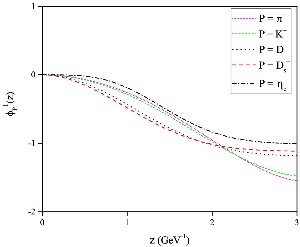
Now the wave functions for the studied mesons can be evaluated. The wave functions $\psi^{1}_{V}$ , $\psi^{1}_{A}$ , $\phi^{1}_{P}$ and $\pi^{1}_{P}$ as functions of $z$ are plotted in Fig. 3 for $\varepsilon\leq z\leq z_{0}$ . Here, $\rho^{-},a_{1}^{-}$ and $\pi^{-}$ are selected from the light mesons while, from the strange mesons we plot the wave functions for $K^{*-},K_{1A}^{-}$ and $K^{-}$ . Moreover, from the charm mesons group the plots are drawn for $D^{*-},D_{1}^{-}$ and $D^{-}$ states and the mesons $(D_{s}^{*-},D_{s1}^{-},D_{s}^{-})$ and ( $\psi,\chi_{{}_{c1}},\eta_{c}$ ) are chosen from the charmed-strange and $q\bar{q}$ states, respectively.

In this figure for the light, strange, charm, charm-strange and $q\bar{q}$ mesons, the plots are displaced with short-dot, short- dash, dot, dash and dash- dotted lines, respectively. For $(\pi^{-},\rho^{-},a_{1}^{-},K^{-},K^{*-},D^{-},D^{*-})$ the valuse of the masses, taken from the experimental data are reported in Table 2 while, for the other ground state mesons, the masses are taken form our predictions given in Table 3.

It should be noted that, since the values of $(m_{u},\sigma_{u})$ are close to those of $(m_{d},\sigma_{d})$ , and the masses of $D^{*0}$ and $D^{*-}$ have almost no differences, the plot of $\psi_{D^{*0}}$ is similar to the $\psi_{D^{*-}}$ . Similarities of plots of $\rho^{0}$ , $\pi^{0}$ , $D_{1}^{0}$ , $D^{0}$ and $K_{1A}^{0}$ are similar to those obtained for $\rho^{-}$ , $\pi^{-}$ , $D_{1}^{-}$ , $D^{-}$ and $K_{1A}^{-}$ , respectively. For this reason, in Fig. 3 just one of these two choices are displaced.

Now we move to 3-particle states couplings defined in Eqs. (49- 54). In this paper, to evaluate charm meson couplings to the axial vector mesons, the mass of $b_{1}^{-}$ is taken from PDG as $m_{b_{1}^{-}}=(1229.50\pm 3.20)~\rm{MeV}$ pdg. Moreover, for $K_{1B}^{-}$ , the mass is taken from 3PSR prediction as $m_{K_{1B}^{-}}=(1340\pm 80)~\rm{MeV}$ Kwei. Our predictions for $g_{{}_{D\,D\,A}}$ , $g_{{}_{D^{*}\,D\,A}}$ $g_{{}_{D\,D\,V}}$ , $g_{{}_{D^{*}\,D\,V}}$ , $g_{{}_{D^{*}\,D^{*}\,V}}$ and $g_{{}_{D_{1}\,D_{1}\,P}}$ are reported in Tables 5 and 6. Notice that the main uncertainty in the values of the couplings comes from $\sigma_{q},~(q=u,d,s,c)$ and the meson masses.

Table 5: Our predictions for the strong couplings of

(D,D,A)

and

(D^{*},D,A)

vertices.

$(D,D,A)$	$(D^{{}_{-}},\bar{D}^{{}_{0}},a_{1}^{{}_{-}})$	$(D^{{}_{-}},\bar{D}^{{}_{0}},b_{1}^{{}_{-}})$	$(D_{s}^{{}_{-}},\bar{D}^{{}_{0}},K_{1A}^{{}_{-}})$	$(D_{s}^{{}_{-}},\bar{D}^{{}_{0}},K_{1B}^{{}_{-}})$	$(D_{s}^{{}_{+}},{D}^{{}_{+}},K_{1A}^{{}_{0}})$	$(D_{s}^{{}_{+}},{D}^{{}_{+}},K_{1B}^{{}_{0}})$
$g_{{}_{D\,D\,A}}\,$	$0.32\pm 0.04$	$0.37\pm 0.04$	$0.89\pm 0.26$	$0.80\pm 0.21$	$0.92\pm 0.28$	$0.86\pm 0.17$
$(D^{*},D,A)$	$(D^{{}_{*-}},\bar{D}^{{}_{0}},a_{1}^{{}_{-}})$	$(D^{{}_{*}-},\bar{D}^{{}_{0}},b_{1}^{{}_{-}})$	$(D_{s}^{{}_{*}-},\bar{D}^{{}_{0}},K_{1A}^{{}_{-}})$	$(D_{s}^{{}_{*}-},\bar{D}^{{}_{0}},K_{1B}^{{}_{-}})$	$(D_{s}^{{}_{*}+},{D}^{{}_{+}},K_{1A}^{{}_{0}})$	$(D_{s}^{{}_{*}+},{D}^{{}_{+}},K_{1B}^{{}_{0}})$
$g_{{}_{D^{*}\,D\,A}}\,(\rm{GeV}^{-1})$	$1.94\pm 0.63$	$2.08\pm 0.52$	$2.27\pm 0.42$	$2.06\pm 0.35$	$2.47\pm 0.64$	$2.12\pm 0.36$

Table 6: Couplings for the

(D,D,V)

(D^{*},D,V)

(D^{*},D^{*}\,V)

and

(D_{1},D_{1},P)

vertices.

$(D,D,V)$	$(D^{{}_{-}},\bar{D}^{{}_{0}},\rho^{{}_{-}})$	$(D_{s}^{{}_{-}},\bar{D}^{{}_{0}},K^{{}_{*-}})$	$({D}^{{}_{0}},\bar{D}^{{}_{0}},\psi)$
$g_{{}_{D\,D\,V}}\,$	$1.02\pm 0.16$	$0.80\pm 0.06$	$3.03\pm 0.47$
$(D^{*},D,V)$	$(D^{{}_{*-}},\bar{D}^{{}_{0}},\rho^{{}_{-}})$	$(D_{s}^{{}_{-}},\bar{D}^{{}_{0}},K^{{}_{-}})$	$({D}^{{}_{*}0},\bar{D}^{{}_{0}},\psi$ )
$g_{{}_{D^{*}\,D\,V}}\,(\rm{GeV}^{-1})$	$1.29\pm 0.24$	$1.06\pm 0.10$	$5.02\pm 0.66$
$(D^{},D^{},V)$	$(D^{{}_{-}},\bar{D}^{{}_{0}},\rho^{{}_{-}})$	$(D_{s}^{{}_{-}},\bar{D}^{{}_{0}},K^{{}_{*-}})$	$({D}^{{}_{0}},\bar{D}^{{}_{0}},\psi)$
$g_{{}_{D^{}\,D^{}\,V}}$	$2.22\pm 0.27$	$1.78\pm 0.21$	$5.32\pm 0.70$
$(D_{1},D_{1},P)$	$(D_{1}^{{}_{-}},\bar{D}_{1}^{{}_{0}},\pi^{{}_{-}})$	$(D_{s1}^{{}_{-}},\bar{D}_{1}^{{}_{0}},K^{{}_{-}})$	$({D}_{1}^{{}_{0}},\bar{D}_{1}^{{}_{0}},\eta_{c})$
$g_{{}_{D_{1}\,D_{1}\,P}}\,(\rm{GeV}^{-1})$	$0.52\pm 0.11$	$0.83\pm 0.21$	$1.35\pm 0.29$

To evaluate strong couplings for $A=K_{1}(1270),K_{1}(1400)$ , the following relations are used:

$\displaystyle g_{D_{s}^{{}_{-}}\,\bar{D}^{{}_{0}}\,K_{1}(1270)^{{}_{-}}}$	$\displaystyle=$	$\displaystyle g_{D_{s}^{{}_{-}}\,\bar{D}^{{}_{0}}\,K_{1A}^{{}_{-}}}\,\sin\theta_{K}+g_{D_{s}^{{}_{-}}\,\bar{D}^{{}_{0}}\,K_{1B}^{{}_{-}}}\,\cos\theta_{K}\,,$	(76)
$\displaystyle g_{D_{s}^{{}_{-}}\,\bar{D}^{{}_{0}}\,K_{1}(1400)^{{}_{-}}}$	$\displaystyle=$	$\displaystyle g_{D_{s}^{{}_{-}}\,\bar{D}^{{}_{0}}\,K_{1A}^{{}_{-}}}\,\cos\theta_{K}-g_{D_{s}^{{}_{-}}\,\bar{D}^{{}_{0}}\,K_{1B}^{{}_{-}}}\,\sin\theta_{K}\,,$	(77)
$\displaystyle g_{D_{s}^{{}_{*-}}\,\bar{D}^{{}_{0}}\,K_{1}(1270)^{{}_{-}}}$	$\displaystyle=$	$\displaystyle r_{1A}\,g_{D_{s}^{{}_{-}}\,\bar{D}^{{}_{0}}\,K_{1A}^{{}_{-}}}\,\sin\theta_{K}+r_{1B}\,g_{D_{s}^{{}_{-}}\,\bar{D}^{{}_{0}}\,K_{1B}^{{}_{-}}}\,\cos\theta_{K}\,,$	(78)
$\displaystyle g_{D_{s}^{{}_{*-}}\,\bar{D}^{{}_{0}}\,K_{1}(1400)^{{}_{-}}}$	$\displaystyle=$	$\displaystyle r_{2A}\,g_{D_{s}^{{}_{-}}\,\bar{D}^{{}_{0}}\,K_{1A}^{{}_{-}}}\,\cos\theta_{K}-r_{2B}\,g_{D_{s}^{{}_{-}}\,\bar{D}^{{}_{0}}\,K_{1B}^{{}_{-}}}\,\sin\theta_{K}\,,$	(79)

where

	$\displaystyle r_{1A}=\frac{m^{2}_{D_{s}^{{}_{-}}}+m^{2}_{D_{0}}-m^{2}_{K_{1A}^{{}_{-}}}}{m^{2}_{D_{s}^{{}_{-}}}+m^{2}_{D_{0}}-m^{2}_{K_{1(1270)}^{{}_{-}}}},\,~~~~r_{1B}=\frac{m^{2}_{D_{s}^{{}_{-}}}+m^{2}_{D_{0}}-m^{2}_{K_{1B}^{{}_{-}}}}{m^{2}_{D_{s}^{{}_{-}}}+m^{2}_{D_{0}}-m^{2}_{K_{1(1270)}^{{}_{-}}}},\,$
	$\displaystyle r_{2A}=\frac{m^{2}_{D_{s}^{{}_{-}}}+m^{2}_{D_{0}}-m^{2}_{K_{1A}^{{}_{-}}}}{m^{2}_{D_{s}^{{}_{-}}}+m^{2}_{D_{0}}-m^{2}_{K_{1(1400)}^{{}_{-}}}},\,~~~~r_{2B}=\frac{m^{2}_{D_{s}^{{}_{-}}}+m^{2}_{D_{0}}-m^{2}_{K_{1B}^{{}_{-}}}}{m^{2}_{D_{s}^{{}_{-}}}+m^{2}_{D_{0}}-m^{2}_{K_{1(1400)}^{{}_{-}}}}.$		(80)

The $\theta_{K}$ dependence of the strong coupling constants $g_{D_{s}^{-}DK_{1}}$ and $g_{D_{s}^{*-}DK_{1}}$ for $K_{1}(1270)$ and $K_{1}(1400)$ are displaced in Fig. 4 with solid and dash lines, respectively. The uncertainty regions are also displayed in this figure.

Charm meson couplings to the vector, axial vector and the pseudoscalar mesons are evaluated via different approaches. Table 7, shows the values of the strong couplings calculated via LCSR momeni2020; Wanglscr2007 and 3PSR Bracco2010; Kim2001 as well as our predictions.

Table 7: The charm meson strong couplings in various theoretical approaches. Here,

g_{D^{{}_{*}}\,D\,A}

g_{D^{{}_{*}}\,D\,V}

and

g_{D_{1}\,D_{1}\,P}

are in the unit

\rm{GeV}^{-1}

Coupling constant	LCSR momeni2020	This work	Coupling constant	LCSR momeni2020	This work
$g_{D^{{}_{-}}\,\bar{D}^{{}_{0}}\,a_{1}^{{}_{-}}}$	$0.38\pm 0.07$	$0.32\pm 0.04$	$g_{D^{{}_{*-}}\,\bar{D}^{{}_{0}}\,a_{1}^{{}_{-}}}$	$1.03\pm 0.25$	$1.94\pm 0.63$
$g_{D^{{}_{-}}\,\bar{D}^{{}_{0}}\,b_{1}^{{}_{-}}}$	$1.64\pm 0.15$	$0.37\pm 0.04$	$g_{D^{{}_{*-}}\,\bar{D}^{{}_{0}}\,b_{1}^{{}_{-}}}$	$1.90\pm 0.72$	$2.08\pm 0.52$
$g_{D_{s}^{{}_{-}}\,\bar{D}^{{}_{0}}\,K_{1A}^{{}_{-}}}$	$1.17\pm 0.49$	$0.89\pm 0.26$	$g_{D_{s}^{{}_{*-}}\,\bar{D}^{{}_{0}}\,K_{1A}^{{}_{-}}}$	$1.36\pm 0.78$	$2.27\pm 0.42$
$g_{D_{s}^{{}_{-}}\,\bar{D}^{{}_{0}}\,K_{1B}^{{}_{-}}}$	$1.51\pm 0.11$	$0.80\pm 0.21$	$g_{D_{s}^{{}_{*-}}\,\bar{D}^{{}_{0}}\,K_{1B}^{{}_{-}}}$	$2.48\pm 0.78$	$2.06\pm 0.35$
Coupling constant	LCSR Wanglscr2007	This work	Coupling constant	LCSR Wanglscr2007	This work
$g_{D^{{}_{-}}\,\bar{D}^{{}_{0}}\,\rho^{{}_{-}}}$	$1.31\pm 0.29$	$1.02\pm 0.16$	$g_{D^{{}_{*-}}\,\bar{D}^{{}_{0}}\,\rho^{{}_{-}}}$	$0.89\pm 0.15$	$1.29\pm 0.24$
$g_{D_{s}^{{}_{-}},\bar{D}^{{}_{0}},K^{{}_{*-}}}$	$1.61\pm 0.32$	$0.80\pm 0.06$	$g_{D_{s}^{{}_{-}},\bar{D}^{{}_{0}},K^{{}_{-}}}$	$1.01\pm 0.20$	$1.06\pm 0.10$
Coupling constant	3PSR Bracco2010	This work	Coupling constant	3PSR Bracco2010; Kim2001	This work
$g_{{D}^{{}_{0}},\bar{D}^{{}_{0}},\psi}$	$5.80\pm 0.90$	$3.03\pm 0.47$	$g_{{D}^{{}_{*0}},\bar{D}^{{}_{0}},\psi}$	$4.00\pm 0.60$	$5.02\pm 0.66$
$g_{{D}^{{}_{0}},\bar{D}^{{}_{0}},\psi}$	$6.20\pm 0.90$	$5.32\pm 0.70$	$g_{D_{1}^{{}_{-}},\bar{D}_{1}^{{}_{0}},\pi^{{}_{-}}}$	$0.17\pm 0.04$	$0.52\pm 0.11$

Now, we consider the strong couplings for quadratic vertices. The values of $g_{\psi\,D^{(*)}\,D\,P}$ and $g_{\psi\,D^{(*)}\,D\,A}$ are listed in Tables 8 and 9. The reported values of $g_{{}_{\psi\,D^{*}\,D\,P}}$ are at $q^{2}=0$ . The strong couplings $g_{\psi\,D^{{}_{*0}}\,D^{{}_{+}}\,\pi^{{}_{-}}}$ , $g_{\psi\,D^{{}_{*0}}\,\bar{D}^{{}_{0}}\,\pi^{{}_{0}}}$ and $g_{\psi\,D_{s}^{{}_{*+}}\,D^{{}_{-}}\,K^{{}_{0}}}$ are plotted as functions of $q^{2}$ in Fig. 5. The values of $q^{2}_{\rm{max}}$ are $(m_{{D}^{{}_{+}}}+m_{\pi^{{}_{-}}})^{2}$ , $(m_{\bar{D}^{{}_{0}}}+m_{\pi^{{}_{0}}})^{2}$ and $(m_{D^{{}_{-}}}+m_{K^{{}_{0}}})^{2}$ for $(\psi,D^{{}_{*0}},D^{{}_{+}},\pi^{{}_{-}})$ , $(\psi,D^{{}_{*0}},\bar{D}^{{}_{0}},\pi^{{}_{0}})$ and $(\psi,D_{s}^{{}_{*+}},D^{{}_{-}},K^{{}_{0}})$ vertices, respectively.

Table 8: Our predictions for the couplings of

(\psi,D^{{}_{0(*0)}},D^{{}_{+}},\pi^{{}_{-}})

(\psi,D^{{}_{0(*0)}},\bar{D}^{{}_{0}},\pi^{{}_{0}})

and

(\psi,D_{s}^{{}_{+(*+)}},D^{{}_{-}},K^{{}_{0}})

vertices. The values of

(\psi,D^{*},D,P)

couplings are reported at

q^{2}=0

$(D,D,P)$	$(D^{{}_{0}},D^{{}_{+}},\pi^{{}_{-}})$	$(D^{{}_{0}},\bar{D}^{{}_{0}},\pi^{{}_{0}})$	$(D_{s}^{{}_{+}},D^{{}_{-}},K^{{}_{0}})$
$g_{{}_{\psi\,D\,D\,P}}\,~(\rm{GeV}^{-1})$	$1.28\pm 0.50$	$2.07\pm 0.85$	$0.49\pm 0.13$
$(D^{*},D,P)$	$(D^{{}_{*0}},D^{{}_{+}},\pi^{{}_{-}})$	$(D^{{}_{*0}},\bar{D}^{{}_{0}},\pi^{{}_{0}})$	$(D_{s}^{{}_{*+}},D^{{}_{-}},K^{{}_{0}})$
$g_{{}_{\psi\,D^{*}\,D\,P}}\,\,(q^{2}=0)$	$1.14\pm 0.08$	$1.05\pm 0.10$	$0.84\pm 0.04$

Table 9: Couplings for the

(D,D,V)

(D^{*},D,V)

(D^{*},D^{*}\,V)

and

(D_{1},D_{1},P)

vertices.

$(D,D,A)$	$(D^{{}_{0}},D^{{}_{+}},a_{1}^{{}_{-}})$	$(D^{{}_{0}},D^{{}_{+}},b_{1}^{-})$	$(D_{s}^{{}_{+}},D^{{}_{-}},K_{1A}^{{}_{0}})$	$(D_{s}^{{}_{+}},D^{{}_{-}},K_{1B}^{{}_{0}})$
$g_{{}_{\psi\,D\,D\,A}}\,$	$1.27\pm 0.03$	$1.30\pm 0.05$	$0.36\pm 0.10$	$0.38\pm 0.08$
$(D^{*},D,A)$	$(D^{{}_{*0}},D^{{}_{+}},a_{1}^{{}_{-}})$	$(D^{{}_{*0}},D^{{}_{+}},b_{1}^{-})$	$(D_{s}^{{}_{*+}},D^{{}_{-}},K_{1A}^{{}_{0}})$	$(D_{s}^{{}_{*+}},D^{{}_{-}},K_{1B}^{{}_{0}})$
$g_{{}_{\psi\,D^{*}\,D\,A}}\,\,~(\rm{GeV}^{-1})$	$0.12\pm 0.02$	$0.14\pm 0.02$	$0.50\pm 0.12$	$0.58\pm 0.11$

To evaluate the couplings of $(\psi,D_{s}^{{}_{+}},D^{{}_{-}},K_{1}^{{}_{0}}(1270))$ , $(\psi,D_{s}^{{}_{+}},D^{{}_{-}},K_{1}^{{}_{0}}(1400))$ , $(\psi,D_{s}^{{}_{*+}},D^{{}_{-}},K_{1}^{{}_{0}}(1270))$ and $(\psi,D_{s}^{{}_{*+}},D^{{}_{-}},K_{1}^{{}_{0}}(1400))$ vertices, we use the relations similar to those used in Eqs. (76) and (77). These couplings and their uncertainly regions are plotted as functions of the mixing angle $\theta_{K}$ in Fig 6. Our numeric analyze show that the main sources of uncertainties in the four particles vertices are $m_{c}$ and $\sigma_{c}$ .

In summary in this paper the two flavor hard-wall holographic model introduced in Erlich2005 is extended to four flavors. Our model consists of nine parameters including the hard wall position $z_{0}$ , quark masses $m_{q}$ and quark condensates $\sigma_{q}$ with $q=(u,d,s,c)$ . These parameters are fitted to the experimental masses of $\rho^{{}_{0}}$ , $\rho^{{}_{-}}$ , $a_{1}^{{}_{-}}$ , $\pi^{{}_{0}}$ , $\pi^{{}_{-}}$ $K^{{}_{-}}$ , $K^{{}_{*-}}$ , $D^{{}_{-}}$ and $D^{{}_{*-}}$ mesons. The masses and decay constants of some pseudoscalar, vector and axial vector mesons are evaluated using our model and a comparison is made between our predictions and the experimental data for these observables. After analyzing the wave functions, the strong couplings of $(D^{(*)},D,A)$ , $(D^{(*)},D^{(*)},V)$ , $(D_{1},D_{1},P)$ , $(\psi,D^{(*)},D,P)$ and $(\psi,D^{(*)},D,A)$ are analyzed. For $A=(K_{1}(1270),K_{1}(1400))$ the strong couplings are plotted as functions of the mixing angle $\theta_{K}$ . Moreover, for three mesons vertices a comparison is also made between our predictions and estimations made by other theoretical approaches.

Appendix A values for $g^{abc}$ , $h^{abc}$ , $l^{abc}$ , $k^{abc}$ , $h^{abcd}$ , $k^{abcd}$ and $l^{abcd}$

In this appendix, we present the nonzero values for $g^{abc}$ , $h^{abc}$ , $l^{abc}$ , $k^{abcd}$ , $h^{abcd}$ , $k^{abcd}$ and $l^{abcd}$ . The values results of the factors appeared in 3-point functions which are used in numerical analyze are given in Table 11.

Table 10: The values of

g^{abc}

h^{abc}

l^{abc}

and

k^{abc}

which are used in numerical analyze.

$(a,b,c)$	$g^{abc}$	$h^{abc}$	$l^{abc}$	$k^{abc}$
$(2,9,11)$	$\frac{1}{2}(v_{u}+v_{d})(v_{u}+v_{c})$	$\frac{1}{2}(v_{u}-v_{d})(v_{u}+v_{c})$	$\frac{1}{2}(v_{d}+v_{c})(v_{u}+v_{c})$	$\frac{1}{2}(v_{d}-v_{u})(v_{d}+v_{c})$
$(4,9,14)$	$\frac{1}{2}(v_{u}+v_{s})(v_{u}+v_{c})$	$\frac{1}{2}(v_{u}-v_{s})(v_{u}+v_{c})$	$\frac{1}{2}(v_{s}+v_{c})(v_{u}+v_{c})$	$\frac{1}{2}(v_{u}-v_{s})(v_{u}+v_{c})$
$(6,11,14)$	$-\frac{1}{2}(v_{d}+v_{s})(v_{s}+v_{c})$	$-\frac{1}{2}(v_{s}-v_{d})(v_{d}+v_{c})$	$\frac{1}{2}(v_{d}+v_{c})(v_{s}+v_{c})$	$-$
$(9,10,15)$	$\frac{\sqrt{6}}{6}(v_{u}+v_{c})(v_{u}+3\,v_{c})$	$\frac{\sqrt{6}}{6}(v_{u}-v_{c})(v_{u}-3\,v_{c})$	$-$	$\frac{\sqrt{6}}{6}(v_{d}-v_{c})(v_{d}+3\,v_{c})$

Table 11: The values of

g^{abcd}

h^{abcd}

l^{abcd}

and

k^{abcd}

which are used in numerical analyze.

$(a,b,c,d)$	$-i\,g^{abcd}$	$-i\,h^{abcd}$	$-i\,l^{abcd}$	$-i\,k^{abcd}$
$(9,15,2,11)$	$\frac{\sqrt{6}}{6}(v_{u}+v_{c})(v_{d}+v_{c})$	$-\frac{\sqrt{6}}{12}(v_{u}-v_{c})(v_{d}+v_{c})$	$-\frac{\sqrt{6}}{12}(v_{d}+v_{c})(v_{u}+3\,v_{c})$	$-\frac{\sqrt{6}}{12}(v_{u}+v_{d})(v_{u}+v_{c})$
$(9,15,3,10)$	$\frac{\sqrt{6}}{6}(v_{u}+v_{c})^{2}$	$-\frac{\sqrt{6}}{12}(v_{u}^{2}-v_{c}^{2})$	$-\frac{\sqrt{6}}{12}(v_{u}+v_{c})(v_{u}+3\,v_{c})$	$-\frac{\sqrt{6}}{6}v_{u}\,(v_{u}+v_{c})$
$(13,15,7,11)$	- $\frac{\sqrt{6}}{6}(v_{s}+v_{c})(v_{d}+v_{c})$	$\frac{\sqrt{6}}{12}(v_{d}+v_{c})(v_{s}-v_{c})$	$\frac{\sqrt{6}}{12}(v_{d}+v_{c})(v_{s}+3\,v_{c})$	$-\frac{\sqrt{6}}{12}(v_{d}+v_{c})(v_{s}+v_{c})$

References

(1) M. Janbazi, R. Khosravi, Eur. Phys. J. C 78, 606 (2018).
(2) M. Janbazi, R. Khosravi, E. Noori, Advances in High Energy Physics, 2018, 6045932 (2018).
(3) C. Isola, M. Ladisa, G. Nardulli, and P. Santorelli, Phys. Rev. D 68, 114001 (2003).
(4) C. Isola, M. Ladisa, G. Nardulli, T. N. Pham, and P. Santorelli, Phys. Rev. D 64, 014029 (2001).
(5) P. Colangelo, F. De Fazio and T.N. Pham, Phys.Rev. D 69, 054023 (2004).
(6) P. Colangelo, F. De Fazio and T.N. Pham, Phys. Lett. B 597, 291 (2004).
(7) M. Ladisa, V. Laporta, G. Nardulli and P. Santorelli, Phys.Rev. D70, 114025 (2004).
(8) H. Y. Cheng, C. K. Chua and A. Soni, Phys. Rev. D 71, 014030 (2005).
(9) A. Deandrea, M. Ladisa, V. Laporta, G. Nardulli and P. Santorelli, Int. J. Mod. Phys. A 21, 4425 (2006).
(10) M. E. Bracco, M. Chiapparini, F. S. Navarra and M. Nielson, Phys. Lett. B 605, 326 (2005).
(11) L.B. Holanda, R.S. Marques de Carvalho, A. Mihara, Phys. Lett. B 644, 232 (2007).
(12) K. U. Can, G. Erkol, M. Oka, A. Ozpineci and T. T. Takahashi, Phys. Lett. B 719, 103 (2013).
(13) A. Abada, D. Becirevic, Ph. Boucaud, G. Herdoiza, J.P. Leroy, A. Le Yaouanc, O. Pene and J. Rodríguez-Quintero, Phys. Rev. D 66, 074504 (2002).
(14) D. Becirevic and B. Haas, Eur. Phys. J. C 71, 1734 (2011).
(15) D. Becirevic and F. Sanfilippo, Phys. Lett. B 721, 94 (2013).
(16) M. E. Bracco, M. Chiapparini, F. S. Navarra, and M. Nielsen, Phys. Lett. B 659, 559 (2008).
(17) F. S. Navarra, M. Nielsen, M. E. Bracco, M. Chiapparini, and C. L. Schat, Phys. Lett. B 489, 319 (2000).
(18) F. S. Navarra, M. Nielsen, and M. E. Bracco, Phys. Rev. D 65, 037502 (2002).
(19) M. E. Bracco, M. Chiapparini, A. Lozea, F. S. Navarra, and M. Nielsen, Phys. Lett. B 521, 1 (2001).
(20) B. O. Rodrigues, M. E. Bracco, M. Nielsen, and F. S. Navarra, Nucl. Phys. A 852, 127 (2011).
(21) R. D. Matheus, F. S. Navarra, M. Nielsen, and R. R. da Silva, Phys. Lett. B 541, 265 (2002).
(22) R. R. da Silva, R. D. Matheus, F. S. Navarra, and M. Nielsen, Braz. J. Phys. 34, 236 (2004).
(23) Z. G. Wang, and S. L. Wan, Phys. Rev. D 74, 014017 (2006).
(24) Z. G. Wang, Nucl. Phys. A 796, 61 (2007).
(25) F. Carvalho, F. O. Duraes, F. S. Navarra, and M. Nielsen, Phys. Rev. C 72, 024902 (2005).
(26) M. E. Bracco, A. J. Cerqueira, M. Chiapparini, A. Lozea, and M. Nielsen, Phys. Lett. B 641, 286 (2006).
(27) L. B. Holanda, R. S. Marques de Carvalho, and A. Mihara, Phys. Lett. B 644, 232 (2007).
(28) R. Khosravi, and M. Janbazi, Phys. Rev. D 87, 016003 (2013).
(29) R. Khosravi1, and M. Janbazi, Phys. Rev. D 89, 016001 (2014).
(30) M. Janbazi, N. Ghahramany, and E. Pourjafarabadi, Eur. Phys. J. C 74, 2718 (2014).
(31) S. Momeni and R. Khosravi, arXiv: 2003.04165 [hep-ph].
(32) J. M. Maldacena, Adv. Theor. Math. Phys. 2, 231 (1998).
(33) E. Witten, Adv. Theor. Math. Phys. 2, 253 (1998), hep-
(34) S. S. Gubser, I. R. Klebanov, and A. M. Polyakov, Phys. Lett. B 428, 105 (1998).
(35) H. R. Grigoryan and A. V. Radyushkin, Phys. Lett. B 650, 421 (2007).
(36) Z. Abidin and C. E. Carlson, Phys. Rev. D 77, 095007 (2008).
(37) J. Polchinski and M. J. Strassler, Phys. Rev. Lett. 88, 031601 (2002).
(38) J. Polchinski and M. J. Strassler, JHEP 05, 012 (2003).
(39) S. J. Brodsky and G. F. de Teramond, Phys. Lett. B 582, 211 (2004).
(40) G. F. de Teramond and S. J. Brodsky, Phys. Rev. Lett. 94, 201601 (2005).
(41) S. J. Brodsky and G. F. de Teramond, Phys. Rev. Lett. 96, 201601 (2006).
(42) S. J. Brodsky and G. F. de Teramond, Phys. Rev. D 78, 025032 (2008).
(43) H. R. Grigoryan and A. V. Radyushkin, Phys. Rev. D 76, 095007 (2007).
(44) H. R. Grigoryan and A. V. Radyushkin, Phys. Rev. D 76, 115007 (2007).
(45) H. R. Grigoryan and A. V. Radyushkin, Phys. Rev. D 78, 115008 (2008).
(46) H. J. Kwee and R. F. Lebed, JHEP 01, 027 (2008).
(47) H. J. Kwee and R. F. Lebed, Phys. Rev. D 77, 115007 (2008).
(48) H. Boschi-Filho, N. R. F. Braga, and H. L. Carrion, Phys. Rev. D 73, 047901 (2006).
(49) Z. Abidin and C. E. Carlson, Phys. Rev. D 78, 071502
(50) Z. Abidin and C. E. Carlson, Phys. Rev. D 79, 115003 (2009).
(51) Z. Abidin and C. E. Carlson, Phys. Rev. D 80, 115010 (2009).
(52) A. B. Bayona, G. Krein and C. Miller, Phys. Rev. D 96, 014017 (2017).
(53) J. Erlich, E. Katz, D. T. Son, and M. A. Stephanov, Phys. Rev. Lett. 95, 261602 (2005).
(54) J. P. Shock and F. Wu, JHEP 08, 023 (2006).
(55) E. Katz and M. D. Schwartz, JHEP 08, 077 (2007).
(56) A. Cherman, T. D. Cohen and E. S. Werbos, Phys. Rev. C 79, 045203 (2009).
(57) P. Colangelo, F. De Fazio, F. Giannuzzi, F. Jugeau, S. Nicotri, Phys. Rev. D 78, 055009 (2008).
(58) N. Maru, M. Tachibana, Eur. Phys. J. C 63, 123-132 (2009).
(59) N. Huseynova, S. Mamedov, arXiv: 1907.13477 [hep-ph].
(60) L. Burakovsky and T. Goldman, Phys. Rev. D 57, 2879 (1998).
(61) M. Suzuki, Phys. Rev. D 47, 1252 (1993).
(62) T. M. Aliev and N. K. Pak, M. Savci, Phys. Lett. B 390 335-340 (1997).
(63) V. M. Belyaev, V. M. Braun, A. Khodjamirian and R. Ruckl, Phys. Rev. D 51, 6177 (1995).
(64) M.E. Bracco, M. Chiapparini, F.S. Navarra, M. Nielsen, Prog. Part. Nucl. Phys. 67, 1019 (2012).
(65) M. A. A. Sbaih, M. K. H. Srour, M. S. Hamada and H. M. Fayad, , Electronic Journal of Theoretical Physics. 28, 9 (2013).
(66) Z. Abidin and C. E. Carlson, Phys. Rev. D 77, 115021 (2008).
(67) M. Tanabashi et al. (Particle Data Group), Phys. Rev. D 98, 030001 (2018).
(68) Particle Data Group, C. Amsler et al., Phys. Lett. B 667, 1 (2008).
(69) K. Yang, Nucl. Phys. B 776, 187 (2007).
(70) J. F. Donoghue, E. Golowich and B. R. Holstein, Dynamics of the standard model (Cambridge, New York, 2014).
(71) N. Isgur, C. Morningstar and C. Reader, Phys. Rev. D 39, 1357 (1989).
(72) Z. G. Wang, Nucl. Phys. A 796, 61-82 (2007).
(73) M. E. Bracco, M. Chiapparini, F. S. Navarra and M. Nielsen, Prog. Part. Nucl. Phys. 67, 1019 (2012).
(74) H. Kim, S. H. Lee, Eur. Phys. J. C 22, 707-713 (2002).

$\displaystyle\langle D(p_{1})\|A(p_{2},\varepsilon^{\prime})\,D(p_{3})\rangle$	$\displaystyle=$	$\displaystyle 2\,(\varepsilon^{\prime}.p_{3})\,g_{{}_{DDA}},$
$\displaystyle\langle D^{*}(p_{1},\varepsilon)\|A(p_{2},\varepsilon^{\prime})\,D(p_{3})\rangle$	$\displaystyle=$	$\displaystyle\big[(\varepsilon^{}.\varepsilon^{\prime})\,(p_{3}.p_{1})-(\varepsilon^{}.p_{3})\,(\varepsilon^{\prime}.p_{1})\big.]\,g_{{}_{D^{*}\,D\,A}},$
$\displaystyle\langle D(p_{1})\|V(p_{2},\varepsilon)\,D(p_{3})\rangle$	$\displaystyle=$	$\displaystyle 2\,(\varepsilon.p_{3})g_{{}_{DDV}},$
$\displaystyle\langle D^{*}(p_{1},\varepsilon_{1})\|V(p_{2},\varepsilon_{2})\,D(p_{3})\rangle$	$\displaystyle=$	$\displaystyle\big[(\varepsilon_{1}^{}.\varepsilon_{2})\,(p_{3}.p_{1})-(\varepsilon_{1}^{}.p_{3})\,(\varepsilon_{2}.p_{1})\big]\,g_{{}_{D^{*}\,D\,V}},$
$\displaystyle\langle D^{}(p_{1},\varepsilon_{1})\|V(p_{2},\varepsilon_{2})\,D^{}(p_{3},\varepsilon_{3})\rangle$	$\displaystyle=$	$\displaystyle(\varepsilon^{}_{1}.\varepsilon_{2})\,(\varepsilon_{3}.p_{3})\,g_{{}_{D^{}\,D^{*}\,V}},$
$\displaystyle\langle D_{1}(p_{1},\varepsilon^{\prime}_{1})\|P(p_{2})\,D_{1}(p_{3},\varepsilon^{\prime}_{2})\rangle$	$\displaystyle=$	$\displaystyle\big[(\varepsilon_{1}^{{}^{\prime}}.\varepsilon_{2}^{{}^{\prime}})\,(p_{3}.p_{1})-(\varepsilon_{1}^{{}^{\prime}}.p_{3})\,(\varepsilon^{\prime}_{2}.p_{1})\big]\,g_{{}_{D_{1}\,D_{1}\,P}},$	(29)

	$\displaystyle\langle D(p_{1})\|A(p_{2},\varepsilon^{\prime})\,D(p_{3})\rangle=\Omega_{\alpha\beta}(1,3)\,\Lambda(D\,A\,D)\,\varepsilon^{\prime}_{\mu}\,\hat{\mathcal{L}}\Bigg(\langle 0\|\mathcal{T}\left.\{J_{A\parallel}^{\alpha a}(x)J_{A\perp}^{\mu b}(0)J_{A\parallel}^{\beta c}(w)\right.\}\|0\rangle\Bigg),$

	$\displaystyle\langle D^{}(p_{1},\varepsilon)\|A(p_{2},\varepsilon^{\prime})\,D(p_{3})\rangle=\Omega_{\alpha}(3)\,\Lambda(D^{}\,A\,D)\,\,\varepsilon^{*}_{\mu}\,\varepsilon^{\prime}_{\nu}\,\hat{\mathcal{L}}\Bigg(\langle 0\|\mathcal{T}\left.\{J_{V\perp}^{\mu a}(x)J_{A\perp}^{\nu b}(0)J_{A\parallel}^{\alpha c}(w)\right.\}\|0\rangle\Bigg),$

	$\displaystyle\langle D(p_{1})\|V(p_{2},\varepsilon)\,D(p_{3})\rangle=\Omega_{\alpha\beta}(1,3)\,\Lambda(D\,V\,D)\,\varepsilon_{\mu}\,\hat{\mathcal{L}}\Bigg(\langle 0\|\mathcal{T}\left.\{J_{A\parallel}^{\alpha a}(x)J_{V\perp}^{\mu b}(0)J_{A\parallel}^{\beta c}(w)\right.\}\|0\rangle\Bigg),\,$

	$\displaystyle\langle D^{}(p_{1},\varepsilon_{1})\|V(p_{2},\varepsilon_{2})\,D(p_{3})\rangle=\Omega_{\alpha}(3)\,\Lambda(D^{}\,V\,D)\,\varepsilon^{*}_{1\mu}\,\varepsilon_{2\nu}\,\hat{\mathcal{L}}\Bigg(\langle 0\|\mathcal{T}\left.\{J_{V\perp}^{\mu a}(x)J_{V\perp}^{\nu b}(0)J_{A\parallel}^{\alpha c}(w)\right.\}\|0\rangle\Bigg),$

	$\displaystyle\langle D^{}(p_{1},\varepsilon_{1})\|V(p_{2},\varepsilon_{2})\,D^{}(p_{3},\varepsilon_{3})\rangle=\Lambda(D^{}\,V\,D^{})\,\varepsilon^{*}_{1\mu}\,\varepsilon_{2\nu}\,\varepsilon_{3\sigma}\hat{\mathcal{L}}\Bigg(\langle 0\|\mathcal{T}\left.\{J_{V\perp}^{\mu a}(x)J_{V\perp}^{\nu b}(0)J_{V\perp}^{\sigma c}(w)\right.\}\|0\rangle\Bigg),$

	$\displaystyle\langle D_{1}(p_{1},\varepsilon^{\prime}_{1})\|P(p_{2})\,D_{1}(p_{3},\varepsilon^{\prime}_{2})\rangle=\Omega_{\alpha}(2)\,\Lambda(D_{1}\,P\,D_{1})\,\,\varepsilon^{{}^{\prime}*}_{1\mu}\,\varepsilon^{\prime}_{2\nu}\,\hat{\mathcal{L}}\Bigg(\langle 0\|\mathcal{T}\left.\{J_{A\perp}^{\mu a}(x)J_{A\perp}^{\nu b}(0)J_{A\parallel}^{\alpha c}(w)\right.\}\|0\rangle\Bigg),$

	$\displaystyle\langle\psi(p_{1},\varepsilon)\|D(p_{2})D(p_{3})\,P(p_{4})\rangle=\Omega_{\alpha\beta\delta}(2,3,4)\,\Lambda(\psi\,D\,D\,P)\,\varepsilon^{*}_{\mu}\,\hat{\hat{\mathcal{L}}}\Bigg(\langle 0\|\mathcal{T}\left.\{J_{V\perp}^{\mu a}(x)J_{A\parallel}^{\alpha b}(y)\,J_{A\parallel}^{\beta c}(0)J_{A\parallel}^{\delta d}(u)\right.\}\|0\rangle\Bigg),$

	$\displaystyle\langle\psi(p_{1},\varepsilon)\|D(p_{2})D(p_{3})\,A(p_{4},\varepsilon^{\prime})\rangle=\Omega_{\alpha\beta}(2,3)\Lambda(\psi\,D\,D\,A)\,\varepsilon^{*}_{\mu}\,\varepsilon^{\prime}_{\nu}\hat{\hat{\mathcal{L}}}\Bigg(\langle 0\|\mathcal{T}\left.\{J_{V\perp}^{\mu a}(x)J_{A\parallel}^{\alpha b}(y)\,J_{A\parallel}^{\beta c}(0)J_{A\perp}^{\nu d}(u)\right.\}\|0\rangle\Bigg),$

	$\displaystyle\langle\psi(p_{1},\varepsilon_{1})\|D^{}(p_{2},\varepsilon_{2})D(p_{3})\,P(p_{4})\rangle=\Omega_{\alpha\beta}(3,4)\,\Lambda(\psi\,D^{}\,D\,P)\,\varepsilon^{*}_{1\mu}\,\varepsilon_{2\nu}\hat{\hat{\mathcal{L}}}\Bigg(\langle 0\|\mathcal{T}\left.\{J_{V\perp}^{\mu a}(x)J_{V\perp}^{\nu b}(y)\,J_{A\parallel}^{\alpha c}(0)J_{A\parallel}^{\beta d}(u)\right.\}\|0\rangle\Bigg),$

	$\displaystyle\langle\psi(p_{1},\varepsilon_{1})\|D^{}(p_{2},\varepsilon_{2})D(p_{3})\,A(p_{4},\varepsilon^{\prime})\rangle=\Omega_{\alpha}(3)\,\Lambda(\psi\,D^{}\,D\,A)\,\varepsilon^{*}_{1\mu}\,\varepsilon_{2\nu}\,\varepsilon^{\prime}_{\sigma}\hat{\hat{\mathcal{L}}}\Bigg(\langle 0\|\mathcal{T}\left.\{J_{V\perp}^{\mu a}(x)J_{V\perp}^{\nu b}(y)\,J_{A\parallel}^{\alpha c}(0)J_{A\perp}^{\sigma d}(u)\right.\}\|0\rangle\Bigg),$

Charm meson couplings in hard-wall Holographic QCD

Abstract

pacs

I Introduction

II The AdS/QCD model involving pseudoscalar, vector and axial vector mesons

III Wave functions, masses and the decay constants for the pseudoscalar, vector and axial vector mesons

III.1 Wave functions

III.2 Decay constants

IV Strong coupling constants from three and four point functions

IV.1 3-point functions and charm meson couplings

IV.2 4-point functions and charm meson couplings

V Numerical analysis

Appendix A values for ga​b​cg^{abc}, ha​b​ch^{abc}, la​b​cl^{abc}, ka​b​ck^{abc}, ha​b​c​dh^{abcd}, ka​b​c​dk^{abcd} and la​b​c​dl^{abcd}

References

Appendix A values for $g^{abc}$ , $h^{abc}$ , $l^{abc}$ , $k^{abc}$ , $h^{abcd}$ , $k^{abcd}$ and $l^{abcd}$