Geographically Weighted Regression Analysis for Spatial Economics Data: a Bayesian Recourse
Abstract
The geographically weighted regression (GWR) is a well-known statistical approach to explore spatial non-stationarity of the regression relationship in spatial data analysis. In this paper, we discuss a Bayesian recourse of GWR. Bayesian variable selection based on spike-and-slab prior, bandwidth selection based on range prior, and model assessment using a modified deviance information criterion and a modified logarithm of pseudo-marginal likelihood are fully discussed in this paper. Usage of the graph distance in modeling areal data is also introduced. Extensive simulation studies are carried out to examine the empirical performance of the proposed methods with both small and large number of location scenarios, and comparison with the classical frequentist GWR is made. The performance of variable selection and estimation of the proposed methodology under different circumstances are satisfactory. We further apply the proposed methodology in analysis of a province-level macroeconomic data of 30 selected provinces in China. The estimation and variable selection results reveal insights about China’s economy that are convincing and agree with previous studies and facts.
Keywords: MCMC, Model Assessment, Spatial Econometrics, Variable Selection
Introduction
For geographically sparse data with inherent spatial variability, estimating coefficients of a regression model for a particular location based on only observations from this location is not feasible due to the small number of observations. The geographically weighted regression (Brunsdon et al. 1996, GWR;) is an important tool to explore spatial non-stationarity of the regression relationship in spatial data analysis. It has been applied to a variety of fields, including geology, environmental science, epidemiology, and econometrics. Fotheringham et al. 2002 has summarized the basic theory, statistical inference, and bandwidth selection for GWR, and proposed natural extensions of GWR under the generalized linear model framework. The basic idea of GWR is to make use of information from nearby locations. The weighting idea is a natural strategy to use in light of Tobler’s first law that “near things are more related than distant things” (Tobler 1970). In estimating the parameter for one specific location, subjects in the data are weighed according to their distance from this location, with greater weight for closer subjects. Páez et al. 2002a; Páez et al. 2002b proposed estimation and inference for GWR under a maximum-likelihood-based framework. Mei et al. 2006 proposed a mixed geographically weighted regression model which included both spatially-varying and non-spatially-varying coefficients, and gave a testing procedure of important explanatory variables. Wang et al. 2008 proposed a local linear-based GWR for the spatially varying coefficient models which can significantly improve GWR. More recently, da Silva and Fotheringham 2016 discussed the multiple testing issue, and proposed a solution which outperforms other solutions such as the Bonferroni procedure under the GWR framework. The aforementioned works discussed the GWR in the frequentist fashion. From the Bayesian perspective, LeSage 2004 proposed a Bayesian GWR, which gives a prior distribution on the parameter vector depending on historical knowledge. The proposed model, however, used cross-validation for bandwidth selection, which relies on a user-specified grid of bandwidth, and is computationally intensive like other cross-validation based methods.
In this paper, we propose Bayesian techniques for the GWR using the likelihood-based approach in Páez et al. 2002a; Páez et al. 2002b. In addition to Bayesian estimation and inference, a spike and slab (Ishwaran et al. 2005) prior is applied for variable selection for Bayesian GWR. Furthermore, bandwidth selection and weighting scheme selection are discussed based on prior selection and Bayesian model selection criteria. An introduction to the implementation of GWR based on nimble (de Valpine et al. 2017), a relatively new and powerful R package for Bayesian inference, is presented as an open source repository on GitHub. Our simulation studies showed the promising empirical performance of the proposed methods in both non-spatially varying and spatially varying cases. In addition, our proposed Bayesian approach reveals interesting features of the province-level macroeconomic data in China.
The rest of this paper is organized as follows. In Section “Geographically Weighted Regression”, the GWR and its weighting schemes are discussed. Section “Bayesian Recourse for GWR” gives a detailed discussion of Bayesian inference, variable selection, bandwidth selection, and model assessment for the GWR. Extensive simulation studies are conducted in Section “Simulation Studies” to investigate the empirical performance of the proposed methods. In Section “Real Data Analysis”, we implement our model using province-level macroeconomic data in China from year 2012 to year 2016. Finally, Section “Discussion” contains a brief summary of this paper.
Geographically Weighted Regression
Geographically Weighted Regression
From Brunsdon et al. 1998 , the GWR model can be written as:
| (1) |
where is the response variable at location , , are the coefficients of independent variables at location , and is the random effect at location , assumed to follow . In addition, we also assume for any . Given a weighting function, the weights of each observation can be calculated with the distance between that observation and . Estimation of coefficients at location can be formulated in a way similar to the weighted least squares:
| (2) |
where is the matrix of covariates, is the vector of responses, and is a diagonal matrix of the weights.
Spatial Weighting Functions and Distances
We first introduce several spatial weighting functions that can be used in GWR. Notice that the weighting scheme of ordinary least squares can be defined in the following form:
| (3) |
where represents the location of the observations, and represents the location for which parameters are estimated. In a global model where observations from all locations are used to estimate one vector of coefficients, each observation is assigned a weight of unity.
A first step to consider locality is to include observations that are only within a certain distance from the target location, i.e.,
| (4) |
where is the distance between locations and . This weighting scheme is one of the simplest to calculate. It is, however, a discontinuous function of distance, which can sometimes lead to undesired jumps in the estimated parameter surface. In order to get a continuous weighting function, the exponential function and the Gaussian function can also be used. The exponential weighting scheme can be written as:
| (5) |
where is the bandwidth that can be chosen appropriately to control the decay with respect to distance. The Gaussian weighting scheme can be written as:
| (6) |
Both (5) and (6) are decreasing functions of , which, intuitively, indicates that an observation very far away from the location of interest contributes little in the estimation of parameters at this location. In order to provide a continuous, near-Gaussian weighting function up to distance from the estimation point, and then zero weights for any data point beyond , Brunsdon et al. 1996; Brunsdon et al. 1998; Fotheringham et al. 1998 proposed the bi-square function:
| (7) |
For the bi-square kernel, by tuning the threshold , one can control the number of neighbors that are used to estimate the parameters for the location of interest. The weighting schemes mentioned above are the most popular schemes used in the GWR.
We then briefly discuss different choices of distance function. The Euclidean distance, defined as
is one of the most popular choices when the precise (latitude, longitude) location of each observation is available. However, in some public health and epidemiology studies, or some socioeconomics studies, data are collected and summarized on a higher level than single observations, such as wards (Brunsdon et al. 1996) or counties (Xue et al. 2019), which produces areal data instead of point-reference data. All observations within the same area are assigned the same (latitude, longitude). For example, Hu and Huffer 2020 attributed each county’s observations to its centroid. Note that the Euclidean distance is easily affected by the areas of the administrative divisions, which additionally complicates the process of parameter tuning as there is no golden benchmark measure of distance.
An alternative distance measure when we have areal data is the graph distance (Müller et al. 1987; Bhattacharyya and Bickel 2014). The administrative devisions are regarded as vertices of a graph , denoted as . The graph also includes a set of edges, , where each edge connects a pair of vertices. The graph distance is defined as:
| (8) |
where denotes the number of edges in .
While it remains a subjective problem in choosing appropriate bandwidths and thresholds for the geographical distance based methods, i.e. one has to decide “how close is close enough”, a natural definition of closeness would derive from the graph distance. Counties sharing a common boundary, i.e. having graph distance 1, are close, while having graph distance greater than 1 indicates “not close”, and observations in these far neighboring counties need to be weighed down. A graph distance based weighting function would be
| (9) |
where denotes the graph distance, and is a certain weighting function with bandwidth . In this work, we choose to be the negative exponential function, i.e.,
| (10) |
Bayesian Recourse for GWR
In this section, we propose the posterior estimation, variable selection, and bandwidth selection for the Bayesian GWR model. The proposed methods are implemented with the powerful R package nimble. The code and documentation can be found at GitHub.
Bayesian Estimation for GWR
According to Boscardin and Gelman 1993 and Páez et al. 2002a; Páez et al. 2002b, we can get the estimation of GWR using Bayesian computation. The likelihood function of this model can be written as:
| (11) |
where MVN indicates the multivariate normal distribution. In order to have a conjugate posterior distribution, we can set the priors of and as:
| (12) |
where is a diagonal matrix, and
| (13) |
where are the hyper-parameters for distributions of . One set of non-informative choices of hyper-parameters is to set and (Gelman et al. 2013). The posterior distribution can be written as:
| (14) |
According to (14), we can use Markov chain Monte Carlo (Gelman et al. 2013, MCMC,) to estimate and .
Bayesian Variable Selection
We first consider the regression problem for one location. Following the procedure of George and McCulloch 1993, the spike and slab prior for can be formulated as:
| (15) |
where
| (16) |
When , , and when , . Our interpretation of this prior is: we set small enough so that if , would be so small that we can “safely” estimate it as 0; inversely, we set large so that if , we include the into our final model. For the prior of , we set , which is a non-informative choice.
Bayesian Bandwidth Selection
In GWR, it is important to choose a proper bandwidth for the weighting functions. In the Bayesian approach, a prior can be given to the bandwidth so that the optimal bandwidth can be simultaneously obtained together with the estimation of other parameters. The prior also depends on which measure of distance is used. A more detailed discussion of distance measures is given in Section “Spatial Weighting Function and Distances”. Using similar ideas as in Boehm Vock et al. 2015, a prior for bandwidth can be set as:
where is the upper limit for the support of the distribution of . Without any prior knowledge, can be chosen large enough so that we start from a noninformative prior for the bandwidth, i.e., we start from an approximate global model where observations are always weighed equally. There are also some other choices of prior distributions for the bandwidth, such as the gamma distribution or discrete uniform distribution. If prior information is available about the bandwidth, parameters for the prior distributions can be set to incorporate such information. Our proposed model can be summarized as follows:
| (17) | |||
| (18) | |||
| (19) | |||
| (20) | |||
| (21) | |||
| (22) |
where “IGamma” denotes the inverse-Gamma distribution, and is the weighting function introduced in (9), and . As we incorporate the prior of into our model, conjugate posterior distribution for cannot be obtained. Therefore, we use the Metropolis–Hastings Algorithm (Gelman et al. 2013, MH;) to estimate the parameters.
Bayesian Model Assesment
In Section “Spatial Weighting Function and Distances”, we introduced several spatial weighting functions that can be used in the GWR. In order to select the weighting scheme that fits the data best, we apply the most commonly used tools, the Deviance Information Criterion (Spiegelhalter et al. 2002, DIC;) and the Logarithm of the Pseudo-Marginal Likelihood (Ibrahim et al. 2013, LPML;), for model selection. The DIC is defined as:
| (23) |
where and represent the parameter of interest and the corresponding posterior mean. The term denotes the deviance function, while is the effective number of parameters in the model, given by . For the GWR model in our paper, the following deviance function can be specified (Ma et al. 2018):
where is the total number of the observations. Therefore, the DIC for the GWR model can be given as:
| DIC | |||
where , and are posterior estimates obtained from MCMC results. A smaller value of DIC indicates a better model. It can be regarded as the Bayesian equivalent of AIC, where the term is the penalty term for model complexity, similar to the , i.e., dimension of parameter space, in AIC. Similar to AIC, DIC also takes both fitness and model complexity into account simultaneously.
The LPML is constructed based on the Conditional Predictive Ordinate (CPO) values, which are estimates of the probability for observing given that all other responses have been observed. Let denote the observed data with the th subject response deleted. The CPO for the th subject is defined as:
| (24) |
where , and denotes the normalizing constant. Within the Bayesian framework, a Monte Carlo estimate of the CPO can be obtained as:
where is the total number of Monte Carlo iterations. Then an estimate of the LPML is given by:
| (25) |
A model with a larger LPML value indicates that it is more preferred.
Simulation Studies
In this section, we present the performance of the proposed estimation and variable selection techniques under scenarios where the covariate effects do not vary spatially, and where the covariate effects do vary spatially. We use the spatial structure of 30 selected provinces in China in our simulations. A map of these provinces with their names is presented in Figure 1(a). Specifically, Hainan province is an island, and is therefore not connected with any others, which makes its graph distance with any other province infinity. It is, however, very close to Guangdong province, and they bear a lot of resemblance in both culture and economic development. Therefore, we modified the adjacency matrix so that Hainan and Guangdong are adjacent. The graph distance matrix is calculated based on the modified adjacency matrix. A visualization of the graph distance matrix is presented in Figure 1(b).


Denote the average parameter estimates as , calculated as
| (26) |
where denotes the parameter estimate for the th coefficient of province in the th replicate. The parameter estimates are evaluated based on their bias, standard deviation, mean squared error, and coverage rate of the 95% highest posterior density (HPD) intervals in the following four ways:
| mean absolute bias (MAB) | (27) | |||
| mean standard deviation (MSD) | (28) | |||
| mean of mean squared error (MMSE) | (29) | |||
| mean coverage rate (MCR) | (30) |
where is the true underlying parameter, and denotes the indicator function. These measures are first calculated for each individual province over replicates, and then averaged over provinces. The variable selection approach is evaluated using both the accuracy rate for a single variable ACC and for the entire model (Model ACC), defined as:
and
To compare with frequentist approach, the same datasets are also fitted using the classical frequentist GWR approach, where the bandwidth selection is made based on minimizing the summation of SSE across 30 provinces over a grid of candidate bandwidths. The details of frequentist bandwdith selection, as well as the parameter estimates obtained using the optimal bandwdith, are presented in Section 1 of the supplemental material. To demonstrate that the graph distance produces credible parameter estimates, and that at the same time it circumvents the additional effort of threshold selection in weighting kernels such as (4) and (10), simulation study is done for the same designs to be presented, with the great circle distance used. The results are reported in Section 2 of the supplemental material. In addition, considering that a total of 150 observations with 30 locations still make a small sample, an additional simulation study with more than 300 locations using the spatial structure of census tracts in Hartford, Litchfield, and Middletown counties in Connecticut has been conducted, and included in Section 3 of the supplemental material.
For both the following simulation studies and the supplemental simulation studies, the effective number of parameters for the frequentist GWR is also calculated as in Brunsdon et al. 2000. Note that the frequentist GWR is based on one bandwidth only, and only the full model that includes all covariates is fitted, therefore the frequentist should be used as a reference, instead of a criteria for direct comparison.
Simulation Without Spatially Varying Coefficients
Under the scenario where there are no spatially varying coefficients, we generate data using the same set of parameters for all provinces. The independent continuous covariates are generated i.i.d. from the standard normal distribution , denoted as , ,…, , and we use the matrix to denote the covariate matrix with 5 columns, with the th column being . The response vector is generated as , where . Different choices of have been used corresponding to different underlying true models. The parameter for bandwidth is set to be 100. Given that the maximum graph distance in the spatial structure of the 30 selected provinces is 6, a bandwidth of 100 induces a weighting schemes that, even if the distance between one certain province and another province whose parameter estimates we want to obtain, this province gets assigned a relative weight of , which is approximately 0.941 and thus approximates a global model where every observation is equally weighed. This ensures that the prior for bandwidth is sufficiently noninformative. For each province, five observations are generated, resulting in 150 observations per replicate. A total of 100 replicates are performed. For each replicate, a chain of length 10,000 is run without thinning, where the first 2,000 samples are discarded as burn-in. Three parameter settings similar to in Shao 1997 were used, with , , and , respectively. The mean of bandwidths selected in the 100 replicates was also calculated. The results are reported in Table 1.
It is rather clear that when there is no spatial variation, the bandwidth is selected to be large, which induces a weighting scheme that assigns close to uniform weight to both nearby provinces and distant provinces. Under all three settings, the variable selection accuracies are all 100% for all five covariates, and the three model selection accuracies are 100% as well. The average effective number of parameters under the frequentist GWR are 11.08, 10.27 and 12.65 under the three settings, while under the Bayesian GWR, the values are 178.00, 177.89 and 177.57, respectively.
| MAB | MSD | MMSE | MCR | True | ACC(%) | Model ACC(%) | ||||
|---|---|---|---|---|---|---|---|---|---|---|
| Setting 1 | 1.998 | 0.055 | 0.074 | 0.005 | 0.942 | 1 | 100 | 100 | 70.112 | |
| 0.007 | 0.037 | 0.046 | 0.002 | 0.990 | 0 | 100 | ||||
| 0.004 | 0.040 | 0.049 | 0.002 | 0.999 | 0 | 100 | ||||
| 4.019 | 0.062 | 0.077 | 0.006 | 0.974 | 1 | 100 | ||||
| 7.990 | 0.066 | 0.085 | 0.007 | 0.934 | 1 | 100 | ||||
| Setting 2 | 1.998 | 0.055 | 0.073 | 0.005 | 0.942 | 1 | 100 | 100 | 70.213 | |
| 2.012 | 0.064 | 0.080 | 0.006 | 0.975 | 1 | 100 | ||||
| 0.003 | 0.040 | 0.049 | 0.002 | 1.000 | 0 | 100 | ||||
| 4.019 | 0.062 | 0.077 | 0.006 | 0.975 | 1 | 100 | ||||
| 7.991 | 0.066 | 0.085 | 0.007 | 0.934 | 1 | 100 | ||||
| Setting 3 | 1.997 | 0.055 | 0.073 | 0.005 | 0.939 | 1 | 100 | 100 | 70.058 | |
| 2.012 | 0.065 | 0.080 | 0.007 | 0.973 | 1 | 100 | ||||
| 3.005 | 0.068 | 0.084 | 0.007 | 0.954 | 1 | 100 | ||||
| 4.018 | 0.062 | 0.076 | 0.006 | 0.977 | 1 | 100 | ||||
| 7.990 | 0.067 | 0.085 | 0.007 | 0.936 | 1 | 100 |
Simulation with Spatially Varying Coefficients
For estimation and variable selection in the presence of spatially varying coefficients, we use similar simulation schemes as in Xue et al. 2019. The graph distance matrix visualized in Figure 1 is transformed using multidimensional scaling (Cox and Cox 2000, MDS;) and mapped into a Cartesian space. Denoting the transformed coordinates corresponding to province as , the vector for province is set to
| (31) |
The variation pattern is visualized in Figure 2. The estimation and variable selection results for the setting in (31) are presented in Table 2. It can be seen that in all three settings, the MAB, MSD and MMSE are all larger than when there is no spatially varying covariate effects. There have been decrease in the MCR for parameters corresponding to covariates that are in the true model. The variable selection procedure, however, remains quite robust, and in all replicates of simulation are the correct models selected. The average bandwidths selected for the three settings are around 67. This indicates that in the presence of spatial variation, for some replicates of simulation, the bandwidths tend to be large as the gain in stabilizing the parameter estimates for each location dominates the incurred bias. This has also been observed for the classical frequentist GWR, as presented in Supplemental Table 2. The frequentist GWR has an average effective number of parameters of value 19.32, 20.49 and 20.19 under the three settings, and the Bayesian GWR has 179.38, 179.58 and 179.32 instead.

| MAB | MSD | MMSE | MCR | True | ACC(%) | Model ACC(%) | |||
|---|---|---|---|---|---|---|---|---|---|
| Setting 1 | 0.107 | 0.080 | 0.017 | 0.778 | 1 | 100 | 100 | 68.447 | |
| 0.041 | 0.050 | 0.002 | 0.998 | 0 | 100 | ||||
| 0.040 | 0.051 | 0.003 | 0.980 | 0 | 100 | ||||
| 0.111 | 0.088 | 0.019 | 0.761 | 1 | 100 | ||||
| 0.111 | 0.087 | 0.019 | 0.761 | 1 | 100 | ||||
| Setting 2 | 0.107 | 0.080 | 0.017 | 0.786 | 1 | 100 | 100 | 67.677 | |
| 0.111 | 0.088 | 0.019 | 0.766 | 1 | 100 | ||||
| 0.040 | 0.050 | 0.003 | 0.980 | 0 | 100 | ||||
| 0.111 | 0.089 | 0.019 | 0.766 | 1 | 100 | ||||
| 0.111 | 0.086 | 0.018 | 0.764 | 1 | 100 | ||||
| Setting 3 | 0.107 | 0.081 | 0.018 | 0.786 | 1 | 100 | 100 | 66.920 | |
| 0.112 | 0.089 | 0.019 | 0.772 | 1 | 100 | ||||
| 0.110 | 0.084 | 0.018 | 0.777 | 1 | 100 | ||||
| 0.112 | 0.090 | 0.019 | 0.766 | 1 | 100 | ||||
| 0.111 | 0.087 | 0.019 | 0.767 | 1 | 100 |
To study the estimation and variable selection performance under a scenario where regional variation exists, we choose to use the four major economic regions of China proposed during the Eleventh Five-year plan: the west (0), northeast (1), central (2), and east (3) regions. A visualization of these four regions is given in Figure 3. Provinces within each economic region are assigned the same parameter value. The four ’s under the three simulation settings are given in Table 3. The estimation and variable selection results are presented in Table 4. Again, compared to results in Supplemental Table 3, both approaches yield similar MAB, MSD, MMSE and MCR/MCP. Similar to previously observed, the variable selection in the Bayesian approach effectively reduces the MAB, MSD and MMSE parameter estimates for variables that are not in the true underlying model. The bandwidths selected average to around 70. This could be due to the fact that a province now has a few neighbors with exactly the same true underlying coefficients, and therefore the weighting function tries to weigh observations in the neighboring provinces equally as the local one. The frequentist GWR performed similarly, and results are included Supplemental Table 3. The average effective number of parameters under the frequentist GWR are 17.27, 16.73 and 15.28 under the three settings, while under the Bayesian GWR, the values are 178.35, 178.25 and 178.38, respectively.
| Region 0 | Region 1 | Region 2 | Region 3 | |
|---|---|---|---|---|
| Setting 1 | (1.8, 0, 0, 4.2, 7) | (1.5, 0, 0, 3.8, 9) | (2.2, 0, 0, 4, 8.5) | (2, 0, 0, 4, 8) |
| Setting 2 | (1.8, 1.8, 0, 4.2, 7) | (1.5, 1.5, 0, 3.8, 9) | (2.2, 2.2, 0, 4, 8.5) | (2, 2, 0, 4, 8) |
| Setting 3 | (1.8, 1.8, 2.9, 4.2, 7) | (1.5, 1.5, 3.4, 3.8, 9) | (2.2, 2.2, 3.1, 4, 8.5) | (2, 2, 3, 4, 8) |

| MAB | MSD | MMSE | MCR | True | ACC(%) | Model ACC(%) | |||
|---|---|---|---|---|---|---|---|---|---|
| Setting 1 | 0.205 | 0.107 | 0.061 | 0.557 | 1 | 100 | 100 | 69.469 | |
| 0.041 | 0.049 | 0.002 | 1.000 | 0 | 100 | ||||
| 0.043 | 0.053 | 0.003 | 0.999 | 0 | 100 | ||||
| 0.136 | 0.111 | 0.028 | 0.782 | 1 | 100 | ||||
| 0.662 | 0.125 | 0.554 | 0.167 | 1 | 100 | ||||
| Setting 2 | 0.205 | 0.108 | 0.061 | 0.555 | 1 | 100 | 100 | 70.156 | |
| 0.204 | 0.105 | 0.061 | 0.578 | 1 | 100 | ||||
| 0.044 | 0.054 | 0.003 | 0.999 | 0 | 100 | ||||
| 0.136 | 0.114 | 0.029 | 0.791 | 1 | 100 | ||||
| 0.662 | 0.126 | 0.554 | 0.168 | 1 | 100 | ||||
| Setting 3 | 0.205 | 0.111 | 0.062 | 0.559 | 1 | 100 | 100 | 70.491 | |
| 0.205 | 0.106 | 0.061 | 0.589 | 1 | 100 | ||||
| 0.146 | 0.113 | 0.034 | 0.743 | 1 | 100 | ||||
| 0.138 | 0.116 | 0.029 | 0.790 | 1 | 100 | ||||
| 0.662 | 0.126 | 0.554 | 0.171 | 1 | 100 |
Real Data Analysis
The proposed Bayesian GWR model is used to analyze province-level macroeconomic data in 30 selected provinces of China from year 2012 to year 2016, i.e., we have 150 observations in total. The Gross Domestic Product (GDP, in billions of CNY) is used as the spatial response variable (). Five covariates, including the resident population in millions (), the urban population in millions (), the fixed asset investment in the whole society in billions of CNY (), total export value in billions of USD (), and total import value in billions of USD (), are incorporated in the model. The 5-year means of the variables for each province are shown in Figure 4. Following the common practice in economics to account for long-tails (Wooldridge 2015, see, e.g.), we take the logarithm of GDP before model fitting. All five covariates are continuous, and are therefore standardized before model fitting.

The proposed Bayesian GWR model (17) – (22) is fitted on this dataset. Priors and are given, and we set , following the common practice in spike-and-slab model selection, and so that we start from an approximately uniform weight over all provinces. The same graph distance matrix as in Section Simulation Studies was used. The length of chains was selected to be 5000, with the first 2000 as burn-in. The unity, exponential, and Gaussian weighting schemes were considered, and the DIC and LPML were used to select the best among the three for this particular dataset. The DIC and LPML values as well as the effective number of parameters (Spiegelhalter et al. 2002, ;) for these three weighting schemes are shown in Table 5. It can be seen that the Gaussian weighting scheme yields the smallest DIC value and the largest LPML value, indicating that the model with a Gaussian weighting scheme is selected as the best model among the candidate models.
| Unity Scheme | Exponential Scheme | Gaussian Scheme | |
|---|---|---|---|
| DIC | 12584.45 | 12525.65 | 12511.21 |
| LPML | -6875.99 | -6876.55 | -6871.79 |
| 214.47 | 180.68 | 190.00 |
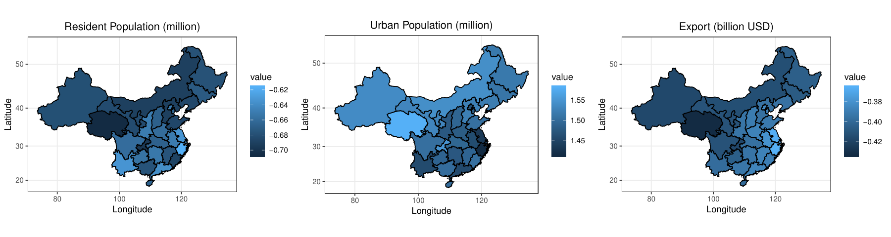
Under the GWR model with a Gaussian weighting scheme, the posterior modes of the indicators are , respectively, which indicates that the covariates , and are selected, while covariates and can be excluded from the regression model. Specifically, in our model, the number of resident population, the number of urban population, and total export value can help explain the change of GDP in each province. The posterior estimation results of the parameters under the Bayesian GWR model with a Gaussian weighting scheme are presented in Figure 5. The geographical variation in the parameters is rather obvious. We can see that the number of resident population and the total export value have significant negative impact on the increase of GDP, while the number of urban population has significant positive impact. For the Gaussian weight function, the posterior estimate of the bandwidth is 9.40, which indicates that the most distant provinces are assigned a relative weight of 0.665 in the estimation for one particular province. The impact of resident population on GDP is larger in north China than in southeast China. Comparing this to the population density map in China made by the Center for Geographic Analysis at Harvard University (worldmap.havard.edu/maps/11756), it can be seen that the influence is bigger in less populous provinces, which is in accordance with our intuition. The increasing effect of urban population on GDP is smaller in southeast China than in northwest China. Considering the relatively higher urbanization in south and east China (Wang et al. 2012), this can be explained by the “decreasing marginal effect” in economics. Export appears to be more important to provinces in west China than in eastern areas, which can also be explained by the fact that east China is relatively more developed, and have a more diversified source of GDP.
For comparison, classical frequentist GWR in (2) is also fitted on the dataset. We report the parameter estimates, together with plots, in the supplemental material. Particularly, the two covariates dropped by our Bayesian variable selection approach have the smallest absolute parameter values among all five covariates, which indicates that our proposed approach is indeed capable of picking out the most influential factors. The parameter estimates are also plotted on maps as in Figure 5. There are slight differences in the values of parameter estimates, which is partly due to the fact that we only have 150 observations (30 provinces, 5 years). It is, however, worth noticing that the trend of variation is consistent between the frequentist and Bayesian approaches.
Discussion
We developed a likelihood-based Bayesian approach to estimate regression coefficients in conjunction with spike and slab variable selection for geographically sparse data. The selection of bandwidth is discussed for a wide choice of weighting schemes using popular Bayesian model selection criteria such as the DIC and the LPML under the GWR context. The proposed methods are implemented in nimble. In our simulation studies, when there is no spatially varying covariate effect, the bandwidth is selected to give all observations close to uniform weight in estimating the coefficients for each individual location, whereas when there is indeed spatially varying covariate effect, the bandwidth is selected to achieve a balance between introducing bias for each location by taking into consideration nearby observations, and having too unstable estimates by placing the majority of emphasis on local observations and weighing down all others too heavily. The parameters estimated for each location have decent coverage rate that are close to the nominal 95% level.
Compared to the great circle distance, with a natural threshold of 1 to define “close enough”, the graph distance yields weighting schems that produce models with robust parameter estimation and variable selection performance. Based on comparisons with classical frequentist GWR from the simulation studies, it is interesting for us to notice that the bandwidth selection results of the Bayesian approach are different from that of the frequentist approach. A partial reason for this pattern is that the bandwidth selection of frequentist approach is based on minimizing the summation of the sum of square errors (SSE) for each locations. Our Bayesian approach, however, tries to maximize the whole data likelihood. Therefore, the frequentist approach tends to select smaller bandwidth than Bayesian approach.
A few issues beyond the scope of this paper are worth further investigation. In this work, we are only concerned with estimation of parameter for linear regression. Extension of similar ideas to generalized linear models, and semi-parametric models such as the Cox model, are worth developing. In the second alternative simulation scenario with regional variation patterns, both the frequentist and Bayesian GWR try to weigh neighbors as high as possible, leading to large bandwidths. Under the frequentist framework, clustering of covariate effects have been done using hierarchical clustering on the parameter estimation, which is ad hoc. Another approach is the penalized methods in Li and Sang 2019. In the Bayesian paradigm, however, hierarchical modeling provides an integrated framework that incorporates the latent cluster configuration layer. Development of such a framework is worth investigating. Also, we are assuming that a covariate is either in the true model for all locations, or not in the true model for all locations. There are cases where a covariate is important for some locations, but is minimally impacting for other locations. Identifying such locations is devoted to future research. Detecting a relationship between two areas that do not share a boundary (Gao and Bradley 2019) other than using graph distance is also an interesting future work.
References
- Bhattacharyya and Bickel (2014) Bhattacharyya, S. and P. J. Bickel (2014). Community detection in networks using graph distance. arXiv preprint arXiv:1401.3915.
- Boehm Vock et al. (2015) Boehm Vock, L. F., B. J. Reich, M. Fuentes, and F. Dominici (2015). Spatial variable selection methods for investigating acute health effects of fine particulate matter components. Biometrics 71(1), 167–177.
- Boscardin and Gelman (1993) Boscardin, W. J. and A. Gelman (1993). Bayesian computation for parametric models of heteroscedasticity in the linear model. In T. B. Fomby and R. C. Hill (Eds.), Advances in Econometrics, Volume 11, pp. 87–109. Emerald Group Publishing Ltd.
- Brunsdon et al. (1996) Brunsdon, C., A. S. Fotheringham, and M. E. Charlton (1996). Geographically weighted regression: a method for exploring spatial nonstationarity. Geographical Analysis 28(4), 281–298.
- Brunsdon et al. (1998) Brunsdon, C., S. Fotheringham, and M. Charlton (1998). Geographically weighted regression. Journal of the Royal Statistical Society: Series D (The Statistician) 47(3), 431–443.
- Brunsdon et al. (2000) Brunsdon, C., S. Fotheringham, and M. Charlton (2000). Geographically weighted regression as a statistical model. Technical report, Department of Geography, University of Newcastle-upon-Tyne.
- Cox and Cox (2000) Cox, T. F. and M. A. Cox (2000). Multidimensional Scaling. Chapman and Hall/CRC.
- da Silva and Fotheringham (2016) da Silva, A. R. and A. S. Fotheringham (2016). The multiple testing issue in geographically weighted regression. Geographical Analysis 48(3), 233–247.
- de Valpine et al. (2017) de Valpine, P., D. Turek, C. J. Paciorek, C. Anderson-Bergman, D. T. Lang, and R. Bodik (2017). Programming with models: writing statistical algorithms for general model structures with NIMBLE. Journal of Computational and Graphical Statistics 26(2), 403–413.
- Fotheringham et al. (2002) Fotheringham, A., C. Brunsdon, and M. Charlton (2002). Geographically Weighted Regression: The Analysis of Spatially Varying Relationships. Wiley. Chichester, West Sussex (UK).
- Fotheringham et al. (1998) Fotheringham, A. S., M. E. Charlton, and C. Brunsdon (1998). Geographically weighted regression: a natural evolution of the expansion method for spatial data analysis. Environment and Planning A 30(11), 1905–1927.
- Gao and Bradley (2019) Gao, H. and J. R. Bradley (2019). Bayesian analysis of areal data with unknown adjacencies using the stochastic edge mixed effects model. Spatial Statistics 31, 100357.
- Gelman et al. (2013) Gelman, A., H. S. Stern, J. B. Carlin, D. B. Dunson, A. Vehtari, and D. B. Rubin (2013). Bayesian Data Analysis. Chapman and Hall/CRC.
- George and McCulloch (1993) George, E. I. and R. E. McCulloch (1993). Variable selection via Gibbs sampling. Journal of the American Statistical Association 88(423), 881–889.
- Hu and Huffer (2020) Hu, G. and F. Huffer (2020). Modified Kaplan-–Meier estimator and Nelson-–Aalen estimator with geographical weighting for survival data. Geographical Analysis 52(1), 28–48.
- Ibrahim et al. (2013) Ibrahim, J. G., M.-H. Chen, and D. Sinha (2013). Bayesian Survival Analysis. Springer Science & Business Media.
- Ishwaran et al. (2005) Ishwaran, H., J. S. Rao, et al. (2005). Spike and slab variable selection: frequentist and Bayesian strategies. The Annals of Statistics 33(2), 730–773.
- LeSage (2004) LeSage, J. P. (2004). A Family of Geographically Weighted Regression Models, pp. 241–264. Berlin, Heidelberg: Springer Berlin Heidelberg.
- Li and Sang (2019) Li, F. and H. Sang (2019). Spatial homogeneity pursuit of regression coefficients for large datasets. Journal of the American Statistical Association 114(527), 1050–1062.
- Ma et al. (2018) Ma, Z., M.-H. Chen, and G. Hu (2018). Bayesian hierarchical spatial regression models for spatial data in the presence of missing covariates with applications. Technical Report 18-22, University of Connecticut, Department of Statistics.
- Mei et al. (2006) Mei, C.-L., N. Wang, and W.-X. Zhang (2006). Testing the importance of the explanatory variables in a mixed geographically weighted regression model. Environment and Planning A 38(3), 587–598.
- Müller et al. (1987) Müller, W., K. Szymanski, J. Knop, and N. Trinajstić (1987). An algorithm for construction of the molecular distance matrix. Journal of Computational Chemistry 8(2), 170–173.
- Páez et al. (2002a) Páez, A., T. Uchida, and K. Miyamoto (2002a). A general framework for estimation and inference of geographically weighted regression models: 1. location-specific kernel bandwidths and a test for locational heterogeneity. Environment and Planning A 34(4), 733–754.
- Páez et al. (2002b) Páez, A., T. Uchida, and K. Miyamoto (2002b). A general framework for estimation and inference of geographically weighted regression models: 2. spatial association and model specification tests. Environment and Planning A 34(5), 883–904.
- Shao (1997) Shao, J. (1997). An asymptotic theory for linear model selection. Statistica Sinica 7(2), 221–264.
- Spiegelhalter et al. (2002) Spiegelhalter, D. J., N. G. Best, B. P. Carlin, and A. Van Der Linde (2002). Bayesian measures of model complexity and fit. Journal of the Royal Statistical Society: Series B (Statistical Methodology) 64(4), 583–639.
- Tobler (1970) Tobler, W. R. (1970). A computer movie simulating urban growth in the Detroit region. Economic Geography 46(sup1), 234–240.
- Wang et al. (2012) Wang, L., C. Li, Q. Ying, X. Cheng, X. Wang, X. Li, L. Hu, L. Liang, L. Yu, H. Huang, and P. Gong (2012, Aug). China’s urban expansion from 1990 to 2010 determined with satellite remote sensing. Chinese Science Bulletin 57(22), 2802–2812.
- Wang et al. (2008) Wang, N., C.-L. Mei, and X.-D. Yan (2008). Local linear estimation of spatially varying coefficient models: an improvement on the geographically weighted regression technique. Environment and Planning A 40(4), 986–1005.
- Wooldridge (2015) Wooldridge, J. M. (2015). Introductory Econometrics: A Modern Approach. Nelson Education.
- Xue et al. (2019) Xue, Y., E. D. Schifano, and G. Hu (2019). Geographically weighted Cox regression and its application to prostate cancer survival data in Louisiana. Geographical Analysis. Forthcoming.