Estimating Extreme Value Index by Subsampling for Massive Datasets with Heavy-Tailed Distributions

1. INTRODUCTION

Extreme value theory (EVT) is an elegant probability theory for describing the asymptotic behavior of sample extremes (e.g., maximum or minimum). It has profound applications in many research fields. Those fields include but are not limit to risk management in geoscience (Katz et al., 2002; An and Pandey, 2005), finance (Gillia and Këllezib, 2006) and public health (Thomas et al., 2016). We refer to Coles, 2001 and Beirlant et al., 2004 for an excellent summary.

One problem of major interests in extreme value theory is to infer rare extreme events. An example is the estimation of the high-level quantiles for the unknown population distribution. In this paper, we focus on high-level quantile estimation for univariate heavy-tailed distributions. Mathematically, we refer to the distribution function with polynomially decaying tail as heavy-tailed (Hall, 1982; Wang and Tsai, 2009; Sun et al., 2020). Specifically, we assume that for a random variable $X$ following a heavy-tailed distribution $F$, there exist two positive constants $\beta$ and $\gamma$ such that

as $x\rightarrow\infty$. By the EVT, we know that the sample maximum in this case should follow a Fréchet type extreme value distribution asymptotically. A list of commonly used heavy-tailed distributions satisfy (1.1), including Student’s t, Pareto and Fréchet distributions; see Section 3.1 for their specific distribution functions. The shape of the tail distribution is mainly determined by an extreme value index $\gamma>0$ (de Haan and Ferreira, 2006). Once the parameter $\gamma$ (together with $\beta$ and some other necessary parameters) is consistently estimated, we can obtain the consistent estimations for the high-level quantiles and tail probabilities additionally.

Various estimators for the extreme value index $\gamma$ have been proposed. Some widely-used examples include the Hill estimator (Hill, 1975) for $\gamma>0$, the maximum likelihood estimator (Smith, 1985; Smith, 1987) for $\gamma>-1/2$, the probability weighted moment method (Hosking et al., 1985) for $\gamma<1/2$ and the moment method (Dekkers et al., 1989) for general $\gamma\in\mathbb{R}$. All those pioneer estimation methods have been found useful in the traditional setup, where the dataset is of moderate size. Nevertheless, the story changes in the context of massive datasets. Here massive datasets refer to the type of datasets, which are too large to be read into a typical computer’s memory as a whole. For instance, the default size of RAM pre-installed in a standard MacBook Pro is up to 16 GB. Hence the datasets of sizes larger than (or even close to) 16 GB can hardly be loaded into the computer’s memory as a whole. Thus, they can be regarded as massive for this particular computer. Massive datasets are becoming increasingly available due to the speedy advances of information technology. For datasets of massive sizes, they are often high-dimensional. In this case, the extreme value index needs to be estimated separately for each individual feature. A direct solution is to load the whole dataset in a part-by-part manner. Then estimators on each part are computed separately and finally aggregated to form a final estimator (Seila, 1982; Tafazzoli and Wilson, 2010; Alexopoulos et al., 2019). However, this solution may lead to high time cost since we have to process all the data points. See the time cost for analyzing a real massive dataset as reported in Figure 6 for example.

To circumvent this issue, one option is to implement a distributed parallel computing system to analyze the whole dataset in a divide-and-conquer manner (Lin and Xi, 2011; Chen and Xie, 2014; Jordan et al., 2019). However, the complexity and luxury of a distributed system makes this approach not suitable for all scenarios. Another convenient option is to draw subsamples from the whole dataset to adapt to limited computational resources and time budgets (Fithian and Hastie, 2014; Ma et al., 2015; Wang et al., 2018; Wang and Ma, 2021). Although subsampling may suffer from statistical efficiency reduction since it only involves a small part of data information, it is practically very attractive due to the significant benefits in terms of time savings. The savings can then be transferred to statistical gains in other aspects. For example, we can experiment with a broader range of candidate models in limited time budgets and update model promptly to accommodate ever-changing conditions.

In this paper, we develop a subsample-based methodology to estimate the extreme value index. The general idea is to draw random subsamples with replacement from the entire dataset such that the subsamples can be loaded into the memory as a whole. To obtain a more accurate estimation, subsampling can be performed for multiple times. With the help of subsamples, the classical peaks over threshold (POT) method (Davison and Smith, 1990) is carefully studied. Accordingly, an approximate maximum likelihood estimator for the extreme value index can be computed for each subsample. Next, estimators obtained from different subsamples are averaged together so that a more powerful estimator can be constructed. We refer to the final estimator as the averaged maximum likelihood (AML) estimator. The consistency and the asymptotic normality of our new estimator are also established. Based on the AML estimator, we are able to estimate high-level quantiles for the underlying data distribution consistently.

It is noteworthy that although multiple subsamples are involved in our approach, the number of subsamples can be relatively small if the execution efficiency is the major concern (which is often the case in real applications). Therefore, the overall amount of data points included in all subsamples is still much smaller compared to the whole dataset. This leads to a significant reduction in computation and data loading overhead. In fact, as we will elaborate in Sections 2 and 3, the number of subsamples is allowed to be varied within a wide range. Its value can be determined according to several factors including the whole dataset size, the memory capacity, expected statistical accuracy and time budgets. Consequently, the tuning parameter selection in our method is more practical and flexible for massive data analysis.

The rest of this paper is organized as follows. Section 2 introduces an averaged maximum likelihood method and investigates its asymptotic properties. Numerical studies are given in Section 3. A real airline dataset analysis is included in Section 4. Finally, the paper is concluded with a brief discussion in Section 5. All the proofs, together with additional lemmas, are deferred to the Appendix.

2. THE METHODOLOGY

2.1. Averaged Maximum Likelihood Estimation

Let $X_{i}$’s $\in\mathbb{R}\ (i=1,2,\cdots,N)$ be independent and identically distributed copies of a random variable $X\in\mathbb{R}$ with cumulative distribution function $F$. In this work, we focus on heavy-tailed distributions only. We follow the tradition (Hall, 1982; Wang and Tsai, 2009; Sun et al., 2020) and assume that the decaying rate of the distribution’s tail probability is polynomial. Specifically, we assume that $F$ satisfies (1.1). This suggests that high-level quantiles estimates can be obtained as long as the parameter $\gamma$ (or plus $\beta$) can be consistently estimated.

To estimate the extreme value index $\gamma$, a classical method is to model the conditional excess probability over a high threshold. This technique is called the peaks over threshold (POT) method (Davison and Smith, 1990). Specifically, for a random variable $X$ satisfying (1.1) and a given high threshold $u$, it can be shown that

for $t>1$. In other words, the exceedances over the high threshold $u$ can be approximated by a Generalized Pareto distribution with shape parameter $\gamma$ (Pickands III, 1975; Coles, 2001).

Inspired by the classical POT method, we develop here a subsample-based counterpart. To this end, denote the index set of the full dataset as $\mathbb{S}=\left\{1,\cdots,N\right\}$. We randomly draw $K$ subsamples of size $n$ with replacement from the full dataset. For the $k$-th subsample ($1\leq k\leq K$), the correspnding index set is denoted as $\mathcal{S}_{k}=\{m^{(k)}_{1},m^{(k)}_{2},\cdots,m^{(k)}_{n}\}\subset\mathbb{S}$. Conditioning on $\mathbb{S}$, $\{m^{(k)}_{i}:1\leq i\leq n,1\leq k\leq K\}$ are independent and identically distributed with $P(m^{(k)}_{i}=j)=1/N$ for any $j\in\mathbb{S}$. Let $f(x|u)$ be the probability density function of $X$ given $X>u$. By (2.1), $f(x|u)=(\gamma u)^{-1}(x/u)^{-1/\gamma-1}+o(1)$ for $u\rightarrow\infty$ and $x>u$. Then we can derive the following approximate log-likelihood function for the $k$-the subsample as

By maximizing $\mathcal{T}_{k}(\gamma)$ with respect to $\gamma$, we get an approximate maximum likelihood estimator as $\hat{\gamma}_{k}=\arg\max\limits_{\gamma}\mathcal{T}_{k}(\gamma)=(n_{k}^{u})^{-1}\sum_{i\in\mathcal{S}_{k}}\log(X_{i}/u)I(X_{i}>u)$. Here, $n_{k}^{u}=\sum_{i\in\mathcal{S}_{k}}I(X_{i}>u)$ is the number of observations over a pre-defined threshold $u$ for the $k$-th ($1\leq k\leq K$) subsample. We then combine these subsample-based estimators together. This leads to the averaged final estimator

We refer to $\hat{\gamma}_{\text{\sc aml}}$ as the averaged maximum likelihood (AML) estimator. As we can see, the AML estimator is closely related to the classical Hill estimator (Hill, 1975) in this setting. A more general combination scheme is to use the weighted average of $\hat{\gamma}_{k}$s. For example, the weight for subsample $\mathcal{S}_{k}$ can be selected to be proportional to $n_{k}^{u}$ or its transformation. This leads to much improved finite sample performance if unequal subsample sizes are allowed. See Section 3.2 for numerical evidences.

2.2. Theoretical Properties

To investigate the asymptotic behavior of $\hat{\gamma}_{k}$ and the averaged estimator $\hat{\gamma}_{\text{\sc aml}}$, the following conditions are needed.

• (C1)

  (Tail Probability) Define $\alpha_{u}=P(X>u)$. Assume that as $u\rightarrow\infty$, there exists a set of fixed constants $\beta>0,\gamma>0,\delta>0$ and $C\in\mathbb{R}$ such that $\alpha_{u}=\beta u^{-1/\gamma}\left\{1+Cu^{-\delta}+\\ o(u^{-\delta})\right\}$.

• (C2)

  (Subsample Ratio) As $N\rightarrow\infty$, assume that $n\rightarrow\infty$ and $n=o(N)$.

• (C3)

  (Divergence Rate) As $N\rightarrow\infty$, we assume that the threshold $u$ satisfies $u\rightarrow\infty$, $un^{-\gamma}\rightarrow 0$ and $un^{-\gamma/(2\delta\gamma+1)}\rightarrow\infty$.

• (C4)

  (Number of Subsamples) As $N\rightarrow\infty$, we assume that $K=o(\min\{n^{-1}u^{1/\gamma+2\delta},nu^{-1/\gamma}\})$.

Condition (C1) quantifies the decaying speed of the tail probability. A similar condition has been popularly assumed in extreme value literature (Hall, 1982; Smith, 1987; Resnick, 2007; Wang and Tsai, 2009). It is equivalent to replace $\beta$ and $C$ in Condition (C1) by two smooth functions $\beta(u)$ and $C(u)$ respectively, as long as $\beta(u)\rightarrow\beta$ and $C(u)\rightarrow C$ as $u\rightarrow\infty$. Condition (C2) is widely used in subsampling literature (Kleiner et al., 2014; Wang et al., 2018; Wang and Ma, 2020). It enforces that the subsample size $n$ should diverge to infinity at an appropriate speed. Specifically, $n$ should not be too small. Otherwise, the asymptotic theory cannot be developed. On the other hand, $n$ should not be too large. Otherwise the subsample is too large to be loaded into memory. Condition (C3) imposes a restriction on the divergence speed of the threshold level $u$. On the one side, it should not be too small. Otherwise the tail probability cannot be well approximated by the polynomial function as given in Condition (C1). On the other side, it cannot be too large either. Otherwise the exceedance size of each subsample $n_{k}^{u}$ is too small to support a consistent estimator. Condition (C4) implies that the number of subsamples $K$ can be either a fixed integer or diverge to infinity but not too fast. Obviously, larger $K$ leads to smaller variability of $\hat{\gamma}_{\text{\sc aml}}$. Since the local estimators $\hat{\gamma}_{k}$s are identically distributed, $\hat{\gamma}_{\text{\sc aml}}$ shares the same amount of bias as $\hat{\gamma}_{k}$. Accordingly, the bias of $\hat{\gamma}_{\text{\sc aml}}$ cannot be reduced by increasing $K$. As a consequence, if $K$ is too large, the bias suffered by $\hat{\gamma}_{\text{\sc aml}}$ becomes nonnegligible, as compared with its standard deviation. Consequently, the number of subsamples $K$ cannot be too large either. Otherwise the benefit introduced by larger $K$ in terms of variability reduction can be completely offset by its bias.

According to Theorem 1, we know that both the local estimator $\hat{\gamma}_{k}$ and the averaged estimator $\hat{\gamma}_{\text{\sc aml}}$ are consistent and asymptotically normal. The rate of convergence is $\sqrt{n_{k}^{u}}$ for $\hat{\gamma}_{k}$ and $\sqrt{n_{*}^{u}}$ for $\hat{\gamma}_{\text{\sc aml}}$, respectively. To make inference about $\gamma$, consider a confidence level $1-\alpha$. An asymptotically valid confidence interval for $\gamma$ can be constructed as $\hat{\gamma}_{\text{\sc aml}}\pm\Phi^{-1}(1-\alpha/2)\hat{\gamma}_{\text{\sc aml}}/\sqrt{n_{*}^{u}}$, where $\Phi$ is the cumulative distribution function of the standard normal distribution. In the meanwhile, assume a high threshold $u>0$, (2.1) indicates that $P(X>x)\approx\alpha_{u}\left(x/u\right)^{-1/\gamma}$ for any $x>u$. Therefore, for a quantile level $1-\tau$ with sufficiently small positive $\tau$, we have $P(X>q^{(a)}_{1-\tau})\approx\tau$ with $q^{(a)}_{1-\tau}=u\left(\alpha_{u}/\tau\right)^{\gamma}$. Denote the exact $(1-\tau)$-th quantile of distribution $F$ as $q_{1-\tau}$. That is $P(X>q_{1-\tau})=\tau$. We should expect $q^{(a)}_{1-\tau}\approx q_{1-\tau}$. A natural estimator for $q^{(a)}_{1-\tau}$ is given by $\hat{q}^{(a)}_{1-\tau}=u\left(\hat{\alpha}_{u}/\tau\right)^{\hat{\gamma}_{\text{\sc aml}}}$ with $\hat{\alpha}_{u}=(nK)^{-1}n_{*}^{u}$, provided $\tau<\alpha_{u}$. This leads to a useful method to approximate the high-level quantile for $X$, if $\gamma$ can be consistently estimated. Let $\hat{\tau}=P(X>\hat{q}^{(a)}_{1-\tau})$, The following theorem describes the asymptotic behavior of $\hat{q}^{(a)}_{1-\tau}$ and $\hat{\tau}$.

Theorem 2 indicates that we can estimate a very high-level quantile $q_{1-\tau}$ consistently. The resulting tail probability $\hat{\tau}$ is also ratio-consistent for the intended tail probability. It is remarkable that this can be done even if $\tau$ is too small to have sufficient number of extreme observations (i.e. $X_{i}$s such that $X_{i}>q_{1-\tau}$). Take an example for illustration. Consider a low level $\tau=10^{-5}$. To estimate the corresponding quantile $q_{1-\tau}$, very large sample size (e.g. $N\gg 10^{5}$) is needed if a traditional nonparametric method is used. However, under the help of $\hat{\gamma}_{\text{\sc aml}}$, we can estimate $q_{1-\tau}$ consistently with $K=10$ and $n=10^{3}$. Accordingly, the tail probability $\tau$ can also be estimated consistently.

3. NUMERICAL STUDIES

3.1. Simulation Models

To demonstrate the finite sample performance of the proposed estimators, we conduct a number of simulation studies in this section. To this end, we need to generate $X_{i}$s from a distribution whose tail probability satisfies Condition (C1). Specifically, we consider the following examples.

Example 1. (Student’s t-distribution) The first example considered here is the student’s t-distribution. It has been popularly used in extreme value modeling literature (Blattberg and Gonedes, 1974; Stoyanov et al., 2011). The distribution is heavy-tailed on both sides (right and left). Specifically, let $X$ follow a Student’s t-distribution with $v$ degrees of freedom, then the right tail probability becomes (Beirlant et al., 2004)

Consequently, the corresponding extreme value index is given by $\gamma=1/v$. The degree of freedom parameter $v$ controls the tail behavior of the Student’s t-distribution. In this simulation study, we consider Student’s t-distributions with $v=1$ and $v=2$, denoted as $t(1)$ and $t(2)$.

Example 2. (Pareto distribution) Pareto distribution is another widely adopted heavy-tailed distribution. It is found to be particularly useful in income distribution research (Wold and Whittle, 1957; Nirei and Aoki, 2016). The right tail probability of $\text{Pareto}(x_{m},\alpha)$ where $\alpha>0$ is given by $P(X>u)=(u/x_{m})^{-\alpha}$ with $u\geq x_{m}$ . Accordingly, the extreme value index is given by $\gamma=1/\alpha$. Specially, the parameter $C$ in Condition (C1) is equal to 0. The tail heaviness is controlled by the parameter $\alpha$. In this simulation study, we consider cases $\text{Pareto}(2,1)$ and $\text{Pareto}(2,2)$.

Example 3. (Fréchet distribution) We study here the Fréchet distribution. The tail probability of $\text{Fr\'{e}chet}(\alpha)$ where $\alpha>0$ is given by $P(X>u)=1-\exp(-u^{-\alpha})=u^{-\alpha}\left\{1-0.5u^{-\alpha}+o(u^{-\alpha})\right\}$. As a consequence, the extreme value index is given by $\gamma=1/\alpha$. Thus, the tail behavior of a Fréchet distribution is determined by $\alpha$. In this simulation study, we consider Fréchet(1) and Fréchet(2) cases.

Example 4. (Multimodal distribution) We consider in this example a multimodal distribution. Inspired by Cao and Zhang, 2020, we adopt the following method to generate $X_{i}$s from a heavy-tailed multimodal distribution. Specifically, $\{X_{i}\}_{i=1}^{N}$ is independently generated by $X_{i}=\max\{Y_{i},Z_{i}\}$, where $Y_{i}$ and $Z_{i}$ are independently generated from Fréchet(1) and Gumbel(8,8), respectively. Here, $\text{Gumbel}(\alpha,\beta)$ refers to the Gumbel distribution with tail probability $P(Z>u)=1-\exp\{-\exp{(Z-\alpha)/\beta}\}$. It is obvious that the tail probability of the Gumbel distribution diverges to zero exponentially. As a consequence, it can be shown that $X_{i}$s satisfies Condition (C1). The corresponding extreme value index is determined by the Fréchet part and thus equals to 1. The density function of $X_{i}$ is plotted in Figure 1, which is multimodal.

Example 5. (Non-independent data) We consider here a non-independent data example. Assume that $\{X_{i}\}_{i=1}^{N}$ are partitioned into $m$ clusters. The $k$-th cluster contains $N_{k}$ random variables, which is denoted by $\{X_{k1},\cdots,X_{kN_{k}}\},1\leq k\leq m$. For cluster $k$, $X_{kj}$ is generated by $X_{kj}=\alpha_{k}+\varepsilon_{kj},1\leq j\leq N_{k}$. This is a standard random effects model, where the random effect parameter $\alpha_{k}$ is generated from Fréchet(1) and the random noise $\varepsilon_{kj}$ is generated from $N(0,1)$. Consequently, $X_{kj}$s within the same cluster are correlated. It can be verified that the tail behavior of $X_{kj}$ is mainly decided by $\alpha_{k}$. Thus, the corresponding extreme value index is 1.

The above examples specify the generating distribution for $X$. Once the generating distribution and the whole sample size $N$ are given, we can simulate the full dataset. Here, we consider different $N$ values for different examples. For Examples 1–3, we set $N=10^{5},5\times 10^{5},10^{6},5\times 10^{6}$. While for Examples 4–5, we set $N=10^{7},4\times 10^{7},7\times 10^{7},10^{8}$. In view of Condition (C2) requiring that $n=o(N)$, we set $n=\lfloor N^{0.5}\rfloor$. Here, $\lfloor x\rfloor$ stands for the largest integer no larger than $x$. Condition (C3) requires that $u=n^{\gamma/(1+h\gamma)}$ with $h\in(0,2\delta)$. It implies that $P(X>u)=O(n^{-1/(1+h\gamma)})$. Therefore, the threshold value is set to be the $(1-n^{-1/(1+h\gamma)})$-th quantile of the given generating distribution. We fix $h=0.8\delta$ for Examples 1–3 and $h=0.6\delta$ for Examples 4–5. Moreover, Condition (C4) indicates that the divergence speed of $K$ is at most $o(n^{\delta/(\gamma^{-1}+\delta)})$. Hence, we let $K=\lfloor n^{C_{K}\delta/(\gamma^{-1}+\delta)}\rfloor$ with coefficients $C_{K}$=0.3, 0.5, 0.7 (for Examples 1–3) or $C_{K}$=0.3, 0.4, 0.5 (for Examples 4–5). The parameter $\delta$ of Examples 1–5 is set to be 2, 5, $\alpha$, 1 and 1 respectively. Thereafter, the averaged estimator $\hat{\gamma}_{\text{\sc aml}}$ can be computed.

3.2. Simulation Results

To obtain a reliable evaluation, we randomly replicate each simulation experiment for a total of $R=1,000$ times. Let $\hat{\gamma}_{\text{\sc aml}}^{(r)}$ be the averaged estimator obtained in the $r$-th ($1\leq r\leq R$) replication. We then define the root mean squared error (RMSE) as

Additionally, an asymptotic $1-\alpha$ confidence interval for $\gamma$ can be constructed as $\text{CI}^{(r)}=\Big(\hat{\gamma}_{\text{\sc aml}}^{(r)}-\Phi^{-1}(1-\alpha/2)\hat{\gamma}_{\text{\sc aml}}^{(r)}/\sqrt{n_{*(r)}^{u}},\hat{\gamma}_{\text{\sc aml}}^{(r)}+\Phi^{-1}(1-\alpha/2)\hat{\gamma}_{\text{\sc aml}}^{(r)}/\sqrt{n_{*(r)}^{u}}\Big)$. Then the empirical coverage probability is given by $\text{ECP}=R^{-1}\sum_{r=1}^{R}I(\gamma\in\text{CI}^{(r)})$. Here we fix $\alpha=0.05$. We can further obtain a $(1-\tau)$-th quantile estimator for $X$ in the $r$-th replication as $\hat{q}^{(a,r)}_{1-\tau}$. We can compute the tail probability $\hat{\tau}^{(r)}=P\big(X>\hat{q}^{(a,r)}_{1-\tau}\big)$ according to its theoretical formula. This leads to relative accuracy (RA) for tail probability as

In this simulation study, we set $\tau=10^{-3}$.

The simulation results are summarized in Tables 1–4 (in Appendix B). First, we find that the RMSE of $\hat{\gamma}_{\text{\sc aml}}$ decreases towards 0 as the whole exceedances size $n_{*}^{u}$ increases for all the examples. In particular, the standard deviation decreases towards 0 as $n_{*}^{u}$ goes to infinity. However, with a fixed whole sample size $N$, the bias of $\hat{\gamma}_{\text{\sc aml}}$ has little changes as the number of subsamples $K$ increases. This is expected because the bias is mainly controlled by $n_{*}^{u}$ and has nothing to do with $K$. Second, the empirical coverage probabilities (ECP) are all quite close to the nominal level 95%. This confirms the asymptotical normality of $\hat{\gamma}_{\text{\sc aml}}$. Additionally, the relative accuracy of the tail probability estimator (the last column) approaches 0 as $n_{*}^{u}$ increases towards infinity. This corroborates the theoretical findings given in Theorem 2. Additionally, although we require that $K$ goes to infinity in Condition (C4), the simulation results shows that in practice, a relative small $K$ (corresponds to $C_{K}=0.3$) is large enough for a practically acceptable statistical performance. Hence, if the statistical consistency of the estimator and execution efficiency is the major concern (which is indeed often the case in practice), then a relatively small $K$ can be used.

We next evaluate the performance of two different combination schemes in terms of $\hat{\gamma}_{k}$s. Apart from the simple average based estimator as we introduced in Section 2.1, we also consider to use a weighted average of $\hat{\gamma}_{k}$s to form the final estimator. Specifically, the weight for the $k$-th subsample is proportional to its exceedance size $n_{k}^{u}$. We select $t(1)$ as the generating function and follow a similar model setup as stated in Section 3.1. Specifically, we set $N=10^{6},5\times 10^{6},10^{7}$ and $n=\lfloor N^{0.5}\rfloor$. The number of subsamples $K$ is set to be $K=10,14,20$ respectively . The threshold value $u$ satisfies $P(X>u)=O(n^{-1/(1+2h)})$ with $h=0.8$. We consider two different scenarios regarding the subsample size $n_{k}$. The first scenario is a balanced case with $n_{k}=n$ for each $k$. The second scenario is an imbalanced case with $n_{k}=1.5n$ for $1\leq k\leq K/2$ and $n_{k}=0.5n$ for $1+K/2\leq k\leq K$. We replicate the simulation for 1,000 times and report the results in Table 5. It can be seen that estimators produced by the simple average and weighted average schemes perform similarly, if equal subsample sizes are used. In contrast, the weighted average estimator performs much better than the simple average one, if very different subsample sizes are allowed.

3.3. The Competing Estimators

For comparison purpose, we also evaluate here a number of competing estimators. They are, respectively, the probability weighted moment estimator (Hosking and Wallis, 1987) and the moment estimator (Dekkers et al., 1989). These two methods are constructed according to the method of moments. In contrast, our estimator is developed based on the approximate likelihood (Estimating Extreme Value Index by Subsampling for Massive Datasets with Heavy-Tailed Distributions
) and is more closely related to the Hill estimator (Hill, 1975). Thus, the classical Hill estimator is not included for comparison. Similar to the AML estimator, the moment estimator and the probability weighted moment estimator of $\gamma$ can be computed on each subsample. This leads to a total of $K$ estimators. They are then averaged to form the final ones. The resulting estimators are referred to as an averaged probability weighted moment (APWM) estimator and an averaged moment (AMO) estimator respectively. Specifically, for the $k$-th subsample, let $X^{(k)}_{1:n}\leq X^{(k)}_{2:n}\leq\cdots\leq X^{(k)}_{n:n}$ denote the order statistics. Then the APWM estimator is given by

where $P_{n}^{(k)}=(n_{k}^{u})^{-1}\sum_{i=1}^{n_{k}^{u}}X^{(k)}_{n-i+1:n}-u$, $Q_{n}^{(k)}=(n_{k}^{u})^{-1}\sum_{i=1}^{n_{k}^{u}}\{(i-1)/(n_{k}^{u}-1)\}(X^{(k)}_{n-i+1:n}-u)$. The AMO estimator is given by

where $M_{n,l}^{(k)}=(n_{k}^{u})^{-1}\sum_{i=1}^{n_{k}^{u}}(\log X^{(k)}_{n-i+1:n}-\log u)^{l}$, $l=1,2$.

Note that the classical probability weighted moment estimator is consistent only for $\gamma<1$ and is asymptotically normal only for $\gamma<1/2$. For a fair comparison, we only consider here generating distributions with $\gamma<1/2$. Specifically, those distributions are t(3), t(5), Pareto(2,3), Pareto(2,5), Fréchet(3) and Fréchet(5), respectively. The whole sample size $N$ varies form $10^{6}$ to $10^{7}$. The subsample size $n$ is fixed at $n=\lfloor N^{0.5}\rfloor$. The number of subsamples is given by $K=10$. The threshold value $u$ is set to be the $(1-n^{-0.6})$-th quantile of $X$. We compare the RMSE values of $\hat{\gamma}$ for three different estimation methods (AML, AMO and APWM). The simulation results are shown in Figure 2. From Figure 2, we can observe that the AML estimator always performs best in all cases.

However, it is remarkable that the optimal threshold value for different estimators could be different. Thus, comparing the performance of different estimators under one pre-specified threshold value might be unconvincing. To address the issue, we fix $N=5\times 10^{6}$ and $n=\lfloor N^{0.5}\rfloor=2,236$. We compare the best finite sample performances of the three estimators. That is their minimal RMSE values across a wide range of threshold values. In this study, a total of 50 threshold values are considered. Their corresponding tail probabilities are given by $0.5+i/100$ for $i=0,1\cdots,49$. We present the detailed results in Figure 3. As one can see, the minimal RMSE values of the AML estimators remain the smallest.

3.4. Threshold Selection

We now consider the problem of the threshold selection for the AML estimation. As we pointed out earlier in Section 2.2, it is critical to specify an appropriate $u$. On the one hand, $u$ should be sufficiently large to ensure that the error in approximating tail probability by Condition (C1) is small enough. On the other hand, larger $u$ corresponds to small exceedance size (i.e., $n_{*}^{u}$), which leads to poor statistical performances of AML estimators. In this section, we follow Wang and Tsai, 2009 and provide here a simple but effective framework to select the threshold $u$ adaptively. Concretely, note that given a proper $u$, the distribution of $\gamma^{-1}\log(X/u)$ conditional on $X>u$ is approximately standard exponential. This implies that the distribution of $\exp\{-\gamma^{-1}\log(X/u)\}$ conditional on $X>u$ is approximately a uniform distribution on $[0,1]$. As a result, an optimal threshold value $u$ should be the one corresponding to the minimal distance between the uniform distribution on $[0,1]$ and the empirical distribution of $\{\hat{Z}_{i}:X_{i}>u,i\in\cup_{k=1}^{K}\mathcal{S}_{k}\}$, where $\hat{Z}_{i}=\exp\{-(\hat{\gamma}_{\text{\sc aml}})^{-1}\log(X_{i}/u)\}$.

There are many methods to quantify the distance between the empirical distribution of the sample and the reference distribution. One popular method is to apply the Cramér-von Mises statistic (Choulakian and Stephens, 2001). Based on a total of $K$ subsamples, it can be calculated as follows:

where $n_{*}^{u}=\sum_{k}n_{k}^{u}=\sum_{k}\sum_{i\in\mathcal{S}_{k}}I(X_{i}>u)$ denotes the size of total exceedances as defined in Theorem 1. $\hat{Z}_{i:n_{*}^{u}}$ represents the $i$-th order statistic of $\{\hat{Z}_{i}\}$ with $\hat{Z}_{1:n_{*}^{u}}\leq\hat{Z}_{2:n_{*}^{u}}\leq\cdots\leq\hat{Z}_{n_{*}^{u}:n_{*}^{u}}$. Note that if $\hat{Z}_{i:n_{*}^{u}}$ is indeed uniformly distributed on $[0,1]$, then the value $W^{2}(u)$ should be small. Hence, we suggest that the optimal threshold value $u$ can be selected as $u_{1}^{*}=\mbox{argmin}_{u}W_{1}^{2}(u)$. Note that the computation scheme of (3.3) requires going through $K$ subsamples twice. To reduce time overhead costs, a simpler scheme is to calculate $W^{2}$ based on the first subsample $\mathcal{S}_{1}$, where the corresponding selected threshold value is defined as $u_{2}^{*}$. For elaboration convenience, we refer to the procedures of selecting $u_{1}^{*}$ and $u_{2}^{*}$ as Scheme 1 and Scheme 2 respectively.

To evaluate the performance of these two schemes in $u$ selection, we consider to generate simulated dataset from distributions t(1) and t(2). The whole sample size $N$ varies from $10^{4}$ to $10^{5}$. The subsample size $n$ is fixed at $n=\lfloor N^{0.5}\rfloor$. The number of subsamples $K$ is fixed at $K=\lfloor n^{0.4}\rfloor$ and $K=\lfloor n^{0.6}\rfloor$ respectively. We consider a total of 100 candidate values for $u$, with the corresponding empirical tail probabilities (based on the first subsample) are evenly distributed on the interval [0.005,0.5]. Then we perform the two different schemes to select the optimal value of $u$. These lead to two different values of AML estimator. Figure 4 presents the RMSEs of AML estimators over 100 replications. As expected, Scheme 1 outperforms Scheme 2 by a noticeable margin. It is better to use Scheme 1 for threshold selection. However, since Scheme 2 only needs to go through all subsamples once, Scheme 2 might be practically more convenient if the time budget is extremely limited.

4. THE AIRLINE DATA ANALYSIS

To demonstrate the practical usefulness of the proposed method, we present here a real dataset analysis. The dataset is referred to as the airline data. It can be freely downloaded from the website http://stat-computing.org/dataexpo/2009/. Each record contains detailed information for one particular commercial flight within the USA, from 1987 and 2008. Specifically, a total of 29 variables are included in each record. Among these variables, 13 of them are continuous variables. However, most of these continuous variables suffer from severe missing problems. Therefore, we will only focus on four continuous variables with missing rates less than 10% for illustration purpose. They are, respectively, the ActualElapsedTime (actual elapsed time), CRSElapsedTime (scheduled elapsed time), ArrDelay (arrival delay) and DepDelay (departure delay) variables. More details about these variables can be found in the downloading website.

Our aim in this study is to obtain the 99.99% quantiles of the underlying distributions that corresponds to these four continuous variables respectively. Note that the original dataset contains about 120 million (116,525,241) records. It takes up about 12 GB on a hard drive. As a consequence, it is too large to be read into a usual personal computer’s memory as a whole. We have to rely on subsampling technique for data analysis. To achieve the best subsampling efficiency, we need to preprocess the data on the hard drive appropriately. In particular, the physical address of each data line on the hard drive should be handled carefully. Otherwise, the pointer of the data reader cannot be located to the starting position for each data line efficiently. The preprocessing and subsampling procedures have been developed into an off-the-shelf python module. It is publicly available online at https://github.com/holybadger/clubear. With the aid of the python module, we first randomly draw a subsample with size $n=10,000$ for a quick review. Based on the subsample, we are able to calculate the kurtosis for each variable. The detailed results are reported in Table 6 (in Appendix B). From Table 6, we can see that all the variables have kurtosis larger than 3. While the kurtosis of the ArrDelay and DepDelay variables are larger than 9. This indicates that all the five variables under study have heavier tails than a normal distribution. Moreover, two of them are even more severely heavy-tailed compared with $t(5)$. The outlier detection for these variables becomes imperative and challenging.

To address the issue, we use the proposed subsampling-based method to estimate the upper and lower bound of for each variable. The number of subsamples and each subsample size are mainly determined by the memory capacity, expected statistical accuracy and time budgets. In this analysis, we fix $n=10,000$ and $K=100$, which is $O(N^{0.5})$ and $O(n^{0.5})$ respectively. Before the formal data analysis, the original data are appropriately centered so that its tail distribution can be better approximated by the tail probability which specified in Condition (C1). To determine the threshold value $u$, we consider a total of 100 candidate values, with the corresponding empirical tail probabilities (based on the first subsample) evenly distributed on the interval $[0.005,0.5]$. As discussed in Section 3.4, we select the threshold value that minimizes the Cramér-von Mises statistic value for each variable. Specifically, the optimal threshold values for ActualElapsedTime, CRSElapsedTime, ArrDelay and DepDelay are the 98.5%, 98.0%, 99.5%, 99.5% empirical quantiles, respectively. To assess the goodness-of-fit, we employ the quantile-quantile (Q-Q) plot. If the threshold value is selected properly, then the transformed random variables $\hat{Z}_{i}$s will be expected to be uniformly distributed on $U[0,1]$. Hence, the corresponding Q-Q plot should approximately follow a 45-degree straight line. Figure 5 displays the Q-Q plots corresponding to the selected optimal threshold value for each variable. They all approximately follow a 45-degree straight line. Hence, we conclude that the selected threshold values are satisfactory.

Given the threshold value, we can calculate $\hat{\gamma}_{k}$ for each subsample and finally obtain the AML estimator $\hat{\gamma}_{\text{\sc aml}}$. Then we are able to compute the value of the quantile estimator $\hat{q}^{(a)}_{1-\tau}$ according to its formula. The quantile level $\tau$ is fixed to be $10^{-4}$. In other words, for each variable, $99.99\%$ of the normal records are expected to be no more than $\hat{q}^{(a)}_{1-\tau}$. Hence, the value of $\hat{q}^{(a)}_{1-\tau}$ can be served as an upper bound for each variable. Observations that fall outside the bound will be considered as suspected outliers and be treated separately. From Table 6, we observe that, for all variables under study except DepDelay, less than 0.01% of observations are detected as suspected outliers. However, for DepDelay, the suspected outlier probability becomes 0.011%, which is larger than the nominal level 0.01%. This suggests that for DepDelay, some of those suspected outliers deserve our attention. Their extreme behaviors can hardly be explained by the inherent tail-heaviness of the data distribution. Therefore, practically it needs further and more careful analysis to investigate whether these points are genuine outliers or highly influential observations.

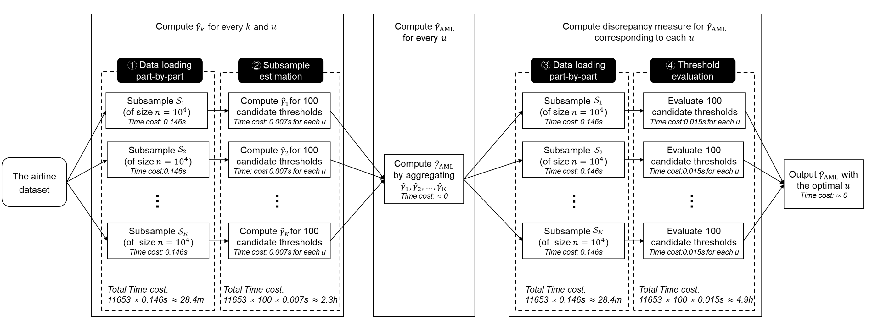
Lastly, we compare the total time cost between the subsampling based method and the whole data based method. Note that the airline dataset is too large to be loaded into memory as a whole. Consequently, if the whole data based estimator is to be computed, it has to be partitioned into many non-overlapping small pieces. Subsequently these small pieces can be processed in a part-by-part manner. For convenience, we refer to each small piece as a subsample and fix the subsample size to be $n=10,000$. This leads to a total of 11,653 non-overlapping subsamples. Our numerical experiment suggests that it takes about 2.5 seconds on average to finish all the necessary computation jobs for each subsample. This includes the time costs for data loading, parameter estimation for a total of 100 candidate threshold values, and threshold evaluation according to the discrepancy measure, as developed in Section 3.4. Consequently, if the whole dataset is to be processed, the total time cost is about $11,653\times 2.5$ seconds $\approx 8$ hours. In contrast, for our proposed subsampling method, the total time cost can be significantly reduced to be $K\times 2.5$ seconds with $K=100$ (less than 5 minutes). A workflow chart in this regard is illustrated in Figure 6. The whole dataset based global estimators (denoted as $\hat{\gamma}_{\text{global}}$) and the subsample based estimators (i.e., $\hat{\gamma}_{\text{AML}}$) for the four interested variables are reported in Table 6. We find that the absolute differences between $\hat{\gamma}_{\text{global}}$ and $\hat{\gamma}_{\text{AML}}$ are less than $0.12\%$ for all variables. It seems to us that such a difference is tiny and practically very acceptable for most real applications.

5. CONCLUDING REMARKS

In this paper, we develop a subsampling-based method to estimate the extreme value index for heavy-tailed data. The method is developed particularly for massive datasets with memory constraints. By repeatedly subsampling from the whole data, we can estimate the extreme value index consistently. With the help of the extreme value index estimator, the corresponding estimations for high-level quantiles and tail probabilities can also be obtained. The analysis from both simulated and real datasets demonstrates the effectiveness and efficiency of the method. Moreover, this method does not require luxury computing devices, such as parallel computing servers. It is more flexible and available for most practitioners with limited computing resources.

To conclude this paper, we would like to discuss a number of interesting problems for further research. First, it would be worthy to extend our method to multivariate settings. Since the large-scale data in reality are often high-dimensional, the tail dependence between different variables might be nonnegligible. The way to take this information into consideration deserves further investigation. Second, recall that in this paper, $X_{i}$s are assumed to be independent and identically distributed random variables with extreme value index $\gamma$. Let $\xi$ be an arbitrary but fixed constant. Theoretically speaking, both variables $X_{i}$ and $X_{i}+\xi$ should have the same extreme value index. Accordingly, the interested extreme value index can be estimated by either the original sample $\{X_{i}\}$ or the shifted one $\{X_{i}+\xi\}$. Both samples should lead to consistent estimators for $\gamma$. However, our numerical experience suggests that their finite sample performances could be very different. An appropriately shifted sample can yield an estimator substantially more efficient than that of the original one. As a consequence, how to select the optimal shifting parameter should be another interesting topic for future study. Third, apart from uniform subsampling, a series of novel non-uniform subsampling methods have also been developed in recent years (Ma et al., 2015; Wang et al., 2018; Han et al., 2020; Ai et al., 2021; Wang and Ma, 2021). For non-uniform sampling, it generally aims to approximate the whole dataset based estimators by selecting informative observations with higher probabilities. Thus, it leads to more efficient estimators with a fixed subsample size. Developing a similar method for estimating the extreme value index will be a useful and interesting research topic, which is worth further exploration.

APPENDIX A. LEMMAS

In this section, we present here several useful lemmas for proofs of theorems in Appendix B. To prove the first conclusion in Theorem 1, the following lemma is needed. Similar lemma was also developed in Wang and Tsai, 2009. The difference is that the lemma given in Wang and Tsai (2009) was developed for original data while ours is developed for subsampled data. The details are given below.

To prove the second conclusion in Theorem 1, we need the following three lemmas. We first develop an Bernstein-type inequality for subsampled data in Lemma 2. This lemma can be viewed as the extension of the classical Bernstein inequality (Bennett, 1962) but for subsampled data.

REFERENCES

- Ai et al., (2021) Ai, M., Yu, J., Zhang, H., and Wang, H. (2021). Optimal subsampling algorithms for big data regressions. Statistica Sinica, 31:749–772.
- Alexopoulos et al., (2019) Alexopoulos, C., Goldsman, D., Mokashi, A. C., Tien, K.-W., and Wilson, J. R. (2019). Sequest: A sequential procedure for estimating quantiles in steady-state simulations. Operations Research, 67(4):1162–1183.
- An and Pandey, (2005) An, Y. and Pandey, M. (2005). A comparison of methods of extreme wind speed estimation. Journal of Wind Engineering and Industrial Aerodynamics, 93(7):535–545.
- Beirlant et al., (2004) Beirlant, J., Goegebeur, Y., Segers, J., and Teugels, J. L. (2004). Statistics of Extremes: Theory and Applications. John Wiley & Sons.
- Bennett, (1962) Bennett, G. (1962). Probability inequalities for the sum of independent random variables. Journal of the American Statistical Association, 57(297):33–45.
- Blattberg and Gonedes, (1974) Blattberg, R. C. and Gonedes, N. J. (1974). A comparison of the stable and student distributions as statistical models for stock prices. The Journal of Business, 47(2):244–280.
- Cao and Zhang, (2020) Cao, W. and Zhang, Z. (2020). New extreme value theory for maxima of maxima. Statistical Theory and Related Fields, 0(0):1–21.
- Chen and Xie, (2014) Chen, X. and Xie, M. (2014). A split-and-conquer approach for analysis of extraordinarily large data. Statistica Sinica, 24(4):1655–1684.
- Choulakian and Stephens, (2001) Choulakian, V. and Stephens, M. A. (2001). Goodness-of-fit tests for the generalized pareto distribution. Technometrics, 43(4):478–484.
- Coles, (2001) Coles, S. (2001). An Introduction to Statistical Modeling of Extreme Values. Springer Science & Business Media.
- Davison and Smith, (1990) Davison, A. C. and Smith, R. L. (1990). Models for exceedances over high thresholds. Journal of the Royal Statistical Society: Series B, 52(3):393–425.
- de Haan and Ferreira, (2006) de Haan, L. and Ferreira, A. (2006). Extreme Value Theory: An Introduction. Springer Science & Business Media.
- Dekkers et al., (1989) Dekkers, A., Einmahl, J., and de Haan, L. (1989). A moment estimator for the index of an extreme-value distribution. The Annals of Statistics, 17(4):1833–1855.
- Fithian and Hastie, (2014) Fithian, W. and Hastie, T. (2014). Local case-control sampling: Efficient subsampling in imbalanced data sets. The Annals of Statistics, 42(5):1693–1724.
- Gillia and Këllezib, (2006) Gillia, M. and Këllezib, E. (2006). An application of extreme value theory for measuring financial risk. Computational Economics, 27(2-3):207–228.
- Hall, (1982) Hall, P. (1982). On some simple estimates of an exponent of regular variation. Journal of the Royal Statistical Society: Series B, 44(1):37–42.
- Han et al., (2020) Han, L., Tan, K. M., Yang, T., and Zhang, T. (2020). Local uncertainty sampling for large-scale multiclass logistic regression. The Annals of Statistics, 48(3):1770–1788.
- Hill, (1975) Hill, B. M. (1975). A simple general approach to inference about the tail of a distribution. The Annals of Statistics, 3(5):1163–1174.
- Hosking and Wallis, (1987) Hosking, J. R. and Wallis, J. R. (1987). Parameter and quantile estimation for the generalized pareto distribution. Technometrics, 29(3):339–349.
- Hosking et al., (1985) Hosking, J. R. M., Wallis, J. R., and Wood, E. F. (1985). Estimation of the generalized extreme-value distribution by the method of probability-weighted moments. Technometrics, 27(3):251–261.
- Jordan et al., (2019) Jordan, M. I., Lee, J. D., and Yang, Y. (2019). Communication-efficient distributed statistical inference. Journal of the American Statistical Association, 114(526):668–681.
- Katz et al., (2002) Katz, R. W., Parlange, M. B., and Naveau, P. (2002). Statistics of extremes in hydrology. Advances in Water Resources, 25(8-12):1287–1304.
- Kleiner et al., (2014) Kleiner, A., Talwalkar, A., Sarkar, P., and Jordan, M. I. (2014). A scalable bootstrap for massive data. Journal of the Royal Statistical Society: Series B, 76(4):795–816.
- Lin and Xi, (2011) Lin, N. and Xi, R. (2011). Aggregated estimating equation estimation. Statistics and Its Interface, 4(1):73–83.
- Ma et al., (2015) Ma, P., Mahoney, M. W., and Yu, B. (2015). A statistical perspective on algorithmic leveraging. The Journal of Machine Learning Research, 16(1):861–911.
- Nirei and Aoki, (2016) Nirei, M. and Aoki, S. (2016). Pareto distribution of income in neoclassical growth models. Review of Economic Dynamics, 20:25–42.
- Pickands III, (1975) Pickands III, J. (1975). Statistical inference using extreme order statistics. The Annals of Statistics, 3(1):119–131.
- Resnick, (2007) Resnick, S. I. (2007). Heavy-Tail Phenomena Probabilistic and Statistical Modeling. Springer Science & Business Media.
- Seila, (1982) Seila, A. F. (1982). A batching approach to quantile estimation in regenerative simulations. Management Science, 28(5):573–581.
- Smith, (1985) Smith, R. L. (1985). Maximum likelihood estimation in a class of nonregular cases. Biometrika, 72(1):67–90.
- Smith, (1987) Smith, R. L. (1987). Estimating tails of probability distributions. The Annals of Statistics, 15(3):1174–1207.
- Stoyanov et al., (2011) Stoyanov, S. V., Rachev, S. T., Racheva-Yotova, B., and Fabozzi, F. J. (2011). Fat-tailed models for risk estimation. The Journal of Portfolio Management, 37(2):107–117.
- Sun et al., (2020) Sun, Q., Zhou, W.-X., and Fan, J. (2020). Adaptive huber regression. Journal of the American Statistical Association, 115(529):254–265.
- Tafazzoli and Wilson, (2010) Tafazzoli, A. and Wilson, J. R. (2010). Skart: A skewness-and autoregression-adjusted batch-means procedure for simulation analysis. IIE Transactions, 43(2):110–128.
- Thomas et al., (2016) Thomas, M., Lemaitre, M., Wilson, M. L., Viboud, C., Yordanov, Y., Wackernagel, H., and Carrat, F. (2016). Applications of extreme value theory in public health. PLoS One, 11(7):1–7.
- Wang and Ma, (2020) Wang, H. and Ma, Y. (2020). Optimal subsampling for quantile regression in big data. arXiv preprint arXiv:2001.10168.
- Wang and Ma, (2021) Wang, H. and Ma, Y. (2021). Optimal subsampling for quantile regression in big data. Biometrika, 108(1):99–112.
- Wang and Tsai, (2009) Wang, H. and Tsai, C.-L. (2009). Tail index regression. Journal of the American Statistical Association, 104(487):1233–1240.
- Wang et al., (2018) Wang, H., Zhu, R., and Ma, P. (2018). Optimal subsampling for large sample logistic regression. Journal of the American Statistical Association, 113(522):829–844.
- Wold and Whittle, (1957) Wold, H. O. and Whittle, P. (1957). A model explaining the pareto distribution of wealth. Econometrica, 25(4):591–595.