Time Evolution Of Cyclotron Line of Her X-1; A Detailed Statistical Analysis Including New ASTROSAT Data 2020Time Evolution Of Cyclotron Line of Her X-1; A Detailed Statistical Analysis Including New ASTROSAT Data–6
Abstract
The cyclotron line feature in the X-ray spectrum of the accretion powered pulsar Her X-1 has been observed and monitored for over three decades. The line energy exhibited a slow secular decline over the period 1995-2014, with a possible (not confirmed) indication of a reversal thereafter. Recent works have shown that the temporal evolution of the line energy may be modelled as a flattening after an earlier decrease until MJD 55400 (. In this work, we present the results of ASTROSAT observations in the context of earlier data and offer a common interpretation through a detailed study of temporal and flux dependence. We find that the variation of the line energy does not support an upward trend but is consistent with the reported flattening after an earlier decrease until MJD .
Keywords:
pulsars: general - X-rays: binaries - X-rays1 Introduction
Cyclotron Resonance Scattering Features (CRSF), also referred to as Cyclotron Lines, constitute an important tool for measuring the magnetic field strength of accreting neutron stars in X-ray binary systems. A long-term study of the cyclotron line can reveal the evolution of the magnetic field in the x-ray emitting region. In the highly magnetized plasma accumulated on the neutron star polar caps, the cyclotron lines are produced by resonant scattering of photons off electrons moving perpendicular to the magnetic field, and appear as absorption features against the X-ray continuum. The line energy () is related to the magnetic field as keV, where is the field strength in units of Gauss, and is the gravitational red shift.
Her X-1 is a 1.24 s period accretion-powered X-ray pulsar in a 1.7 day circular orbit with a normal stellar companion, HZ Her. The edge-on view of the accretion flow in this system reveals a rich variety of temporal and spectral features, which have been the subject of concerted study over many years. In addition to the basic spin and orbital periodicity, this binary system has been known to display a 35 day long cycle which consists of a "Main-On" (high X-ray flux) and a "Short-On" states, separated by two "Off" states (Jones & Forman 1976; Staubert et al. 2013). The sharp increase of the flux ("turn on") indicates the beginning of a cycle. This generally takes place either around binary phase 0.2 or 0.7. The cyclotron line in Her X-1 or in an X-ray binary was first detected in a 1976 balloon observation (Trümper et al. 1977, Truemper et al. 1978). At present nearly 36 sources are known to exhibit CRSF in their X-ray spectra (Staubert et al. 2019). The source Her X-1 is known to exhibit a positive correlation between and the X-ray luminosity (Staubert et al. 2007). A long-term decay of in Her X-1 was first discovered by Staubert 2014. Before 1991 the mean cyclotron line energy was around 35 keV (derived using HEAO-A4, Mir-HEXE, and Ginga observations (Soong et al. 1990)). Subsequently a very high value of nearly 44 keV (mean of the values observed in 1993 and 1996) was noticed from CGRO/BATSE data (Freeman et al. 1996). There was no observation that captured the intervening rise. Later, observations with BeppoSax and RXTE in 1997 found the line energy to be around 40-41 keV (Gruber et al. 2001). A regular monitoring was initiated at this stage, and the accumulated data since 1996 appeared to show that has both luminosity and time dependence (Staubert et al. 2014), with a slow secular decay of line energy with time. Further observations with INTEGRAL, Suzaku and NuSTAR fit well with a model assuming a continued decay of until 2015, with a decay rate of keV/yr (Staubert et al. 2016). However in 2016 NuSTAR and INTEGRAL observations of Her X-1 began to indicate a possible upward trend in line energy (Staubert et al. 2017) (which is not confirmed so far), possibly similar to the jump observed between 1991 and 1993. A recent work with SWIFT/BAT data claims that may in fact have been constant since 2012, with an attendant change in its dependence on luminosity (Ji et al. 2019; Xiao et al. 2019).
In this work we investigate both the luminosity and the temporal dependence of of Her X-1, using all previous data and new observations from the Indian AstroSat mission. In section 2 we introduce AstroSat and its instruments, as well as the standard data reduction tools. In section 3 we give an account of the method we have followed to analyze the data. In section 4 we compare different models of evolution. In section 5 we present our results and discuss possible physical reasons behind the observed behaviour of cyclotron line energy. Errors, wherever quoted, correspond to 68% confidence levels, unless otherwise mentioned.
| Obs | Center | Duration | BAT count | ASM flux | |
| Date | MJD | (ks) | (cm-2s-1) | (counts/s) | (keV) |
| 21 Jan 2018 | 58141 | 59.6 | |||
| 30 Jun 2017 | 57934 | 35.4 | |||
2 Observations and Data Reduction
In this work we use two datasets obtained using AstroSat’s (Singh et al. 2014) Large Area X-ray Proportional Counters (LAXPC) (Agrawal et al. 2017) and the Soft X-ray Telescope (SXT) (Singh et al. 2017). AstroSat is India’s first multi-wavelength satellite, carrying detectors in the visible, near and far ultraviolet (NUV/FUV) as well as soft, medium and hard X-ray bands. AstroSat consists of five principal scientific instruments, (i) a Soft X-ray Telescope (SXT) (0.3-8.0 keV), (ii) three Large Area X-ray Proportional Counters (LAXPCs) (3.0-80.0 keV), (iii) a Cadmium-Zinc-Telluride Imager (CZTI) (25-200 keV), (iv) two Ultra-Violet Imaging Telescopes (UVITs), capable of observing the sky in the Visible, Near Ultraviolet and Far Ultraviolet regions of the electromagnetic spectrum and (v) three Scanning Sky Monitors (SSMs), to scan the sky for long term monitoring of bright X-ray sources and the detection of bright X-ray transients. AstroSat also carries on board a Charged Particle Monitor (CPM).
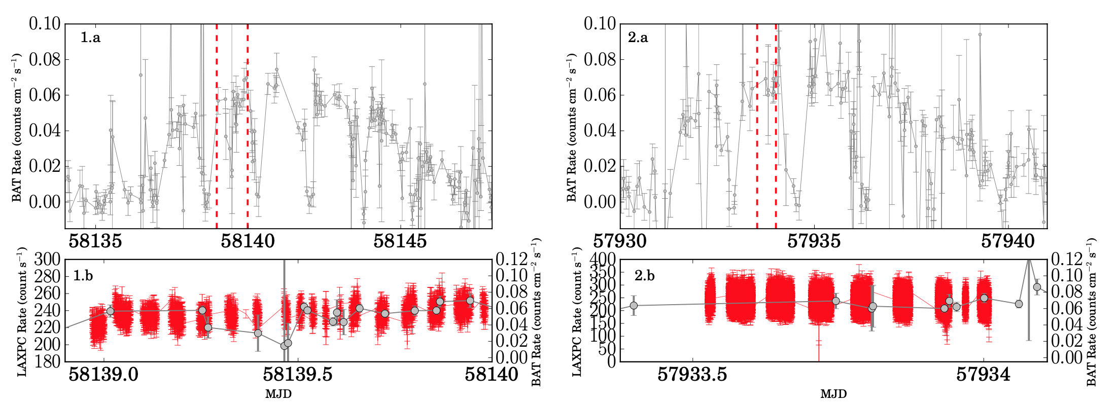
The first dataset in Table–1 was obtained from an observation proposed by us (ObsID 9000001854, PI: Suman Bala) and carried out over 20–22 Jan 2018, during the Main-On phase, avoiding eclipses. The second dataset (Obs ID: 9000001348, PI: Denis Leahy) carried out between 29-30 June 2017, was during a Main-On phase but also contains Main-on dips. Data points from the Main-on dips have been removed from our spectrum analysis. The datasets are retrieved from the AstroSat open public archive11 1 https://astrobrowse.issdc.gov.in/astro_archive/archive/Home.jsp. The AstroSat observation epochs are marked on the SWIFT/BAT lightcurve shown in the upper panel of Fig–1. BAT and LAXPC (15-50 keV) light curves within the AstroSat observation period are compared in the lower panel of Fig-1, showing similar variations.
2.1 Large Area X-ray Proportional Counters (LAXPC)
The LAXPC consists of a set of three non-imaging proportional counters (LXP10, LXP20, LXP30) nearly co-aligned with the satellite axis. The LAXPC operates in the energy range 3–80 keV with the energy resolution varying between 10% to 20%. A detailed description of the characteristics of the LAXPC instrument can be found in Antia et al. 2017.
For LAXPC, we use the level 1 data from the archive and the laxpcsoft package available at the AstroSat Science Support Cell (ASSC)22 2 http://astrosat-ssc.iucaa.in for analysis. First, we create a combined event file of all three LAXPC units using the standard procedure laxpc_make_event. After that we use laxpc_make_stdgti to generate a good time interval (gti) file, removing intervals of passage through the South Atlantic Anomaly (SAA) and Earth occultation. Using this gti file we create individual light-curves of each LAXPC unit (laxpc_make_lightcurve), and check for any anomalies in counts rates. We remove these anomalous intervals, all periods of binary eclipses and the time interval of absorption dips from the gti and create a filtered gti file for every LAXPC unit, as advised by the LAXPC instrument team. Finally we use the modified gti file to create spectra (using laxpc_make_spectra) for every individual LAXPC unit. The software also provides an appropriate grouping of the spectrum, oversampling the spectral resolution (15%) of the instrument by at most a factor of 3. The module laxpc_make_backspectra is used to generate the corresponding background spectrum, having gain close to our observation. The LAXPC pipeline creates the Response Matrix File (.rsp) corresponding to each observation and LAXPC unit. We further augment the response file with an additional Auxiliary Response File (ARF) created by us, as described in the Appendix–B.
At the time of our observations the LAXPC unit LXP30 had a rapidly changing gain due to a gas leak, and LXP20 had an uncertain spectral response caused by gas impurities and incomplete recording of Xenon K escape events. These two units were thus not suitable for accurate spectroscopic work. We therefore use data only from LXP10, in the energy range 5-60 keV since above 60 keV the background dominates and any error in background estimation can affect the spectrum significantly. Below 5 keV the background and the response of LAXPC are not yet fully understood and can leave unmodelled residuals in spectral fitting. For LAXPC10, the 5-60 keV net source count rates are counts/s and count/s respectively in the two datasets, and the corresponding background counts rates are counts/s and counts/s.
2.2 Soft X-ray imaging Telescope (SXT)
The SXT (Singh et al. 2017) is a focussing telescope with a focal length of 2 m and a thermo-electrically cooled CCD in the focal plane. Its operating energy range is 0.3–7.0 keV with an energy resolution eV at 6 keV. The field of view of SXT is of 40′ diameter with a Point Spread Function (PSF) of 2′ Full Width at Half Maximum (FWHM). The SXT observations used in this work have been carried out in the "Photon Counting" (PC) mode, where the data from the entire CCD of pixels are collected. Currently the lower energy threshold of SXT is set at 105 eV, above the electronic noise peak but the quantum efficiency of the detector is poorly determined below 0.7 keV. So, for our analysis, we have used the SXT Spectrum in the energy range 0.7–7.0 keV.
For SXT, we have used the level-2 data products from the archive. The level-2 data, namely the cleaned event files for individual orbits, are created by the SXT Payload Operation Centre (POC) using the SXTPIPELINE version-1.4a that takes care of time tagging of the events, calibration of the source events, the coordinate transformation from detector to sky coordinates, the pulse height amplitude (PHA) construction for each event, the conversion from the event PHA to pulse invariant (PI), bias subtraction and adjustment, flagging of the bad pixels and removal of hot and flickering pixels. We use a standard julia script, developed by the SXT instrument team, to create a single event file, by merging the event files of all orbits. A source region of 10 arcmin radius, which includes 90% of the source photons, has been selected from the image to generate the light curve and energy spectrum using the XSELECT task of HEASOFT33 3 https://heasarc.gsfc.nasa.gov/docs/software/heasoft/ version 6.25. We used the background file SkyBkg_comb_EL3p5_Cl_Rd16p0_v01.pha available at the ASSC. The updated response Matrix sxt_pc_mat_238new.rmf and Auxiliary Response File (ARF) sxt_pc_excl00_v04_mJ_final_scl.arf have been provided by G. C. Dewangan (private communication). The net SXT count rate for the dataset-1 and dataset-2 have been found to be and counts/s respectively, much less than the threshold ( 40 counts/s) above which the photon pile-up takes place. The SXT spectra have been binned considering at least 30 counts per energy bin.
3 Data Analysis
The hard X-ray continuum produced in the accretion column so far does not have any generally accepted physical model. In some special cases (e.g., for 4U 0115+63; Ferrigno et al. 2009), models based on the work by Becker & Wolff 2007 have been used to fit the continuum. Using the model of Becker & Wolff 2007, Wolff et al. 2016 has shown that the spectrum of Her X-1 obtained from a 2012 NuSTAR observation can be explained as continuum produced by a radiation dominated shock. Still, the model of Becker & Wolff 2007 has not been universally applied. It is therefore a common practice to use empirical models, like power law with an exponential roll over, to model the spectral continuum of X-ray pulsars. The continuum of Her X-1 is best described by a phenomenological power law with high-energy cutoff (highecut). Previous results of the long term evolution of the cyclotron line energy of Her X-1 have been reported using this continuum model. So, in this work we use the same model to fit the continuum for consistency.
The spectral analysis is done using XSPEC version: 12.10.0. From both the datasets, we have used the SXT data in the energy range of 0.7-7.0 keV and the LAXPC data in the range 5.0-60.0 keV. We have included a 2% systematic error in the SXT data and 1% in LAXPC data for the combined fitting (as recommended by the instrument teams). We have used the parameter constant to account for cross-instrument calibration uncertainties. The constant factor for LAXPC is frozen to 1.0 and for the SXT it is kept free. For SXT the gain adjustment with the slope fixed at 1 and an offset, has been kept free. A black body component (0.1 keV) and a Gaussian Iron line at keV have been used to model the combined spectrum. As the width of the iron line could not be constrained well, it has been frozen to the previously reported value of 0.22 keV from NuSTAR observations (Fuerst et al. 2013). A recent study of Her X-1 has shown the presence of an emission line at keV (Leahy & Chen 2019). Thus, we have included a Gaussian emission line around 0.94 keV in our combined fitting. The galactic absorption for Her X-1 is always found to be very low (Fuerst et al. 2013; Leahy & Chen 2019), whereas including a partial-covering absorber tbpcfabs (Wilms et al. 2000) improves the fit. The highecut model shows a sharp feature at the cutoff energy (e.g. Kretschmar et al. 1997, Kreykenbohm et al. 1999), and a Gaussian optical-depth profile (gabs) is often used to smooth it (e.g. Coburn et al. 2002; Fuerst et al. 2013). So, we have included a gabs with its energy tied to the cutoff energy, keeping the width and depth free. A cyclotron line feature is generally modeled with either a cyclabs or a gabs profile. Following earlier works, we have used a Gaussian optical-depth (gabs) to model the cyclotron line. The complete model used for the combined fit of LAXPC and SXT is,
| (1) | ||||
After fitting the LAXPC spectrum, we have observed some overall unmodelled residuals. This could be either due to a poor response function or inadequate background modelling. So, we fixed the continuum parameters at values derived after studying NuSTAR observations of Her X-1 (Staubert 2020, submitted to A&A). The continuum parameters corresponding to the observed flux during our observations are found to be, = 20.37 keV and 20.62 keV, = 10.1 keV and 10.15 keV and Photon Index = 0.99,0.99 for dataset-1 and dataset-2 respectively. At high energies the spectrum is found to deviate from the model, mostly due to improper modelling of LAXPC background spectra. To counter that we have used the original background spectra generated by LAXPC pipeline with an adjustable rescaling factor. The best fit is achieved when the original background spectra are rescaled by factors 1.05 and 1.04 for dataset-1 and dataset-2 respectively. We also find that at high energies the original background spectra deviate from the spectra obtained while Her X-1 was occulted by the Earth, and the same rescaling factors as above resolved those differences (Appendix–A). Even after this, we find some residuals in the overall LAXPC spectra, which are also observed in the LAXPC spectra of other strong sources. This systematic deviation may be attributed to the uncertainties in the response of LAXPC. So, we have created an Auxiliary Response (ARF), using the Crab spectrum, in an attempt to remove these artifacts. The details of the ARF have been given in Appendix–B. The ARF for dataset-1 has been created using a Crab spectrum observed on 16th Jan, 2018 (MJD 58134, 7 days before our observation) but for dataset-2 we did not find any near-by Crab observation so a corresponding ARF could not be created.
| Dataset-1 | Dataset-2 | ||
|---|---|---|---|
| Parameter | With | Without | Without |
| ARF | ARF | ARF | |
| (cm-2) | |||
| (keV) | |||
| (keV) | |||
| (keV) | |||
| (keV) | |||
| (keV) | |||
| (keV) | |||
| (keV) | |||
| (keV) | |||
| (keV) | |||
| /d.o.f | |||
Optical depth, .
*The parameter value is fixed.

For dataset-1, the cyclotron line energy is found to be keV, with a width of keV. The fit is found to improve significantly when the cyclotron feature is included, /d.o.f=542.9/529 compared to that without (/d.o.f=929.9/532). The best fit parameter values are given in Table–2. The table displays parameters both with and without the inclusion of the LAXPC ARF derived by us. For dataset-2 the line energy is found to be keV and the /d.o.f is found to be without the line and with the line. In both cases the line has been detected with more than confidence level. Fig–2 shows the unfolded spectra of Her X-1 and best fit delchi plots. We find that our line energies are consistent but the widths are lower than the expected, comparing with other measurements of NuSTAR (Staubert 2020, submitted to A&A). This indicates that further modification in the LAXPC response is required, which is beyond the scope of this work.
4 Variation of The Cyclotron line energy with luminosity and time
To examine the dependence of on luminosity and time we carried out a two parameter fit using the well known non-linear least squares fitting routine mpfit (Markwardt 2009). We have also used emcee, (a Goodman and Weare’s Affine Invariant Markov chain Monte Carlo (MCMC) Ensemble sampler (Foreman-Mackey et al. 2013)) for Bayesian parameter estimation with some suitable flat priors (Table–3). In this work, we have used all the data previously used in Staubert et al. 2014 and Staubert et al. 2017 and our recent AstroSat results. We use the cyclotron line energies derived without any flux or temporal correction.
To investigate the correlation between the line energy and flux, the Main-on flux has been computed by taking the average count rates of 3 days around the maximum of the cleaned main on phase obtained from Swift/BAT light-curve (as suggested in Appendix-A of Staubert et al. 2016). We find that the maximum Main-on flux corresponding to our AstroSat observations are and counts cm-2s-1 for dataset-1 and dataset-2 respectively. Using the scaling factor, [2-10 keV ASM-counts/s]=93.0[15-50 keV BAT-counts cm-2s-1] (Staubert et al. 2016), we find that the equivalent ASM-counts/s are and respectively.
We have described the variation of cyclotron line energy of Her X-1 by Eq–2.


| (2) |
Here, is the observed cyclotron line energy at a time (in MJD) and is the corresponding ASM Main-On flux. , , , , and are the fit parameters of our models. Here and are in the units of keV/d. Following earlier works, we set the value of the reference flux to 6.8 ASM-counts/s and the reference time to MJD 53500. We have chosen the parameter ranges in such a way as to reproduce and compare the results from all existing models (e.g. Staubert 2014; Ji et al. 2019 etc.), intending to find the best description for the variation of the cyclotron line energy of Her X-1. The best fit parameter values for all cases are tabulated in Table–3.
Case–I: In this case we assume, , , , , , . This implies that the cyclotron line energy does not depend explicitly on time, and the observed variation in the line energy is only due to the variation of the Main-On flux. With this model the best estimated /d.o.f is found to be 346.7/25. The best fit parameter values are given in Table–3.
Case–II: Here we assume, , , , , , . This implies that the cyclotron line energy has both flux and temporal dependence which is assumed to be the same throughout. This model gives a better fit than case–I, with a /d.o.f=77.9/24. This suggests the existence of an explicit temporal dependence.
Case–III: In this case we assume, , , , , , . So, there is both flux and temporal dependence until MJD 55400, after which the time dependence disappears and only the flux dependence remains. This model is equivalent to the model described in Ji et al. 2019. This model gives the /d.o.f to be 25.8/23.
Case–IV: In this case we assume, , , , , , . This is the same as case–III except that here is set to be MJD 57341 when the line energy is found to be minimum and a ’turn up’ is assumed (Staubert et al. 2017). The /d.o.f is found to be 26/23.
Case–V: In this case we assume, , , , , , . The difference between this and cases III and IV is that here the vale of is found by fitting. We find that this is the best model (/d.o.f=15.7/22) to describe the observed variation of cyclotron line energy in Her X-1. We find a fitted value of (=), close to the previously suggested value , by Ji et al. 2019. The distribution of model parameters of our Bayesian parameter estimator are shown in Fig–3.
Case–VI: In this case, , , , , , . The assumption is that the line energy depends both on time and flux and there is an explicit rise of with time after = 57341. This is equivalent to the model described in Staubert et al. 2017. With this model we find the /d.o.f to be 22/22, with =. This clearly shows that current observations do not support a recent turn-up after 2015.
Case–VII: In this case we assume, , , , , , . This is akin to case–VI but here the is found by fitting. In this case we get two degenerate solutions as shown in Fig–4. The degeneracy can be broken by considering two different ranges of ; i) (VII.a, Fig–5) and ii) (VII.b, Fig–6). We get two sets of parameter values VII.a and VII.b, (Table–2) with /d.o.f of 14.4/21 and 22/21 respectively. The parameter values of VII.b are found to be the same as in case–VI. The parameter values for case–VII.a are found to be close to those of case–V. The value of for VII.a is found to be keV/d, which is close to zero. The chance probability of case–VII.a being identical to case–V is found to be very high (0.18). Hence case–V is considered as the best model because it has fewer parameters.

So, We find the best fit when we assume that there is an initial decay of line energy with time, and after MJD , the line energy no longer has explicit temporal dependence (case–V). In Fig–7 we have shown all the data which are considered in our fitting and the behaviour of our model (Eq–2) for different cases. In this correlation analysis a few extreme outlier data points have been ignored (following Staubert et al. 2016) while carrying out the fitting. However the conclusions do not change even if all the observed data are included, albeit with a poorer reduced . The parameters estimated after including all the data points are given in Appendix–6.
All errors are reported with 1 (68%) confidence range.
| Case | [keV/- | (keV) | /d.o.f | F-values | Chance | ||||
| (keV) | ASM-counts/s] | [keV/d] | (keV) | MJD | [keV/d] | Probability | |||
| Range | [35, 45] | [0, 2] | [-20, 0] | [30, 45] | [50000, 59000] | [-20, 10] | |||
| I | - | - | - | - | |||||
| II | - | - | - | 77.9/24 | (I–II) 82.8 | ||||
| III | 55400 | - | 25.8/23 | (II–III) 46.4 | |||||
| IV | 57341 | - | 26/23 | (II–IV) 45.9 | |||||
| V | - | 15.7/22 | (II–V) 43.6 | ||||||
| VI | 57341 | - | - | ||||||
| VII.a | 14.4/21 | (V-VII.a) 1.9 | 0.18 | ||||||
| VII.b | 22/21 | - | - | ||||||
5 Discussion and conclusions
In our work we find that the currently available data do not support the idea of a recent trend of secular increase of the cyclotron line energy or the initiation of a new Turn-up phase of Her X-1. The sudden increase of cyclotron line energy with time has been seen in this source during 1990-1993 (Gruber et al. 2001). After that it was believed that a continuous and almost steady decay of cyclotron line energy with time occurred over a period of 20 years at a rate of keV yr-1 between 2004-2010 (Staubert et al. 2014). We have tested different models of the evolution of cyclotron line energy against the available data. We observe that the variation of cyclotron line energy in Her X-1 can be best described by a model that considers an initial decay of line energy after the sudden increase in 1990-1993, and then constancy after a time (Case–V). We determine to be in the range MJD , close to that reported in Ji et al. 2019. The relatively large uncertainty in is due to the lack of observations in the intervening period. With our best fit model (case–V), the coefficient of flux dependence is found to be keV/ASM-counts/s, close to the value reported by Staubert et al. 2007 at the discovery of the flux dependence (also used by Ji et al. 2019). However the decay rate keV/day is found in this case to be significantly different from the values reported earlier (Staubert 2014; Staubert et al. 2016; Ji et al. 2019). This is also seen in one other case (VII.a), among those explored by us.
As mentioned in section–1, and derived in the model fits above, Her X-1 exhibits a positive correlation between its luminosity and the cyclotron line energy. Several explanations have been offered in the literature for this behaviour (e.g. Staubert et al. 2007; Becker et al. 2012; Mushtukov et al. 2015). Among the causes cited, the most popular is the change in the height of the emission region above the neutron star surface with the accretion rate . A reduction in the height with increasing would lead to an increase in cyclotron line energy (Becker et al. 2012). Other possibilities include a change in the velocity distribution of infalling material and a consequent change in Doppler effect, as the accretion rate varies (Mushtukov et al. 2015). Mukherjee & Bhattacharya 2012 have shown that larger mass loading in the accretion column results in a greater distortion of the magnetic field lines, enhancing the field strength at the edge of the polar cap. This would lead to an increase in the cyclotron line energy, particularly if a fan beam emanating from the sides of the accretion column intercepts the observer.
The secular variation of line energy with time, however, still lacks a clear explanation (e.g. Staubert 2014). Possible reasons include a change in the intrinsic dipolar magnetic field strength of the neutron star and changes in the line forming region. The time scale for any appreciable change in the intrinsic dipole moment of the star is expected to be much larger (million years: Bhattacharya et al. 1992, Urpin et al. 1994) than the observed time scale of secular variation in line energy. An apparent reduction in the local magnetic field may therefore be attributed to a screening or burial of the magnetic field at the polar cap by continuous accretion (Cumming et al. 2001). Such a mechanism would then have to explain a decay rate of 0.2% per year in the local magnetic field strength, as implied by the observed change in the line energy. In this picture, a sudden increase of line energy could be due to a re-emergence of the buried field, but the relevant time scale for such emergence could be 100 years (Cumming et al. 2001; Sang & Chanmugam 1987) rather than a few years as seen in Her X-1. Staubert et al. 2017 explain the observed temporal variation of cyclotron line energy by considering the formation of an accretion mound at the polar cap region. In the accretion mound, there is a continuous inflow of material as well as an outflow due to the leakage of mater through magnetic field lines. If the inflow is greater than the outflow then the mound height increases which leads to the shifting of the line forming region away from the surface of neutron star, dragging the central field lines towards the edge. This reduces the magnetic field intensity of the line forming region, and hence a decay of the cyclotron line energy is expected in case of pencil beam emission (Mukherjee & Bhattacharya 2012). When the inflow and outflow of the material balance each other, a dynamic stability arises and the mound height as well as the cyclotron line energy becomes constant. If the accretion mound reaches a critical height, then instabilities in the accretion mound (Mukherjee et al. 2013a; Mukherjee et al. 2013b) may cause a sudden outflow of a substantial amount of matter. The reduction of the mound height and the consequent increase of the central field strength would then cause a sudden increase of the cyclotron line energy. This explanation would, however, contradict the observed positive correlation of line energy with luminosity. To explain the observed luminosity dependence with this model, the source Her X-1 needs to have a fan-beam emission as discussed in the previous paragraph.

We speculate that the positive correlation of the cyclotron line energy with luminosity reflects the change in the height of the emission region above the accretion mound (Becker et al. 2012), a larger accretion rate pushing the line forming region close to the mound surface. However, with time there is some accumulation of material at the polar cap, generally increasing the mound height. This is accompanied by a drop in the magnetic field intensity at the mound center as well as in the line forming region above the mound. Once the mound height achieves stability, the secular variation of the line energy would stop. We have extended the work of Mukherjee & Bhattacharya 2012 to Her X-1 and show the variation of the magnetic field strength at the top of the mound of different heights in Fig–8. We assume the shape of the mound to be parabolic with an intrinsic dipolar field strength G and solve the magnetostatic equilibrium for matter confined at the polar cap, as described in Mukherjee & Bhattacharya 2012. An increase in the height of the mound results in more magnetic flux being displaced from the centre towards the mound edge. If the radiation beam is axial and the cyclotron line carries the signature of the magnetic field near the centre of the polar cap, then with a larger mass loading the local field strength will reduce, causing the cyclotron line energy to drop. In our analysis, an 8% decrease in cyclotron line energy over time has been observed, which would be expected from the formation of a mound of height 60-70 m, reducing the central field to G. If a mound had been pre-existing, then the amount of increase in mound height required to cause a similar change may be obtained from the inset in Fig–8. We find that the maximum sustainable stable mound height (critical height) for Her X-1 can be 100 m, beyond which instabilities grow rapidly. Such a scenario may indeed be responsible for the observed behaviour of Her X-1. During 1990-1993, the mound might have reached its critical height, triggering a sudden outflow that reduced the mound height. This would cause an increase in the observed cyclotron line energy. After that the mound height starts to increase and the cyclotron line energy exhibits a secular decrease (1995 to 2009: case–V). Then as a dynamic stability between the inflow and the outflow of material is established, the mound height as well as the cyclotron line energy becomes constant. It is possible that in future if the inflow into the mound exceeds the outflow, then the mound can again grow to its critical height, triggering an instability in the mound. Regular monitoring of the cyclotron line energy of Her X-1 will be required to track such a behaviour and to estimate the timescale in which further changes in the line energy may occur.
Acknowledgements
The author, S. Bala wants to thank Dr Jayashree Roy, Prof. Ranjeev Misra and Prof. Gulab Chand Dewangan, Prof. Amit Shukla, Prof. Biswajit Paul and Dr Niladri Paul for their useful suggestions and discussions. The author would like to thank the anonymous referee for valuable suggestions to improve the work. The research work is funded by the University Grants Commission (UGC). The author wants to thank Inter University Center for Astronomy and Astrophysics (IUCAA) for the research facilities. This publication uses the data from the AstroSat mission of the Indian Space Research Organisation (ISRO), archived at the Indian Space Science Data Centre (ISSDC). This work has used the data from the LAXPC developed at TIFR, Mumbai, and the LAXPC POC at TIFR is thanked for verifying and releasing the data via the ISSDC data archive and providing the necessary software tools. This work has used the data from the Soft X-ray Telescope (SXT) developed at TIFR, Mumbai, and the SXT POC at TIFR is thanked for verifying and releasing the data via the ISSDC data archive and providing the necessary software tools. This research has made use of software and/or web tools obtained from the High Energy Astrophysics Science Archive Research Center (HEASARC), a service of the Astrophysics Science Division at NASA/GSFC and of the Smithsonian Astrophysical Observatory’s High Energy Astrophysics Division.
Data availability
The data underlying this article are publicly available in ISSDC, at https://astrobrowse.issdc.gov.in/astro_archive/archive/Home.jsp.
References
- Agrawal et al. (2017) Agrawal P. C., et al., 2017, Journal of Astrophysics and Astronomy, 38, 30
- Antia et al. (2017) Antia H. M., et al., 2017, ApJS, 231, 10
- Becker & Wolff (2007) Becker P. A., Wolff M. T., 2007, ApJ, 654, 435
- Becker et al. (2012) Becker P. A., et al., 2012, A&A, 544, A123
- Bhattacharya et al. (1992) Bhattacharya D., Wijers R. A. M. J., Hartman J. W., Verbunt F., 1992, A&A, 254, 198
- Coburn et al. (2002) Coburn W., Heindl W. A., Rothschild R. E., Gruber D. E., Kreykenbohm I., Wilms J., Kretschmar P., Staubert R., 2002, ApJ, 580, 394
- Cumming et al. (2001) Cumming A., Zweibel E., Bildsten L., 2001, ApJ, 557, 958
- Ferrigno et al. (2009) Ferrigno C., Becker P. A., Segreto A., Mineo T., Santangelo A., 2009, A&A, 498, 825
- Foreman-Mackey et al. (2013) Foreman-Mackey D., Hogg D. W., Lang D., Goodman J., 2013, Publications of the Astronomical Society of the Pacific, 125, 306–312
- Freeman et al. (1996) Freeman P. E., Lamb D. Q., Wilson R. B., Briggs M. S., Paciesas W. S., Preece R. D., Band D. L., Matteson J. L., 1996, in Kouveliotou C., Briggs M. F., Fishman G. J., eds, American Institute of Physics Conference Series Vol. 384, American Institute of Physics Conference Series. pp 172–176 (arXiv:astro-ph/9601167), doi:10.1063/1.51738
- Fuerst et al. (2013) Fuerst F., et al., 2013, preprint, (arXiv:1309.5361)
- Gruber et al. (2001) Gruber D. E., Heindl W. A., Rothschild R. E., Coburn W., Staubert R., Kreykenbohm I., Wilms J., 2001, ApJ, 562, 499
- Ji et al. (2019) Ji L., Staubert R., Ducci L., Santangelo A., Zhang S., Chang Z., 2019, MNRAS, 484, 3797
- Jones & Forman (1976) Jones C., Forman W., 1976, ApJ, 209, L131
- Kretschmar et al. (1997) Kretschmar P., et al., 1997, in Winkler C., Courvoisier T. J.-L., Durouchoux P., eds, ESA Special Publication Vol. 382, The Transparent Universe. p. 141
- Kreykenbohm et al. (1999) Kreykenbohm I., Kretschmar P., Wilms J., Staubert R., Kendziorra E., Gruber D. E., Heindl W. A., Rothschild R. E., 1999, A&A, 341, 141
- Leahy & Chen (2019) Leahy D. A., Chen Y., 2019, ApJ, 871, 152
- Madsen et al. (2017) Madsen K. K., Forster K., Grefenstette B. W., Harrison F. A., Stern D., 2017, ApJ, 841, 56
- Markwardt (2009) Markwardt C. B., 2009, in Bohlender D. A., Durand D., Dowler P., eds, Astronomical Society of the Pacific Conference Series Vol. 411, Astronomical Data Analysis Software and Systems XVIII. p. 251 (arXiv:0902.2850)
- Mukherjee & Bhattacharya (2012) Mukherjee D., Bhattacharya D., 2012, MNRAS, 420, 720
- Mukherjee et al. (2013a) Mukherjee D., Bhattacharya D., Mignone A., 2013a, MNRAS, 430, 1976
- Mukherjee et al. (2013b) Mukherjee D., Bhattacharya D., Mignone A., 2013b, MNRAS, 435, 718
- Mushtukov et al. (2015) Mushtukov A. A., Tsygankov S. S., Serber A. e. V., Suleimanov V. F., Poutanen J., 2015, MNRAS, 454, 2714
- Sang & Chanmugam (1987) Sang Y., Chanmugam G., 1987, ApJ, 323, L61
- Singh et al. (2014) Singh K. P., et al., 2014, in Space Telescopes and Instrumentation 2014: Ultraviolet to Gamma Ray. p. 91441S, doi:10.1117/12.2062667
- Singh et al. (2017) Singh K. P., et al., 2017, Journal of Astrophysics and Astronomy, 38, 29
- Soong et al. (1990) Soong Y., Gruber D. E., Peterson L. E., Rothschild R. E., 1990, ApJ, 348, 641
- Staubert (2014) Staubert R., 2014, preprint, (arXiv:1412.8067)
- Staubert (2020) Staubert R., 2020, A&A
- Staubert et al. (2007) Staubert R., et al., 2007, in The Obscured Universe. Proceedings of the VI INTEGRAL Workshop. p. 465
- Staubert et al. (2013) Staubert R., Klochkov D., Vasco D., Postnov K., Shakura N., Wilms J., Rothschild R. E., 2013, A&A, 550, A110
- Staubert et al. (2014) Staubert R., Klochkov D., Wilms J., Postnov K., Shakura N. I., Rothschild R. E., Fürst F., Harrison F. A., 2014, A&A, 572, A119
- Staubert et al. (2016) Staubert R., Klochkov D., Vybornov V., Wilms J., Harrison F. A., 2016, A&A, 590, A91
- Staubert et al. (2017) Staubert R., Klochkov D., Fürst F., Wilms J., Rothschild R. E., Harrison F., 2017, A&A, 606, L13
- Staubert et al. (2019) Staubert R., et al., 2019, A&A, 622, A61
- Truemper et al. (1978) Truemper J., Pietsch W., Reppin C., Voges W., Staubert R., Kendziorra E., 1978, ApJ, 219, L105
- Trümper et al. (1977) Trümper J., Pietsch W., Reppin C., Sacco B., 1977, in Papagiannis M. D., ed., Annals of the New York Academy of Sciences Vol. 302, Eighth Texas Symposium on Relativistic Astrophysics. p. 538, doi:10.1111/j.1749-6632.1977.tb37072.x
- Urpin et al. (1994) Urpin V. A., Chanmugam G., Sang Y., 1994, ApJ, 433, 780
- Wilms et al. (2000) Wilms J., Allen A., McCray R., 2000, ApJ, 542, 914
- Wolff et al. (2016) Wolff M. T., et al., 2016, ApJ, 831, 194
- Xiao et al. (2019) Xiao G. C., et al., 2019, Journal of High Energy Astrophysics, 23, 29
Appendix A Background normalisation of LAXPC
The LAXPC has a known issue of inadequate modelling of the background spectrum. The background model has uncertainties up to 5% (Antia et al. 2017). This mainly effects the high energy end of the spectrum of weak and moderate sources. The 20.0–60.0 keV source and background count rates of Her X-1 are found to be 69 counts/s and 136.4 counts/s, for dataset-1. The same for dataset-2 is found to be 81.1 counts/s and 140.5 counts/s respectively. In our analysis, we have used different rescaling factors of original background spectra (generated by LAXPC pipeline), to achieve the best fits. The best fits are found when we rescaled the original background spectra by the factors 1.05 and 1.04 for dataset-1 and dataset-2 respectively. To crosscheck the justification of the background rescaling factors, we have compared the background spectra with the Earth occulted spectra. At high energies, the background count-rates (136.4 counts/s for dataset-1 and 140.5 counts/s for dataset-2) are found to be less than the Earth occulted spectrum (143 counts/s for dataset-1 and 145.7 for dataset-2 counts/s), as shown in Fig–9. We find that the background rescaling values of 1.05 and 1.04 are required to compensate these differences for dataset-1 and dataset-2 respectively.

Appendix B Creating An ARF of LAXPC
The estimated systematic error included while fitting the LAXPC spectrum is usually very large ( 2%-3%). With such high systematics, it is very challenging to find and constrain the presence of any cyclotron lines which are often detected as weak absorption like features against the continuum in many X-ray spectrum. We observe some unusual dips in the residuals after fitting many LAXPC spectra of different objects. Even for the Crab, which is known to possess a pure power-law spectrum, these unusual dips have been observed and the locations of the dips were found to be varying with time or the instrument’s gain. This indicates a deficiency in the characterization of the background and the response. In order to mitigate this effect we have attempted to create an empirical Auxiliary Response File (ARF) that models the residuals present in the Crab spectrum. The Crab spectrum is a standard power law, with an established photon index , and a low energy absorption component with cm-2 (Madsen et al. 2017). As the residuals are also found to be varying with time or the gain of the LAXPC. We chose the closest possible Crab spectrum (obs date: 16th Jan, 2018, MJD 58134 for dataset-1) to our observation, and modeled the Crab spectrum after removing all the residuals by the ARF created for it. We found a major change in the required systematic and the uncertainties of the parameters after including our ARF. Fig–10 shows the best fit model of Crab spectrum and its residual with and without the ARF. The requirement of systematic error in the 4-70 keV band reduced from 1.5–2.5% to about 0.3–0.4 %, to achieve the same level of reduced chi-squared (Table–4).
A comparison of the best fit models of only LAXPC data of Her X1, with and without the ARF, has been shown in Table–5. The model used to describe the data is,
| (3) |
For dataset-1, a very significant improvement in the fitting has been noticed after applying the ARF (/d.o.f=452.9/33, without the arf and /d.o.f=101.2/33, with the arf, Fig–11. In this case also after using the ARF the requirement of systematic error in the 5-60 keV band reduced from 1.3% to about 0.5%, to achieve the same level of reduced chi-squared (Table–5).

| Parameter | Without ARF | With ARF |
|---|---|---|
| (cm-2) | ||
| Systematic | % | |
| /d.o.f |
*The parameter value is fixed.

| Parameter | With ARF | Without ARF |
|---|---|---|
| (keV) | ||
| (keV) | ||
| (keV) | ||
| (keV) | ||
| (keV) | ||
| (keV) | ||
| /d.o.f | ||
| LAXPC Systemnatic |
*The parameter value is fixed.
Optical depth, , All the uncertainties are measured in 90% confidence level.
| Case | [keV/- | /d.o.f | F-values | Chance | |||||
|---|---|---|---|---|---|---|---|---|---|
| (keV) | ASM-counts/s] | [keV/d] | (keV) | MJD | [keV/d] | Probability | |||
| Range | [35, 45] | [0, 2] | [-20, 0] | [30, 45] | [50000, 59000] | [-20, 10] | |||
| I | - | - | - | - | 412.1/30 | ||||
| II | - | - | - | (I–II) 81.6 | |||||
| III | 55400 | - | 74.4/28 | (II–III) 12.7 | |||||
| IV | 57341 | - | 71.1/28 | (II–IV) 14.6 | |||||
| V | - | 61.7/27 | (II–V) 10.2 | ||||||
| VI | 57341 | - | - | ||||||
| VII.a | 61.2/26 | (V–VII) 0.2 | 0.65 | ||||||
| VII.b | 67.2/26 | - | - | ||||||