跳到论文正文
W Papers独立论文阅读器 arXiv:2007.01843 论文正文 计算阅读时间 · 0%
引用这篇论文根据当前论文元数据生成,正式投稿前建议核对。


License: arXiv.org perpetual non-exclusive license
arXiv:2007.01843v3 [math.AP] 08 Sep 2020

Sharp discontinuous traveling waves in a hyperbolic Keller–Segel equation

Xiaoming Fu Thanks: The research of this author is supported by China Scholarship Council.    Quentin Griette Note: Corresponding author.    Pierre Magal Affiliation: Univ. Bordeaux, IMB, UMR 5251, F-33400 Talence, France Affiliation: CNRS, IMB, UMR 5251, F-33400 Talence, France. Affiliation: 
Abstract

In this work we describe a hyperbolic model with cell-cell repulsion with a dynamics in the population of cells. More precisely, we consider a population of cells producing a field (which we call “pressure”) which induces a motion of the cells following the opposite of the gradient. The field indicates the local density of population and we assume that cells try to avoid crowded areas and prefer locally empty spaces which are far away from the carrying capacity. We analyze the well-posedness property of the associated Cauchy problem on the real line. We start from bounded initial conditions and we consider some invariant properties of the initial conditions such as the continuity, smoothness and monotony. We also describe in detail the behavior of the level sets near the propagating boundary of the solution and we find that an asymptotic jump is formed on the solution for a natural class of initial conditions. Finally, we prove the existence of sharp traveling waves for this model, which are particular solutions traveling at a constant speed, and argue that sharp traveling waves are necessarily discontinuous. This analysis is confirmed by numerical simulations of the PDE problem.

Mathematics Subject Classification: 92C17, 35L60, 35D30

1 Introduction

In this article we are concerned with the following diffusion equation with logistic source:

{∂tu⁡(t,x)−χ​∂x(u⁡(t,x)​∂xp⁡(t,x))=u⁡(t,x)​(1−u⁡(t,x)),t>0,x∈ℝ,u⁡(t=0,x)=u0​(x),\begin{cases}\partial_{t}u(t,x)-\chi\partial_{x}\bigl(u(t,x)\partial_{x}p(t,x)\bigr)=u(t,x)(1-u(t,x)),&t>0,\;x\in\mathbb{R},\\ u(t=0,x)=u_{0}(x),\end{cases}\;\; (1.1)

where χ>0\chi>0 is a sensing coefficient and p⁡(t,x)p(t,x) is an external pressure. Model (1.1) describes the behavior of a population of cells u⁡(t,x)u(t,x) living in a one-dimensional habitat x∈ℝx\in\mathbb{R}, which undergo a logistic birth and death population dynamics, and in which individual cells follow the gradient of a field pp. The constant χ\chi characterizes the response of the cells to the effective gradient pxp_{x}. In this work we will consider the case where pp is itself determined by the state of the population u⁡(t,x)u(t,x) as

−σ2∂x​xp(t,x)+p(t,x)=u(t,x),t>0,x∈ℝ.-\sigma^{2}\partial_{xx}p(t,x)+p(t,x)=u(t,x),\quad t>0,x\in\mathbb{R}. (1.2)

This corresponds to a scenario in which the field p⁡(t,x)p(t,x) is produced by the cells, diffuses to the whole space with diffusivity σ2\sigma^{2} (for σ>0\sigma>0), and vanishes at rate one. As a result cells are pushed away from crowded area to emptier region.

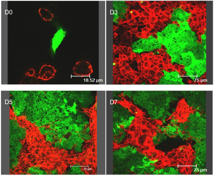
A similar model has been successfully used in our recent work [24] to describe the motion of cancer cells in a Petri dish in the context of cell co-culture experiments of Pasquier et al. [42]. Pasquier et al. [42] cultivated two types of breast cancer cells to study the transfer of proteins between them in a study of multi-drug resistance. It was observed that the two types of cancer cells form segregated clusters of cells of each kind after a 7-day co-culture experiment (Figure 1 (a)). In [24], the authors studied the segregation property of a model similar to (1.1)–(1.2), set in a circular domain in two spatial dimensions x∈ℝ2x\in\mathbb{R}^{2} representing a Petri dish. Starting from islet-like initial conditions representing cell clusters, it was numerically observed that the distribution of cells converges to a segregated state in the long run.

One may observe that in such an experiment the cells are well fed. So there is no limitation for food. As explained in [17], the limitations are due to space and the contact inhibition of growth is involved. Therefore the right hand side of the 1.1 which is a logistic term (for simplicity) could possibly have the following

f⁡(x)=β​x1+α​x−μ​xf(x)=\dfrac{\beta x}{1+\alpha x}-\mu x

where β\beta is the division rate and μ\mu is the mortality rate. We believe that our result hold for such a non-linearity and this is left for future work.

(a)
Refer to caption

(b)

Refer to caption
Figure 1: [24, Figure 1 and Figure 5 (b)]. (a) Direct immunodetection of P-gp transfers in co-cultures of sensitive (MCF-7) and resistant (MCF-7/Doxo) variants of the human breast cancer cell line. (b) The temporal-spatial evolution of the two species in the 1D model. One can check that a discontinuity is forming near the front face of the green surface.

Strikingly, even before the two species come in contact, a sharp transition is formed between the space occupied by one species and the empty space being invaded (Figure 1 (b)) and the distribution of cells looks like a very sharp traveling front. In an attempt to better understand the spatial behavior of cell populations growing in a Petri dish, in the present paper we investigate the mathematical properties of a simplified model for a single species on the real line. We are particularly interested in showing the existence of a sharp traveling front moving at a constant speed.

Recall that a traveling wave a special solution having the specific form

u⁡(t,x)=U⁡(x−c​t), for a.e. ​(t,x)∈ℝ2,u(t,x)=U(x-ct),\text{ for a.e. }(t,x)\in\mathbb{R}^{2},

where the profile UU has the following behavior at ±∞\pm\infty:

limz→−∞U⁡(z)=1,limz→∞U⁡(z)=0.\lim_{z\to-\infty}U(z)=1,\quad\lim_{z\to\infty}U(z)=0.

The goal of this article is to investigate the sharp traveling namely

U⁡(x)=0,∀x>0.U(x)=0,\forall x>0.

Moreover as it is represented in Figure 2-(a) we will obtain the existence of such a wave with a discontinuity at x=0x=0 for the profile UU.

discontinuoustraveling wave(a)smoothtraveling wave(b)
Figure 2: An illustration of two types of traveling wave solutions.

It can be noticed that, in the limit of slow diffusivity σ→0\sigma\to 0 (and under the simplifying assumption that χ=1\chi=1), we get u⁡(t,x)≡p⁡(t,x)u(t,x)\equiv p(t,x) and (1.1) is equivalent to an equation with porous medium-type diffusion and logistic reaction

ut−12​(u2)x​x=u⁡(1−u).u_{t}-\frac{1}{2}(u^{2})_{xx}=u(1-u). (1.3)

We refer to the monograph of Vázquez [46] for more result about porous medium equation.

The propagation dynamics for this kind of equation was first studied, to the extent of our knowledge, by Aronson [2], Atkinson, Reuter and Ridler-Rowe [3], and later by de Pablo and Vázquez [15], in the more general context of nonlinear diffusion

ut=(um)x​x+u⁡(1−u), with ​m>1.u_{t}=(u^{m})_{xx}+u(1-u),\text{ with }m>1. (1.4)

In Section 3.3, we observe that the discontinuous sharp traveling obtained in the present article converge (numerically) to the continuous profile described by Pablo and Vázquez [15].

Our model can be included in the family of non-local advection models for cell-cell adhesion and repulsion. As pointed out by many biologists, cell-cell interactions do not only exist in a local scope, but a long-range interaction should be taken into account to guide the mathematical modeling. Armstrong, Painter and Sherratt [1] in their early work proposed a model (APS model) in which a local diffusion is added to the non-local attraction driven by the adhesion forces to describe the phenomenon of cell mixing, full/partial engulfment and complete sorting in the cell sorting problem. Based on the APS model, Murakawa and Togashi [40] thought that the population pressure should come from the cell volume size instead of the linear diffusion. Therefore, the linear diffusion was changed into a nonlinear diffusion in order to capture the sharp fronts and the segregation in cell co-culture. Carrillo et al. [10] recently proposed a new assumption on the adhesion velocity field and their model showed a good agreement in the experiments in the work of Katsunuma et al. [31]. The idea of the long-range attraction and short-range repulsion can also be seen in the work of Leverentz, Topaz and Bernoff [35]. They considered a non-local advection model to study the asymptotic behavior of the solution. By choosing a Morse-type kernel which follows the attractive-repulsive interactions, they found that the solution can asymptotically spread, contract (blow-up), or reach a steady-state. Burger, Fetecau and Huang [7] considered a similar non-local adhesion model with nonlinear diffusion, for which they investigated the well-posedness and proved the existence of a compactly supported, non-constant steady state. Dyson et al. [21] established the local existence of a classical solution for a non-local cell-cell adhesion model in spaces of uniformly continuous functions. For Turing and Turing-Hopf bifurcation due to the non-local effect, we refer to Ducrot et al. [16] and Song et al. [45]. We also refer to Mogliner et al. [38], Eftimie et al. [22], Ducrot and Magal [18], Ducrot and Manceau [19] for more topics on non-local advection equations. For the derivation of such models, we refer to the work of Bellomo et al. [5] and Morale, Capasso and Oelschläger [39].

Discontinuous traveling waves in hyperbolic partial differential equations have appeared in the literature of the recent few years. Travelling wave solutions with a shock or jump discontinuity have been found e.g. in models of malignant tumor cells (Marchant, Norbury and Perumpanani [36], Harley et al. [28] where the existence of discontinuous waves is proved by means of geometric singular perturbation theory for ODEs) or chemotaxis (Landman, Pettet and Newgreen [34] where both smooth and discontinuous traveling waves are found using phase plane analysis). Bouin, Calvez and Nadin [6] considered the following hyperbolic model

ε2​∂t​tρε+(1−ε2​F′​(ρε))​∂tρε−∂x​xρ⁡(t,x)=F⁡(ρε),\varepsilon^{2}\partial_{tt}\rho_{\varepsilon}+(1-\varepsilon^{2}F^{\prime}(\rho_{\varepsilon}))\partial_{t}\rho_{\varepsilon}-\partial_{xx}\rho(t,x)=F(\rho_{\varepsilon}),

where the reaction term FF is monostable. They identified two different regimes for the propagating behavior of solutions. In the first regime ε2​F​’​(0)<1\varepsilon^{2}F\textquoteright(0)<1, there exists a smooth traveling front (as in the Fisher-KPP case), whereas in the second regime ε2​F​’​(0)>1\varepsilon^{2}F\textquoteright(0)>1 the traveling wave is discontinuous. In the critical case when ε2​F′​(0)=1\varepsilon^{2}F^{\prime}(0)=1, there exists a continuous traveling front with minimal speed F′​(0)\sqrt{F^{\prime}(0)} which may present a jump in the derivative.

The particular relation between the pressure p⁡(t,x)p(t,x) and the density u⁡(t,x)u(t,x) in (1.2) strongly reminds the celebrated model of chemotaxis studied by Patlak (1953) and Keller and Segel (1970) [43, 32, 33] (parabolic-parabolic Keller-Segel model) and, more specifically, the parabolic-elliptic Keller-Segel model which is derived from the former by a quasi-stationary assumption on the diffusion of the chemical [30]. Indeed Equation (1.2) can be formally obtained as the quasistatic approximation of the following parabolic equation

ε​∂tp⁡(t,x)=χ​px​x​(t,x)+u⁡(t,x)−p⁡(t,x),\varepsilon\partial_{t}p(t,x)=\chi p_{xx}(t,x)+u(t,x)-p(t,x),

when ε→0\varepsilon\to 0. A rigorous derivation of the limit has been achieved in the case of the Keller-Segel model by Carrapatoso and Mischler [9]. We also refer to Mottoni and Rothe [14] for such a result in the context of linear parabolic equations. We refer to [8, 29, 44] and the references therein for a mathematical introduction and biological applications. In these models, the field p⁡(t,x)p(t,x) is interpreted as the concentration of a chemical produced by the cells rather than a physical pressure. One of the difficulties in attractive chemotaxis models is that two opposite forces compete to drive the behavior of the equations: the diffusion due to the random motion of cells, on the one hand, and on the other hand the non-local advection due to the attractive chemotaxis; the former tends to regularize and homogenize the solution, while the latter promotes cell aggregation and may lead to the blow-up of the solution in finite time [12, 30]. At this point let us mention that our study concerns repulsive cell-cell interaction with no diffusion, therefore no such blow-up phenomenon is expected in our study; however the absence of diffusion adds to the mathematical complexity of the study, because standard methods of reaction-diffusion equations cannot be employed here. Traveling waves for the (attractive) parabolic-elliptic Keller-Segel model were studied by Nadin, Perthame and Ryzhik [41], who constructed these traveling wave by a bounded interval approximation of the 1D system

{ut+χ​(u​px)x=ux​x+u⁡(1−u),−d​px​x+p=u,\left\{\begin{array}[]{l}u_{t}+\chi\,(up_{x})_{x}=u_{xx}+u(1-u),\\ -d\,p_{xx}+p=u,\end{array}\right. (1.5)

set on the real line x∈ℝx\in\mathbb{R}, when the strength of the advection is not too strong 0<χ<min⁡(1,d)0<\chi<\min(1,d), and gave estimates on the speed of such a traveling wave: 2≤c∗≤2+χ​d/(d−χ)2\leq c_{*}\leq 2+\chi\sqrt{d}/(d-\chi).

Since the pressure p⁡(t,x)p(t,x) is a non-local function of the density u⁡(t,x)u(t,x) in (1.2), the spatial derivative appears as a non-local advection term in (1.1). In fact, our problem (1.1)–(1.2) can be rewritten as a transport equation in which the speed of particles is non-local in the density,

{∂tu⁡(t,x)−χ​∂x(u⁡(t,x)​∂x(ρ⋆u)​(t,x))=u⁡(t,x)​(1−u⁡(t,x))u⁡(t=0,x)=u0​(x),\left\{\begin{array}[]{l}\partial_{t}u(t,x)-\chi\partial_{x}(u(t,x)\partial_{x}(\rho\star u)(t,x))=u(t,x)(1-u(t,x))\\ u(t=0,x)=u_{0}(x),\end{array}\right. (1.6)

where

(ρ⋆u)​(x)=∫ℝρ⁡(x−y)​u​(t,y)​𝑑y,ρ⁡(x)=12​σ​e−|x|σ.\left(\rho\star u\right)(x)=\int_{\mathbb{R}}\rho(x-y)u(t,y)dy,\quad\rho(x)=\frac{1}{2\sigma}e^{-\frac{|x|}{\sigma}}. (1.7)

Traveling waves for a similar diffusive equation with logistic reaction have been investigated for quite general non-local kernels by Hamel and Henderson [27], who considered the model

ut+(u⁡(K⋆u))x=ux​x+u⁡(1−u),u_{t}+(u\,(K\star u))_{x}=u_{xx}+u(1-u), (1.8)

where K∈Lp​(ℝ)K\in L^{p}(\mathbb{R}) is odd and p∈[1,∞]p\in[1,\infty]. Notice that the attractive parabolic-elliptic Keller-Segel model (1.5) is included in this framework by the particular choice

K(x)=−χsign(x)e−|x|/d/(2d).K(x)=-\chi\,{\rm sign}(x)e^{-|x|/\sqrt{d}}/\big(2\sqrt{d}\big).

They proved a spreading result for this equation (initially compactly supported solutions to the Cauchy problem propagate to the whole space with constant speed) and explicit bounds on the speed of propagation. Diffusive non-local advection also appears in the context of swarm formation [37]. Pattern formation for a model similar to (1.8) by Ducrot, Fu and Magal [16]. Let us mention that the inviscid equation (1.6) has been studied in a periodic cell by Ducrot and Magal [18]. Other methods have been established for conservative systems of interacting particles and their kinetic limit (Balagué et al. [4], Carrillo et al. [11]) based on gradient flows set on measure spaces; those are difficult to adapt here because of the logistic term. Finally we refer to [13, 26, 47, 23, 20] for other examples of traveling waves in non-local reaction-diffusion equations.

In this paper we focus on the particular case of (1.1)–(1.2) with σ>0\sigma>0 and χ>0\chi>0. The paper is organized as follows. In Section 2, we present our main results. In Section 3 we present numerical simulations to illustrate our theoretical results. In Section 4, we prove the propagation properties of the solution and describe the local behavior near the propagating boundary (see Proposition 2.4 for definition), including the formation of a discontinuity for time-dependent solutions. In Section 5 we prove the existence of sharp traveling waves. We also prove that smooth traveling waves are necessarily positive, which shows that sharp traveling waves are necessarily singular (in this case, discontinuous). In particular, a solution starting from a compactly supported initial condition with polynomial behavior at the boundary can never catch such a smooth traveling wave.

2 Main results and comments

We begin by defining our notion of solution to equation (1.1).

Definition 2.1 (Integrated solutions).

Let u0∈L∞​(ℝ)u_{0}\in L^{\infty}(\mathbb{R}). A measurable function u⁡(t,x)∈L∞​([0,T]×ℝ)u(t,x)\in L^{\infty}([0,T]\times\mathbb{R}) is an integrated solution to (1.1) if the characteristic equation

{dd​t​h​(t,x)=−χ⁡(ρx⋆u)​(t,h⁡(t,x))h⁡(t=0,x)=x.\left\{\begin{array}[]{l}\frac{\mathrm{d}\phantom{t}}{\mathrm{d}t}h(t,x)=-\chi(\rho_{x}\star u)(t,h(t,x))\\ h(t=0,x)=x.\end{array}\right. (2.1)

has a classical solution h⁡(t,x)h(t,x) (i.e. for each x∈ℝx\in\mathbb{R} fixed, the function t↦h⁡(t,x)t\mapsto h(t,x) is in C1​([0,T],ℝ)C^{1}([0,T],\mathbb{R}) and satisfies (2.1)), and for a.e. x∈ℝx\in\mathbb{R}, the function t↦u⁡(t,h⁡(t,x))t\mapsto u(t,h(t,x)) is in C1​([0,T],ℝ)C^{1}([0,T],\mathbb{R}) and satisfies

{dd​t​u​(t,h⁡(t,x))=u⁡(t,h⁡(t,x))​(1+χ^​(ρ⋆u)​(t,h⁡(t,x))−(1+χ^)​u​(t,h⁡(t,x))),u⁡(t=0,x)=u0​(x),\left\{\begin{array}[]{l}\frac{\mathrm{d}\phantom{t}}{\mathrm{d}t}u(t,h(t,x))=u(t,h(t,x))\big(1+\hat{\chi}(\rho\star u)(t,h(t,x))-(1+\hat{\chi})u(t,h(t,x))\big),\\ u(t=0,x)=u_{0}(x),\end{array}\right. (2.2)

where χ^:=χσ2\hat{\chi}:=\frac{\chi}{\sigma^{2}}.

We define weighted space Lη1​(ℝ)L^{1}_{\eta}(\mathbb{R}) as follows

Lη1(ℝ):={f:ℝ→ℝ measurable|∫ℝ|f(x)|e−η​|x|dx<∞}.L^{1}_{\eta}(\mathbb{R}):=\bigg\{f:\mathbb{R}\to\mathbb{R}\text{ measurable}\,\bigg|\int_{\mathbb{R}}|f(x)|e^{-\eta|x|}\mathrm{d}x<\infty\bigg\}.

Lη1​(ℝ)L^{1}_{\eta}(\mathbb{R}) is a Banach space endowed with the norm

‖f‖Lη1:=η2​∫ℝ|f⁡(y)|​e−η​|y|​𝑑y.\|f\|_{L^{1}_{\eta}}:=\frac{\eta}{2}\int_{\mathbb{R}}|f(y)|e^{-\eta|y|}\mathrm{d}y.

We first recall some results concerning the existence of integrated solutions for equation (1.1) in Theorem 2.1, Proposition 2.2 and Theorem 2.3. We prove those results in the companion paper [25].

Theorem 2.1 (Well-posedness ).

Let u0∈L+∞​(ℝ)u_{0}\in L^{\infty}_{+}(\mathbb{R}) and fix η>0\eta>0. There exists τ∗(u0)∈(0,+∞]\tau^{*}(u_{0})\in(0,+\infty] such that for all τ∈(0,τ∗​(u0))\tau\in(0,\tau^{*}(u_{0})), there exists a unique integrated solution u∈C0​([0,τ],Lη1​(ℝ))u\in C^{0}([0,\tau],L^{1}_{\eta}(\mathbb{R})) to (1.1) which satisfies u⁡(t=0,x)=u0​(x)u(t=0,x)=u_{0}(x). Moreover u⁡(t,⋅)∈L∞​(ℝ)u(t,\cdot)\in L^{\infty}(\mathbb{R}) for each t∈[0,τ∗​(u0))t\in[0,\tau^{*}(u_{0})) and the map t∈[0,τ∗​(u0))↦Tt​u0:=u⁡(t,⋅)t\in[0,\tau^{*}(u_{0}))\mapsto T_{t}u_{0}:=u(t,\cdot) is a semigroup which is continuous for the Lη1​(ℝ)L^{1}_{\eta}(\mathbb{R})-topology. The map u0∈L∞​(ℝ)↦Tt​u0∈Lη1​(ℝ)u_{0}\in L^{\infty}(\mathbb{R})\mapsto T_{t}u_{0}\in L^{1}_{\eta}(\mathbb{R}) is continuous.

Finally, if 0≤u0​(x)≤10\leq u_{0}(x)\leq 1, then τ∗​(u0)=+∞\tau^{*}(u_{0})=+\infty and 0≤u⁡(t,⋅)≤10\leq u(t,\cdot)\leq 1 for all t>0t>0.

The next result concerns the preservation properties satisfied by the solutions of (1.1) (see [25, Proposition 2.2]).

Proposition 2.2 (Regularity of solutions).

Let u⁡(t,x)u(t,x) be an integrated solution to (1.1).

  1. 1.

    if u0​(x)u_{0}(x) is continuous, then u⁡(t,x)u(t,x) is continuous for each t>0t>0.

  2. 2.

    if u0​(x)u_{0}(x) is monotone, then u⁡(t,x)u(t,x) has the same monotony for each t>0t>0.

  3. 3.

    if u0​(x)∈C1​(ℝ)u_{0}(x)\in C^{1}(\mathbb{R}), then u∈C1​([0,T]×ℝ)u\in C^{1}([0,T]\times\mathbb{R}) and uu is then a classical solution to (1.1).

In this following theorem we consider the long-time behavior of some solutions to (1.1) (see [25, Theorem 2.3]).

Theorem 2.3 (Long-time behavior).

Let 0≤u0​(x)≤10\leq u_{0}(x)\leq 1 be a nontrivial non-negative initial condition and u⁡(t,x)u(t,x) be the corresponding integrated solution. Then 0≤u⁡(t,x)≤10\leq u(t,x)\leq 1 for all t>0t>0 and x∈ℝx\in\mathbb{R}. If moreover there exists δ>0\delta>0 such that δ≤u0​(x)≤1\delta\leq u_{0}(x)\leq 1 then

u⁡(t,x)→1, as ​t→∞u(t,x)\to 1,\text{ as }t\to\infty

and the convergence holds uniformly in x∈ℝx\in\mathbb{R}.

We now arrive at the main interest of the paper, which is to describe the spatial dynamics of solutions to (1.1)–(1.2). To get insight about the asymptotic propagation properties of the solutions, we focus on initial conditions whose support is bounded towards +∞+\infty. If the behavior of the initial condition in a neighbourhood of the boundary of the support is polynomial, we can establish a precise estimate of the location of the level sets relative to the position of the rightmost positive point. Our first assumption requires that the initial condition is supported in (−∞,0](-\infty,0].

Assumption 1 (Initial condition).

We assume that u0​(x)u_{0}(x) is a continuous function satisfying

0≤u0​(x)\displaystyle 0\leq u_{0}(x) ≤1,\displaystyle\leq 1, ∀x∈ℝ,\displaystyle\forall x\in\mathbb{R},
u0​(x)\displaystyle u_{0}(x) =0,\displaystyle=0, ∀x≥0,\displaystyle\forall x\geq 0,
u0​(x)\displaystyle u_{0}(x) >0,\displaystyle>0, ∀x∈(−δ0,0),\displaystyle\forall x\in(-\delta_{0},0),

for some δ0>0\delta_{0}>0.

Under this assumption we show that uu is propagating to the right.

Proposition 2.4 (The separatrix).

Let u0​(x)u_{0}(x) satisfy Assumption 1, and h∗​(t):=h⁡(t,0)h^{*}(t):=h(t,0) be the separatrix. Then h∗​(t)h^{*}(t) stays at the rightmost boundary of the support of u⁡(t,⋅)u(t,\cdot), i.e.

  1. (i)

    we have

    u⁡(t,x)=0​ for all ​x≥h∗​(t),\qquad u(t,x)=0\text{ for all }x\geq h^{*}(t), (2.3)
  2. (ii)

    for each t>0t>0 there exists δ>0\delta>0 such that

    u⁡(t,x)>0​ for all ​x∈(h∗​(t)−δ,h∗​(t)).\qquad u(t,x)>0\text{ for all }x\in\big(h^{*}(t)-\delta,h^{*}(t)\big). (2.4)

Moreover, uu is propagating to the right i.e.

dd​t​h∗​(t)>0​ for all ​t>0.\qquad\frac{\mathrm{d}\phantom{t}}{\mathrm{d}t}h^{*}(t)>0\text{ for all }t>0.

We precise the behavior of the initial condition in a neighbourhood of 00 and estimate the steepness of uu in positive time.

Assumption 2 (Polynomial behavior near 0).

In addition to Assumption 1, we require that there exists α≥1\alpha\geq 1 and γ>0\gamma>0 such that

u0​(x)≥γ​|x|α,∀x∈(−δ,0).u_{0}(x)\geq\gamma|x|^{\alpha},\qquad\forall x\in(-\delta,0).
Theorem 2.5 (Formation of a discontinuity).

Let u0​(x)u_{0}(x) satisfy Assumptions 1 and 2 and u⁡(t,x)u(t,x) solve (1.1) with u⁡(t=0,x)=u0​(x)u(t=0,x)=u_{0}(x). For all δ>0\delta>0 we have

lim supt→+∞supx∈(h∗​(t)−δ,h∗​(t))u⁡(t,x)≥11+χ^+α​χ>0.\limsup_{t\to+\infty}\sup_{x\in(h^{*}(t)-\delta,h^{*}(t))}u(t,x)\geq\frac{1}{1+\hat{\chi}+\alpha\chi}>0. (2.5)

More precisely, define the level set

ξ⁡(t,β):=sup{x∈ℝ|u⁡(t,x)=β},\xi(t,\beta):=\sup\{x\in\mathbb{R}\,|\,u(t,x)=\beta\},

for all t>0t>0 and 0<β<11+χ^+α​χ0<\beta<\frac{1}{1+\hat{\chi}+\alpha\chi}. Then, for each 0<β<11+χ^+α​χ0<\beta<\frac{1}{1+\hat{\chi}+\alpha\chi}, the distance between ξ⁡(t,β)\xi(t,\beta) and the separatrix is decaying exponentially fast:

h∗​(t)−(βγ)1α​e−η2​α​t≤ξ⁡(t,β)≤h∗​(t),h^{*}(t)-\left(\frac{\beta}{\gamma}\right)^{\frac{1}{\alpha}}e^{-\frac{\eta}{2\alpha}t}\leq\xi(t,\beta)\leq h^{*}(t), (2.6)

where η∈(0,1)\eta\in(0,1) is given in Proposition 4.5 and χ^=χσ2\hat{\chi}=\frac{\chi}{\sigma^{2}}.

h∗​(t1)h^{*}(t_{1})h∗​(t2)h^{*}(t_{2})β\betaξ⁡(t1,β)\xi(t_{1},\beta)t=t1t=t_{1}ξ⁡(t2,β)\xi(t_{2},\beta)t=t2t=t_{2}
Figure 3: A cartoon for the formation of the discontinuity. Here we choose t1<t2t_{1}<t_{2} and ξ⁡(t,β),t=t1,t2\xi(t,\beta),t=t_{1},t_{2} are the level sets. Theorem 2.5 proves that when Assumptions 1 and 2 are satisfied, then the distance |ξ⁡(t,β)−h∗​(t)||\xi(t,\beta)-h^{*}(t)| converges to 0 exponentially fast.

In particular, the profile u⁡(t,x)u(t,x) forms a discontinuity near the boundary point h∗​(t)h^{*}(t) as t→+∞t\to+\infty. By considering discontinuous integrated solutions, we are able to estimate the size of the jump for non increasing profiles, which leads to an estimate of the asymptotic speed.

Proposition 2.6 (Asymptotic jump near the separatrix).

Let u0u_{0} be a non increasing function satisfying u0​(−∞)≤1u_{0}(-\infty)\leq 1, u0​(0)>0u_{0}(0)>0 and u0​(x)=0u_{0}(x)=0 for x>0x>0. Then

lim inft→+∞u⁡(t,h∗​(t))\displaystyle\liminf_{t\to+\infty}u(t,h^{*}(t)) ≥22+χ^,\displaystyle\geq\frac{2}{2+\hat{\chi}}, (2.7)
lim inft→+∞dd​t​h∗​(t)\displaystyle\liminf_{t\to+\infty}\frac{\mathrm{d}}{\mathrm{d}t}h^{*}(t) ≥σ​χ^2+χ^,\displaystyle\geq\frac{\sigma\hat{\chi}}{2+\hat{\chi}}, (2.8)

where χ^=χσ2\hat{\chi}=\frac{\chi}{\sigma^{2}}.

We finally turn to traveling wave solutions u⁡(t,x)=U⁡(x−c​t)u(t,x)=U(x-ct), which are self-similar profiles traveling at a constant speed.

Definition 2.2 (Traveling wave solution).

A traveling wave is a positive solution u⁡(t,x)u(t,x) to (1.1) such that there exists a function U∈L∞​(ℝ)U\in L^{\infty}(\mathbb{R}) and a speed c∈ℝc\in\mathbb{R} such that u⁡(t,x)=U⁡(x−c​t)u(t,x)=U(x-ct) for a.e. (t,x)∈ℝ2(t,x)\in\mathbb{R}^{2}. By convention, we also require that UU has the following behavior at ±∞\pm\infty:

limz→−∞U⁡(z)=1,limz→∞U⁡(z)=0.\lim_{z\to-\infty}U(z)=1,\quad\lim_{z\to\infty}U(z)=0.

The function UU is the profile of the traveling wave.

Under a technical assumption on χ^=χσ2\hat{\chi}=\frac{\chi}{\sigma^{2}}, we can prove the existence of sharp traveling waves which present a jump at the vanishing point.

Assumption 3 (Bounds on χ^\hat{\chi}).

Let χ>0\chi>0 and σ>0\sigma>0 be given and define χ^:=χσ2\hat{\chi}:=\frac{\chi}{\sigma^{2}}. We assume that 0<χ^<χ¯0<\hat{\chi}<\bar{\chi}, where χ¯\bar{\chi} is the unique root of the function

χ^↦ln⁡(2−χ^χ^)+22+χ^​(χ^2​ln⁡(χ^2)+1−χ^2)\hat{\chi}\mapsto\ln\left(\frac{2-\hat{\chi}}{\hat{\chi}}\right)+\frac{2}{2+\hat{\chi}}\left(\frac{\hat{\chi}}{2}\ln\left(\frac{\hat{\chi}}{2}\right)+1-\frac{\hat{\chi}}{2}\right)

given by Lemma A.1.

Remark 2.1.

It follows from Lemma A.1 that χ^=1\hat{\chi}=1 satisfies Assumption 3. Actually, numerical evidence suggest that χ¯≈1.045\bar{\chi}\approx 1.045.

Theorem 2.7 (Existence of a sharp discontinuous traveling wave).

Let Assumption 3 be satisfied. There exists a traveling wave u⁡(t,x)=U⁡(x−c​t)u(t,x)=U(x-ct) traveling at speed

c∈(σ​χ^2+χ^,σ​χ^2),c\in\left(\frac{\sigma\hat{\chi}}{2+\hat{\chi}},\frac{\sigma\hat{\chi}}{2}\right),

where χ^=χσ2\hat{\chi}=\frac{\chi}{\sigma^{2}}

Moreover, the profile UU satisfies the following properties (up to a shift in space):

  1. (i)

    UU is sharp in the sense that U⁡(x)=0U(x)=0 for all x≥0x\geq 0; moreover, UU has a discontinuity at x=0x=0 with U⁡(0−)≥22+χ^U(0^{-})\geq\frac{2}{2+\hat{\chi}}.

  2. (ii)

    UU is continuously differentiable and strictly decreasing on (−∞,0](-\infty,0], and satisfies

    −c​U′−χ​(U​P′)′=U⁡(1−U)-c\,U^{\prime}-\chi(UP^{\prime})^{\prime}=U(1-U)

    pointwise on (−∞,0)(-\infty,0), where P​(z):=(ρ⋆U)​(z)P(z):=(\rho\star U)(z).

Finally, we show that continuous traveling waves cannot be sharp, i.e. are necessarily positive on ℝ\mathbb{R}.

Proposition 2.8 (Smooth traveling waves).

Let U⁡(x)U(x) be the profile of a traveling wave solution to (1.1) and assume that UU is continuous. Then U∈C1​(ℝ)U\in C^{1}(\mathbb{R}), UU is strictly positive and we have the estimate:

−χ⁡(ρx⋆U)​(x)<c​ for all ​x∈ℝ.-\chi(\rho_{x}\star U)(x)<c\text{ for all }x\in\mathbb{R}. (2.9)

In particular, by Theorem 2.5, any solutions starting from an initial condition satisfying Assumption 2 may never catch such a traveling wave.

3 Numerical Simulations

We first describe the numerical framework of this study.

  • •

    The parameters σ\sigma and χ\chi are fixed to 1, σ=1\sigma=1 and χ=1\chi=1.

  • •

    We are given a bounded interval [−L,L][-L,L] and an initial distribution of ϕ∈C⁡([−L,L])\phi\in C([-L,L]);

  • •

    We solve numerically the following PDE using the upwind scheme (pp being given)

    {∂tu⁡(t,x)−∂x(u⁡(t,x)​∂xp⁡(t,x))=u⁡(t,x)​(1−u⁡(t,x)),∇p​(t,x)⋅ν=0u⁡(0,x)=ϕ⁡(x),​t>0,x∈[−L,L].\begin{cases}\partial_{t}u(t,x)-\partial_{x}\bigl(u(t,x)\partial_{x}p(t,x)\bigr)=u(t,x)(1-u(t,x)),\\ \nabla p(t,x)\cdot\nu=0\\ u(0,x)=\phi(x),\end{cases}\;\;t>0,\;x\in[-L,L]. (3.1)
  • •

    The pressure pp is defined as

    p(t,x)=(I−Δ)𝒩−1u(t,x),t>0,x∈[−L,L],\displaystyle p(t,x)=(I-\Delta)_{\mathcal{N}}^{-1}u(t,x),\quad t>0,x\in[-L,L], (3.2)

    where (I−Δ)𝒩−1(I-\Delta)_{\mathcal{N}}^{-1} is the Laplacian operator with Neumann boundary condition. Due to the Neumann boundary condition of the pressure pp, we do not need boundary condition on uu (see [41, 24]).

Our numerical scheme reads as follows

uin+1−uinΔ​t+1Δ​x​(G⁡(ui+1n,uin)−G⁡(uin,ui−1n))=uin​(1−uin),\displaystyle\frac{u^{n+1}_{i}-u^{n}_{i}}{\Delta t}+\,\frac{1}{\Delta x}\bigg(G(u_{i+1}^{n},u_{i}^{n})-G(u_{i}^{n},u_{i-1}^{n})\bigg)=u_{i}^{n}(1-u_{i}^{n}),
i=1,2,…,M,n=0,1,2,…\displaystyle i=1,2,\ldots,M,\ n=0,1,2,\ldots
u0=1,uM+1=0,\displaystyle u_{0}=1,\;u_{M+1}=0,

with G⁡(ui+1n,uin)G(u_{i+1}^{n},u_{i}^{n}) defined as

G⁡(ui+1n,uin)=(vi+12n)+​uin−(vi+12n)−​ui+1n={vi+12n​uin,vi+12n≥0,vi+12n​ui+1n,vi+12n<0,i=1,…,M.G(u_{i+1}^{n},u_{i}^{n})=(v_{i+\frac{1}{2}}^{n})^{+}u_{i}^{n}-(v_{i+\frac{1}{2}}^{n})^{-}u_{i+1}^{n}=\begin{cases}v_{i+\frac{1}{2}}^{n}u_{i}^{n},&v_{i+\frac{1}{2}}^{n}\geq 0,\\ v_{i+\frac{1}{2}}^{n}u_{i+1}^{n},&v_{i+\frac{1}{2}}^{n}<0,\end{cases}\quad i=1,\ldots,M.

Moreover the velocity vv is given by

vi+12n=−pi+1n−pinΔ​x,i=0,1,2,⋯,M,v_{i+\frac{1}{2}}^{n}=-\dfrac{p_{i+1}^{n}-p_{i}^{n}}{\Delta x},\ i=0,1,2,\cdots,M,

where from (3.2) we define

Pn:=(I−A)−1​Un,Pn=(pin)M×1Un=(uin)M×1.P^{n}:=(I-A)^{-1}U^{n},\quad P^{n}=\big(p_{i}^{n}\big)_{M\times 1}\quad U^{n}=\big(u_{i}^{n}\big)_{M\times 1}.

where A=(ai,j)M×MA=(a_{i,j})_{M\times M} is the usual linear diffusion matrix with Neumann boundary condition. Therefore, by Neumann boundary condition p0=p1p_{0}=p_{1} and pM+1=pMp_{M+1}=p_{M}, when i=1,Mi=1,M we have

G⁡(u1n,u0n)=0,\displaystyle G(u_{1}^{n},u_{0}^{n})=0,
G⁡(uM+1n,uMn)=0,\displaystyle G(u_{M+1}^{n},u_{M}^{n})=0,

which gives

u1n+1\displaystyle u^{n+1}_{1} =u1n−d​Δ​tΔ​x​G​(u2n,u1n)+Δ​t​f​(u1n),\displaystyle=u^{n}_{1}-d\,\frac{\Delta t}{\Delta x}G(u_{2}^{n},u_{1}^{n})+\Delta t\,f(u_{1}^{n}),
uMn+1\displaystyle u^{n+1}_{M} =uMn+d​Δ​tΔ​x​G​(uMn,uM−1n)+Δ​t​f​(uMn).\displaystyle=u^{n}_{M}+d\,\frac{\Delta t}{\Delta x}G(u_{M}^{n},u_{M-1}^{n})+\Delta t\,f(u_{M}^{n}).

Owing to the boundary condition, we have the conservation of mass for Equation (3.1) when the reaction term equals zero.

3.1 Formation of a discontinuity

In this part, we use numerical simulations to verify the theoretical predictions in the previous sections. Firstly, we choose the initial value ϕ∈C1​([−L,L])\phi\in C^{1}([-L,L]) as follows

ϕ⁡(x)=(x−x0)2(L+x0)2​𝟙[−L,x0]​(x),L=20,x0=−15.\phi(x)=\frac{(x-x_{0})^{2}}{(L+x_{0})^{2}}\mathbbm{1}_{[-L,x_{0}]}(x),\quad L=20,\;x_{0}=-15. (3.3)

Notice that this initial condition satisfies Assumptions 1 and 2. Due to Theorem 2.5, we should observe the formation of a discontinuity in space for large time.

We plot the evolution of the solution u⁡(t,x)u(t,x) starting from u⁡(0,x)=ϕ⁡(x)u(0,x)=\phi(x) in Figure 4.

Figure 4: We plot the propagation of the traveling waves under system (3.1) with the initial value (3.3). We plot the propagation profile at t=0,10,25,40t=0,10,25,40 (resp. dashed lines, dotted-dashed lines, dotted lines and solid lines).

We observe that the jump is formed for large time and the height of the jump is greater than 2/32/3 which is in accordance with Theorem 2.7.

Next, we study the propagation speed of different level sets, namely,

t⟼ξ⁡(t,β)+L,t\longmapsto\xi(t,\beta)+L,

where ξ⁡(t,β):=sup{x∈ℝ|u⁡(t,x)=β}\xi(t,\beta):=\sup\{x\in\mathbb{R}\,|\,u(t,x)=\beta\} and β=0,0.2,2/3,0.8\beta=0,0.2,2/3,0.8. Note that the case β=0\beta=0 corresponds to the rightmost characteristic.

We compute the propagation speed in the following way: for different β∈[0,1]\beta\in[0,1], we choose t1=15t_{1}=15 and t2=40t_{2}=40 where the propagation speed is almost stable after t=t1t=t_{1}. Thus we can compute the mean propagation speed as follows

Propagation speed at level β=ξ⁡(t2,β)−ξ⁡(t1,β)t2−t1.\text{Propagation speed at level $\beta$}=\frac{\xi(t_{2},\beta)-\xi(t_{1},\beta)}{t_{2}-t_{1}}. (3.4)
Figure 5: We plot the evolution of different level sets t⟼ξ⁡(t,β)+Lt\longmapsto\xi(t,\beta)+L under system (3.1). Our initial distribution is taken as (3.3). We plot the propagating speeds of the profile at β=0,0.2,2/3,0.8\beta=0,0.2,2/3,0.8. The x-axis represents the time and the y-axis is the relative distance ξ⁡(t,β)+L\xi(t,\beta)+L. The velocity is calculated by (3.4) for t1=15t_{1}=15 and t2=40t_{2}=40.

Next we want to check whether the solutions of system (3.2) starting from two different initial values converge to the same discontinuous traveling wave solution. To that aim, given two different initial profiles ϕ1\phi_{1} and ϕ2\phi_{2} with ϕ1≤ϕ2\phi_{1}\leq\phi_{2} on [−L,L][-L,L],

ϕ1​(x)=−x+155​𝟙[−20,−15]​(x),ϕ2​(x)=𝟙[−20,−17.5]​(x)−x+1510​𝟙[−17.5,−15]​(x)\phi_{1}(x)=-\frac{x+15}{5}\mathbbm{1}_{[-20,-15]}(x),\quad\phi_{2}(x)=\mathbbm{1}_{[-20,-17.5]}(x)-\frac{x+15}{10}\mathbbm{1}_{[-17.5,-15]}(x) (3.5)

We simulate the propagation of these two profiles in Figure 6.

Figure 6: We plot the propagation of two profiles under system (3.1) with initial distributions are taken as (3.5). The blue curves represent the profile with initial distribution ϕ1\phi_{1} while the red curves represent the profile with initial distribution ϕ2\phi_{2}. We plot the propagation profiles at t=0,15t=0,15 and 3030 (resp. dashed lines, dotted-dashed lines and solid lines). The simulation shows that the two profiles converge to the same discontinuous traveling wave solution.

3.2 Large speed traveling waves

As we know for porous medium equation, the existence of large speed c>c∗c>c_{*} traveling wave solutions is proved in [15] and it can be observed numerically by taking the exponentially decreasing function as initial value. In this part, instead of taking a compactly supported initial value, we set the initial value

ϕα​(x)=11+eα⁡(x−x0),x0=−15,\phi_{\alpha}(x)=\frac{1}{1+e^{\alpha(x-x_{0})}},\quad x_{0}=-15, (3.6)

where α≥1\alpha\geq 1 is a parameter introduced to describe the decaying rate of the initial value.

We compare the following three different scenarios with different parameters α=1,2,5\alpha=1,2,5 in the initial value (3.6).

Figure 7: We plot the propagation of the traveling waves under system (3.1) with the initial values (3.6) and the corresponding evolution of different level sets t⟼ξ⁡(t,β)+Lt\longmapsto\xi(t,\beta)+L. Figure (a) and (d) represent the evolution of the traveling wave and its level sets when α=1\alpha=1. Figure (b) and (e) correspond to the case when α=2\alpha=2. Figure (c) and (f) correspond to the case when α=5\alpha=5.

We observe the large speed traveling waves in Figure 7 when α=1,2\alpha=1,2. We note that as the parameter α\alpha in (3.6) is increasing, the propagation speed is decreasing and c≈1/αc\approx 1/\alpha. When α=5\alpha=5, the propagation of the traveling waves is similar to the case in Figure 4 in which we started from the compactly supported initial value. In other word, we can observe the formation of discontinuity and the critical speed c∗≈0.414c_{*}\approx 0.414 is reached.

3.3 Comparison with porous medium equations: the vanishing jump

In this part, we compare the non-local advection model with the porous medium equation by introducing a new parameter σ\sigma

p⁡(t,x)=(I−σ2​Δ)𝒩−1​u​(t,x)p(t,x)=(I-\sigma^{2}\Delta)_{\mathcal{N}}^{-1}u(t,x) (3.7)

Thus if σ→0\sigma\to 0 then formally we have p⁡(t,x)→u⁡(t,x)p(t,x)\to u(t,x). Thus, the first equation of (3.1) becomes

ut−12​(u2)x​x=u⁡(1−u),u_{t}-\frac{1}{2}(u^{2})_{xx}=u(1-u),

which is the classical porous medium equation. It is well-known that this equation has the explicit traveling wave solution U⁡(z)=(1−ez/2)+U(z)=(1-e^{z/\sqrt{2}})_{+} with critical speed c∗=1/2c_{*}=1/\sqrt{2}.

We are consider the transition from the discontinuous traveling wave solution to the continuous sharp-type traveling wave solution by letting σ→0\sigma\to 0. Moreover, we want to see if the critical traveling speed of the discontinuous wavefront c⁡(σ)c(\sigma) converges to c∗=1/2≈0.707c_{*}=1/\sqrt{2}\approx 0.707 as σ→0\sigma\to 0. Our initial value is taken as 1/(1+exp⁡(5∗(x+15))),x∈[−20,20]1/(1+{\rm exp}(5*(x+15))),x\in[-20,20] in (3.6). We compare the following three different scenarios with different parameters σ2=0.5,0.1,0.01\sigma^{2}=0.5,0.1,0.01 in kernel (3.7).

Figure 8: We plot the propagation of the traveling waves for system (3.1) with the kernel (3.7) and the corresponding evolution of different level sets t⟼ξ⁡(t,β)+Lt\longmapsto\xi(t,\beta)+L. Figure (a) and (d) represent the evolution of the traveling wave and its level sets when σ2=0.5\sigma^{2}=0.5. Figure (b) and (e) correspond to the case when σ2=0.1\sigma^{2}=0.1. Figure (c) and (f) correspond to the case when σ2=0.01\sigma^{2}=0.01. Our initial value is taken as in (3.6) with α=5\alpha=5.

In Figure 8 we can observe that as σ→0\sigma\to 0 in the kernel, the discontinuous jump is gradually vanishing from (a) to (c). Moreover, the critical speed c⁡(σ)c(\sigma) is increasing as σ→0\sigma\to 0 and is approaching the critical speed c∗=1/2≈0.707c_{*}=1/\sqrt{2}\approx 0.707 for the porous medium case.

4 Properties of the time-dependent solutions

4.1 The separatrix

In this section we study the qualitative properties of solutions to (1.1) starting from an initial condition supported in (−∞,0](-\infty,0].

Proposition 4.1 (The separatrix).

Let uu be a solution integrated along the characteristics to (1.1), starting from u0​(x)u_{0}(x) satisfying Assumption 1. Let h∗​(t):=h⁡(t,0)h^{*}(t):=h(t,0) be the separatrix (as in Proposition 2.4). Then h∗​(t)h^{*}(t) stays at the rightmost boundary of the support of u⁡(t,⋅)u(t,\cdot), i.e.

  1. (i)

    we have

    u⁡(t,x)=0​ for all ​x≥h∗​(t).u(t,x)=0\text{ for all }x\geq h^{*}(t). (4.1)
  2. (ii)

    for each t>0t>0 there exists δ>0\delta>0 such that

    u⁡(t,x)>0​ for all ​x∈(h∗​(t)−δ,h∗​(t)).u(t,x)>0\text{ for all }x\in(h^{*}(t)-\delta,h^{*}(t)). (4.2)
Proof.

By definition the characteristics are well-defined by (2.1) as the flow of an ODE. In particular, if x≥h∗​(t)=h⁡(t,0)x\geq h^{*}(t)=h(t,0) there exists x0≥0x_{0}\geq 0 such that x=h⁡(t,x0)x=h(t,x_{0}). Since u0​(x0)=0u_{0}(x_{0})=0 and in view of (2.2), we have indeed u⁡(t,x)=0u(t,x)=0. This proves Item (i)

By Assumption 1, there exists δ0>0\delta_{0}>0 such that u0​(x)>0u_{0}(x)>0 for x∈(−δ0,0)x\in(-\delta_{0},0). We remark that

dd​t​u​(t,h⁡(t,x))\displaystyle\frac{\mathrm{d}}{\mathrm{d}t}u(t,h(t,x)) =χ^​u​(t,h⁡(t,x))​((ρ∗u)​(t,h⁡(t,x))−u⁡(t,h⁡(t,x)))+u⁡(t,h⁡(t,x))​(1−u⁡(t,h⁡(t,x)))\displaystyle=\hat{\chi}\,u(t,h(t,x))\big((\rho*u)(t,h(t,x))-u(t,h(t,x))\big)+u(t,h(t,x))\big(1-u(t,h(t,x))\big)
≥u⁡(t,h⁡(t,x))​(1−(1+χ^)​u​(t,h⁡(t,x))).\displaystyle\geq u(t,h(t,x))\big(1-(1+\hat{\chi})u(t,h(t,x))\big).

By comparison with the solution to the ODE v′​(t)=v⁡(t)​(1−(1+χ^)​v​(t))v^{\prime}(t)=v(t)(1-(1+\hat{\chi})v(t)) starting from v⁡(t=0)=u0​(x)>0v(t=0)=u_{0}(x)>0, we deduce that u⁡(t,x)≥v⁡(t)>0u(t,x)\geq v(t)>0 for each x∈(h⁡(t,−δ0),h∗​(t))x\in(h(t,-\delta_{0}),h^{*}(t)). Since h⁡(t,−δ0)<h⁡(t,0)=h∗​(t)h(t,-\delta_{0})<h(t,0)=h^{*}(t), this proves Item (ii). ∎

Next we investigate the propagation of uu.

Proposition 4.2 (uu is propagating).

Let u0u_{0} satisfy Assumption 1 and let uu be the solution integrated along the characteristics to (1.1) starting from u⁡(t=0,x)=u0​(x)u(t=0,x)=u_{0}(x). Then uu is propagating to the right, i.e.

dd​t​h∗​(t)>0.\frac{\mathrm{d}}{\mathrm{d}t}h^{*}(t)>0. (4.3)

Moreover, we have the estimate:

dd​t​h∗​(t)≤χ2​σ.\frac{\mathrm{d}}{\mathrm{d}t}h^{*}(t)\leq\frac{\chi}{2\sigma}. (4.4)
Proof.

We have the following estimates:

dd​t​h∗​(t)\displaystyle\frac{\mathrm{d}}{\mathrm{d}t}h^{*}(t) =−χ⁡(ρx∗u)​(t,h∗​(t))\displaystyle=-\chi(\rho_{x}*u)(t,h^{*}(t))
=−χ∫−∞+∞ρx(y)u(t,h∗(t)−y)dy\displaystyle=-\chi\int_{-\infty}^{+\infty}\rho_{x}(y)u(t,h^{*}(t)-y)\mathrm{d}y
=χ​∫−∞+∞sign​(y)2​σ2​e−|y|σ​u​(t,h∗​(t)−y)​𝑑y\displaystyle=\chi\int_{-\infty}^{+\infty}\frac{\text{sign}(y)}{2\sigma^{2}}e^{-\frac{|y|}{\sigma}}u(t,h^{*}(t)-y)\mathrm{d}y
=χσ​∫0+∞ρ⁡(y)​u​(t,h∗​(t)−y)​𝑑y\displaystyle=\frac{\chi}{\sigma}\int_{0}^{+\infty}\rho(y)u(t,h^{*}(t)-y)\mathrm{d}y
>0,\displaystyle>0,

since u⁡(t,x)=0u(t,x)=0 for all x>h∗​(t)x>h^{*}(t). (4.3) is proved.

Then, since 0≤u≤10\leq u\leq 1, we have

dd​t​h∗​(t)\displaystyle\frac{\mathrm{d}}{\mathrm{d}t}h^{*}(t) =χσ​∫0+∞ρ⁡(y)​u​(t,h∗​(t)−y)​𝑑y\displaystyle=\frac{\chi}{\sigma}\int_{0}^{+\infty}\rho(y)u(t,h^{*}(t)-y)\mathrm{d}y
≤χσ​∫0+∞ρ⁡(y)​𝑑y=χ2​σ,\displaystyle\leq\frac{\chi}{\sigma}\int_{0}^{+\infty}\rho(y)\mathrm{d}y=\frac{\chi}{2\sigma},

which proves (4.4). ∎

These first two propositions together yield a proof of Proposition 2.4.

Proof of Proposition 2.4.

Items (i) and (ii) have been proved in Proposition 4.1, and the propagating property follows from Proposition 4.2. ∎

We continue with a technical lemma that will be used in the proof of Theorem 2.5.

Lemma 4.3 (Divergence speed near the separatrix).

Let u0​(x)u_{0}(x) satisfy Assumptions 1 and 2 and u⁡(t,x)u(t,x) be the corresponding solution to (1.1). Let h⁡(t,x)h(t,x) be the characteristic flow of uu and h∗​(t)h^{*}(t) be the separatrix of uu, as defined in Proposition 2.4. For all t≥0t\geq 0 and x<0x<0 we have

dd​t​(h∗​(t)−h⁡(t,x))≤χ⁡(h∗​(t)−h⁡(t,x))​supy∈(h⁡(t,x),h∗​(t))u⁡(t,y).\frac{\mathrm{d}}{\mathrm{d}t}(h^{*}(t)-h(t,x))\leq\chi\,(h^{*}(t)-h(t,x))\sup_{y\in(h(t,x),h^{*}(t))}u(t,y). (4.5)
Proof.

Recall that, by Proposition 4.1, u⁡(t,x)=0u(t,x)=0 for each x≥h∗​(t)x\geq h^{*}(t). For x<0x<0, we notice that:

dd​t​(h∗​(t)−h⁡(t,x))\displaystyle\frac{\mathrm{d}}{\mathrm{d}t}\big(h^{*}(t)-h(t,x)\big) =−χ⁡(ρx⋆u)​(t,h∗​(t))+χ⁡(ρx⋆u)​(h⁡(t,x))\displaystyle=-\chi(\rho_{x}\star u)(t,h^{*}(t))+\chi(\rho_{x}\star u)(h(t,x))
=χ​∫ℝ(ρx​(h⁡(t,x)−y)−ρx​(h∗​(t)−y))​u​(t,y)​𝑑y\displaystyle=\chi\int_{\mathbb{R}}\big(\rho_{x}(h(t,x)-y)-\rho_{x}(h^{*}(t)-y)\big)u(t,y)\mathrm{d}y
=χ​∫−∞h⁡(t,x)(ρx​(h⁡(t,x)−y)−ρx​(h∗​(t)−y))​u​(t,y)​𝑑y\displaystyle=\chi\int_{-\infty}^{h(t,x)}\big(\rho_{x}(h(t,x)-y)-\rho_{x}(h^{*}(t)-y)\big)u(t,y)\mathrm{d}y
+χ∫h⁡(t,x)h∗​(t)(ρx(h(t,x)−y)−ρx(h∗(t)−y))u(t,y)dy.\displaystyle\quad+\chi\int_{h(t,x)}^{h^{*}(t)}\big(\rho_{x}(h(t,x)-y)-\rho_{x}(h^{*}(t)-y)\big)u(t,y)\mathrm{d}y.

Therefore,

dd​t​(h∗​(t)−h⁡(t,x))\displaystyle\frac{\mathrm{d}}{\mathrm{d}t}(h^{*}(t)-h(t,x)) ≤χ​∫−∞h⁡(t,x)(ρx​(h⁡(t,x)−y)−ρx​(h∗​(t)−y))​u​(t,y)​𝑑y\displaystyle\leq\chi\int_{-\infty}^{h(t,x)}\big(\rho_{x}(h(t,x)-y)-\rho_{x}(h^{*}(t)-y)\big)u(t,y)\mathrm{d}y
+χ(h∗(t)−h(t,x))×supy∈(h⁡(t,x),h∗​(t))u(t,y).\displaystyle\quad+\chi(h^{*}(t)-h(t,x))\times\sup_{y\in(h(t,x),h^{*}(t))}u(t,y).

Since ρx​(y)=−12​σ2​sign​(y)​e−|y|σ\rho_{x}(y)=-\frac{1}{2\sigma^{2}}\text{sign}(y)e^{-\frac{|y|}{\sigma}} is increasing on (0,+∞)(0,+\infty), we have

ρx​(h⁡(t,x)−y)−ρx​(h∗​(t)−y)≤0\rho_{x}(h(t,x)-y)-\rho_{x}(h^{*}(t)-y)\leq 0

for each y≤h⁡(t,x)y\leq h(t,x), which shows (4.5). Lemma 4.3 is proved. ∎

Proposition 4.4 (Formation of a discontinuity).

Let u0​(x)u_{0}(x) satisfy Assumptions 1 and 2 and u⁡(t,x)u(t,x) be the corresponding solution to (1.1). For all δ>0\delta>0 we have

lim supt→+∞supx∈(h∗​(t,x)−δ,h∗​(t))u⁡(t,x)≥11+χ^+α​χ>0.\limsup_{t\to+\infty}\sup_{x\in(h^{*}(t,x)-\delta,h^{*}(t))}u(t,x)\geq\frac{1}{1+\hat{\chi}+\alpha\chi}>0. (4.6)
Proof.

We divide the proof in 2 steps.

Step 1: We show that for all δ>0\delta>0,

supt>0supx∈(h∗​(t)−δ,h∗​(t))u⁡(t,x)≥11+χ^+α​χ.\sup_{t>0}\sup_{x\in(h^{*}(t)-\delta,h^{*}(t))}u(t,x)\geq\frac{1}{1+\hat{\chi}+\alpha\chi}. (4.7)

Assume by contradiction that there exists δ>0\delta>0 such that

∀t>0,supx∈(h∗​(t)−δ,h∗​(t))u⁡(t,x)≤η<11+χ^+α​χ,\forall t>0,\sup_{x\in(h^{*}(t)-\delta,h^{*}(t))}u(t,x)\leq\eta<\frac{1}{1+\hat{\chi}+\alpha\chi}, (4.8)

where α≥1\alpha\geq 1 is the constant from Assumption 2.

We remark that the following inequality holds for x∈(h∗​(t)−δ,h∗​(t))x\in(h^{*}(t)-\delta,h^{*}(t)).

dd​t​u​(t,h⁡(t,x))\displaystyle\frac{\mathrm{d}}{\mathrm{d}t}u(t,h(t,x)) =χ^​u​(t,h⁡(t,x))​(ρ⋆u)​(t,h⁡(t,x))+u⁡(t,h⁡(t,x))​(1−(1+χ^)​u​(t,h⁡(t,x)))\displaystyle=\hat{\chi}\,u(t,h(t,x))(\rho\star u)(t,h(t,x))+u(t,h(t,x))\big(1-(1+\hat{\chi})u(t,h(t,x))\big)
≥u⁡(t,h⁡(t,x))​(1−(1+χ^)​u​(t,h⁡(t,x)))≥u⁡(t,h⁡(t,x))​(1−1+χ^1+χ^+α​χ),\displaystyle\geq u(t,h(t,x))\big(1-(1+\hat{\chi})u(t,h(t,x))\big)\geq u(t,h(t,x))\left(1-\frac{1+\hat{\chi}}{1+\hat{\chi}+\alpha\chi}\right), (4.9)

therefore

u⁡(t,h⁡(t,x))≥u⁡(0,x)​exp⁡((1−(1+χ^)​η)​t),u(t,h(t,x))\geq u(0,x)\exp\left(\big(1-(1+\hat{\chi})\eta\big)t\right),

provided the characteristic h⁡(t,x)h(t,x) does not leave the cylinder (h∗​(s)−δ,h∗​(s))(h^{*}(s)-\delta,h^{*}(s)) for any 0≤s≤t0\leq s\leq t.

Next by (4.5) and (4.8), we have

dd​t​(h∗​(t)−h⁡(t,x))≤χ⁡(h∗​(t)−h⁡(t,x))×η,\frac{\mathrm{d}}{\mathrm{d}t}\big(h^{*}(t)-h(t,x)\big)\leq\chi\big(h^{*}(t)-h(t,x)\big)\times\eta,

for each x∈(h∗​(t)−δ,h∗​(t))x\in(h^{*}(t)-\delta,h^{*}(t)). Hence by Grönwall’s Lemma

(h∗​(t)−h⁡(t,x))≤−x​eη​χ​t,\big(h^{*}(t)-h(t,x)\big)\leq-xe^{\eta\chi t},

provided the characteristic h⁡(t,x)h(t,x) does not leave the cylinder (h∗​(s)−δ,h∗​(s))(h^{*}(s)-\delta,h^{*}(s)) for any 0≤s≤t0\leq s\leq t. In particular for 0>−12​δ​e−η​χ​t≥x≥−δ​e−η​χ​t0>-\frac{1}{2}\delta e^{-\eta\chi t}\geq x\geq-\delta e^{-\eta\chi t}, we find

u⁡(t,h⁡(t,x))\displaystyle u(t,h(t,x)) ≥u⁡(0,x)​exp⁡((1−1+χ^1+χ^+α​χ)​t)≥γ​(−x)α​exp⁡((1−1+χ^1+χ^+α​χ)​t)\displaystyle\geq u(0,x)\exp\left(\left(1-\frac{1+\hat{\chi}}{1+\hat{\chi}+\alpha\chi}\right)t\right)\geq\gamma(-x)^{\alpha}\exp\left(\left(1-\frac{1+\hat{\chi}}{1+\hat{\chi}+\alpha\chi}\right)t\right)
≥12α​γ​δα​exp⁡((1−(1+χ^+α​χ)​η)​t)→t→+∞+∞,\displaystyle\geq\frac{1}{2^{\alpha}}\gamma\delta^{\alpha}\exp\left(\big(1-(1+\hat{\chi}+\alpha\chi)\eta\big)t\right)\xrightarrow[t\to+\infty]{}+\infty,

by our assumption that η<11+χ^+α​χ\eta<\frac{1}{1+\hat{\chi}+\alpha\chi}. This is a contradiction.

Step 2: We show (4.6).

Assume by contradiction that there exists T>0T>0 and δ>0\delta>0 such that

supt≥Tsupx∈[h∗​(t)−δ,h∗​(t)]u⁡(t,x)<11+χ^+α​χ.\sup_{t\geq T}\sup_{x\in[h^{*}(t)-\delta,h^{*}(t)]}u(t,x)<\frac{1}{1+\hat{\chi}+\alpha\chi}.

Since the function u​(t,x+h∗​(t))u(t,x+h^{*}(t)) is continuous on the compact set [0,T]×[−δ,0][0,T]\times[-\delta,0], it is uniformly continuous on this set and hence (recall that u⁡(t,h∗​(t))=0u(t,h^{*}(t))=0) there exists 0<δ0≤δ0<\delta_{0}\leq\delta such that

supt∈[0,T],x∈[−δ0,0]u⁡(t,x+h∗​(t))=supt∈[0,T],x∈[−δ0,0](u⁡(t,x+h∗​(t))−u⁡(t,h∗​(t)))≤11+χ^+α​χ.\sup_{t\in[0,T],x\in[-\delta_{0},0]}u(t,x+h^{*}(t))=\sup_{t\in[0,T],x\in[-\delta_{0},0]}\big(u(t,x+h^{*}(t))-u(t,h^{*}(t))\big)\leq\frac{1}{1+\hat{\chi}+\alpha\chi}.

Hence we conclude

supt>0,x∈[−δ0,0]u⁡(t,x−h∗​(t))≤11+χ^+α​χ.\sup_{t>0,x\in[-\delta_{0},0]}u(t,x-h^{*}(t))\leq\frac{1}{1+\hat{\chi}+\alpha\chi}.

This is in contradiction with Step 1. Proposition 4.4 is proved. ∎

Proposition 4.5 (Refined estimate on the level sets).

Let u0​(x)u_{0}(x) satisfy Assumption 1 and 2. Define

ξ⁡(t,β):=sup{x∈ℝ|u⁡(t,x)=β}\xi(t,\beta):=\sup\{x\in\mathbb{R}\,|\,u(t,x)=\beta\}

for any 0<β<11+χ^+α​χ0<\beta<\frac{1}{1+\hat{\chi}+\alpha\chi}. Then, the level set function ξ⁡(t,β)\xi(t,\beta) converges exponentially fast to h∗​(t)h^{*}(t)

h∗​(t)−(βγ)1α​e−η2​α​t≤ξ⁡(t,β)≤h∗​(t),h^{*}(t)-\left(\frac{\beta}{\gamma}\right)^{\frac{1}{\alpha}}e^{-\frac{\eta}{2\alpha}t}\leq\xi(t,\beta)\leq h^{*}(t), (4.10)

for each 0<β<11+χ^+α​χ0<\beta<\frac{1}{1+\hat{\chi}+\alpha\chi}, where η\eta is given by

η:=1−1+χ^+α​χβ∈(0,1).\eta:=1-\frac{1+\hat{\chi}+\alpha\chi}{\beta}\in(0,1).
Proof.

Let η∈(0,1)\eta\in(0,1) be given and set β∗:=1−η1+χ^+α​χ\beta^{*}:=\frac{1-\eta}{1+\hat{\chi}+\alpha\chi}. Let us first remark that for any β∈(0,β∗)\beta\in(0,\beta^{*}), ξ⁡(t,β)\xi(t,\beta) is well-defined by the continuity of x↦u⁡(t,x)x\mapsto u(t,x) and Assumption 2, that u⁡(t,ξ⁡(t,β))=βu(t,\xi(t,\beta))=\beta and that supx∈(ξ⁡(t,β),h∗​(t))u⁡(t,x)≤β\sup_{x\in(\xi(t,\beta),h^{*}(t))}u(t,x)\leq\beta. Moreover ξ⁡(0,β)<0\xi(0,\beta)<0 and u0​(ξ⁡(0,β))=β≥γ​|ξ⁡(0,β)|αu_{0}(\xi(0,\beta))=\beta\geq\gamma\big|\xi(0,\beta)\big|^{\alpha}, therefore

ξ⁡(0,β)≥−(βγ)1α\xi(0,\beta)\geq-\left(\frac{\beta}{\gamma}\right)^{\frac{1}{\alpha}} (4.11)

for each 0<β≤β∗=1−η1+χ^+α​χ0<\beta\leq\beta^{*}=\frac{1-\eta}{1+\hat{\chi}+\alpha\chi}.

Step 1: We show that if u0u_{0} satisfies Assumption 1 and (4.11), then

ξ⁡(t,β)≥h∗​(t)−(βγ)1α​eη2​α​t,\xi(t,\beta)\geq h^{*}(t)-\left(\frac{\beta}{\gamma}\right)^{\frac{1}{\alpha}}e^{\frac{\eta}{2\alpha}t}, (4.12)

for all 0≤t≤t∗:=11+χ^​ln⁡(1+η2​(1−η))0\leq t\leq t^{*}:=\frac{1}{1+\hat{\chi}}\ln\left(1+\frac{\eta}{2(1-\eta)}\right).

Let 0<β≤β∗0<\beta\leq\beta^{*}. We remark that, by Assumption 1, we have 0≤u⁡(t,x)≤10\leq u(t,x)\leq 1 hence 0≤(ρ⋆u)​(t,x)≤10\leq(\rho\star u)(t,x)\leq 1. It follows that, for all t≥0t\geq 0,

dd​t​u​(t,h⁡(t,x))=u⁡(t,h⁡(t,x))​(1+χ^​ρ⋆u−(1+χ^)​u​(t,h⁡(t,x)))≤(1+χ^)​u​(t,h⁡(t,x)).\frac{\mathrm{d}}{\mathrm{d}t}u(t,h(t,x))=u(t,h(t,x))\big(1+\hat{\chi}\rho\star u-(1+\hat{\chi})u(t,h(t,x))\big)\leq(1+\hat{\chi})u(t,h(t,x)).

In the remaining part of Step 1 we consider t∈[0,t∗]t\in[0,t^{*}]. Using (4.5) from Lemma 4.3 we establish the following estimates on uu and hh for 0≤t≤t∗0\leq t\leq t^{*} and ξ⁡(0,β∗)≤x≤0\xi\left(0,\beta^{*}\right)\leq x\leq 0:

∙\bullet Since dd​t​u​(t,h⁡(t,x))≤(1+χ^)​u​(t,h⁡(t,x))\frac{\mathrm{d}\phantom{t}}{\mathrm{d}t}u(t,h(t,x))\leq(1+\hat{\chi})u(t,h(t,x)) we have u⁡(t,h⁡(t,x))≤u0​(x)​e(1+χ^)​tu(t,h(t,x))\leq u_{0}(x)e^{(1+\hat{\chi})t} for all t≤t∗t\leq t^{*} and hence if x≥ξ⁡(0,β∗)x\geq\xi(0,\beta^{*}),

u⁡(t,h⁡(t,x))≤β∗​eln⁡(1+η2​(1−η))=1−η1+χ^+α​χ​(1+η2​(1−η))=1−η21+χ^+α​χ.u(t,h(t,x))\leq\beta^{*}e^{\ln\left(1+\frac{\eta}{2(1-\eta)}\right)}=\frac{1-\eta}{1+\hat{\chi}+\alpha\chi}\left(1+\frac{\eta}{2(1-\eta)}\right)=\frac{1-\frac{\eta}{2}}{1+\hat{\chi}+\alpha\chi}. (4.13)

∙\bullet Using (4.13) in the equation along the characteristic (2.2):

dd​t​u​(t,h⁡(t,x))\displaystyle\frac{\mathrm{d}\phantom{t}}{\mathrm{d}t}u(t,h(t,x)) =u⁡(t,h⁡(t,x))​(1+χ^​(ρ⋆u)​(t,h⁡(t,x))−(1+χ^)​u​(t,h⁡(t,x)))\displaystyle=u(t,h(t,x))\big(1+\hat{\chi}(\rho\star u)(t,h(t,x))-(1+\hat{\chi})u(t,h(t,x))\big)
≥(1−(1+χ^)​(1−η2)1+χ^+α​χ)​u​(t,h⁡(t,x)),\displaystyle\geq\left(1-\frac{(1+\hat{\chi})(1-\frac{\eta}{2})}{1+\hat{\chi}+\alpha\chi}\right)u(t,h(t,x)),

we get

u⁡(t,h⁡(t,x))≥u0​(x)​exp⁡[(1−(1+χ^)​(1−η2)1+χ^+α​χ)​t]u(t,h(t,x))\geq u_{0}(x)\exp\left[\left(1-\frac{(1+\hat{\chi})(1-\frac{\eta}{2})}{1+\hat{\chi}+\alpha\chi}\right)t\right] (4.14)

∙\bullet For all x∈(ξ⁡(0,β∗),0)x\in(\xi(0,\beta^{*}),0), since

supy∈(h⁡(t,x),h∗​(t))u⁡(t,y)≤supy∈(h⁡(t,ξ⁡(0,β∗)),h∗​(t)CLOSEu⁡(t,y)≤1−η21+χ^+α​χ,\sup_{y\in(h(t,x),h^{*}(t))}u(t,y)\leq\sup_{y\in(h(t,\xi(0,\beta^{*})),h^{*}(t)}u(t,y)\leq\frac{1-\frac{\eta}{2}}{1+\hat{\chi}+\alpha\chi},

we have by (4.5):

h∗​(t)−h⁡(t,x)≤exp⁡((1−η2)​χ1+χ^+α​χ​t)​(h∗​(0)−h⁡(0,x)),h^{*}(t)-h(t,x)\leq\exp\left({\frac{(1-\frac{\eta}{2})\chi}{1+\hat{\chi}+\alpha\chi}t}\right)(h^{*}(0)-h(0,x)),

hence

h⁡(t,x)≥h∗​(t)+x​exp⁡((1−η2)​χ1+χ^+α​χ​t).h(t,x)\geq h^{*}(t)+x\exp\left({\frac{(1-\frac{\eta}{2})\chi}{1+\hat{\chi}+\alpha\chi}t}\right). (4.15)

Since β≤β∗\beta\leq\beta^{*}, we have ξ⁡(0,β)≥ξ⁡(0,β∗)\xi(0,\beta)\geq\xi(0,\beta^{*}). Using (4.14) with x=ξ⁡(0,β)x=\xi(0,\beta) we find that

u⁡(t,h⁡(t,ξ⁡(0,β)))≥β​exp⁡[(1−(1+χ^)​(1−η2)1+χ^+α​χ)​t],u(t,h(t,\xi(0,\beta)))\geq\beta\exp\left[\left(1-\frac{(1+\hat{\chi})(1-\frac{\eta}{2})}{1+\hat{\chi}+\alpha\chi}\right)t\right],

which implies

ξ⁡(t,β​exp⁡[(1−(1+χ^)​(1−η2)1+χ^+α​χ)​t])≥h⁡(t,ξ⁡(0,β)).\xi\left(t,\beta\exp\left[\left(1-\frac{(1+\hat{\chi})(1-\frac{\eta}{2})}{1+\hat{\chi}+\alpha\chi}\right)t\right]\right)\geq h(t,\xi(0,\beta)).

Now by using x=ξ⁡(0,β)x=\xi(0,\beta) in (4.15), we obtain

h⁡(t,ξ⁡(0,β))≥h∗​(t)+ξ⁡(0,β)​exp⁡((1−η2)​χ1+χ^+α​χ​t).h(t,\xi(0,\beta))\geq h^{*}(t)+\xi(0,\beta)\exp\left({\frac{(1-\frac{\eta}{2})\chi}{1+\hat{\chi}+\alpha\chi}t}\right).

Using (4.11) we find that

ξ⁡(0,β​exp⁡[−(1−(1+χ^)​(1−η2)1+χ^+α​χ)​t])≥−(βγ)1α​exp⁡[−1α​(1−(1+χ^)​(1−η2)1+χ^+α​χ)​t]\xi\left(0,\beta\exp\left[-\left(1-\frac{(1+\hat{\chi})(1-\frac{\eta}{2})}{1+\hat{\chi}+\alpha\chi}\right)t\right]\right)\geq-\left(\frac{\beta}{\gamma}\right)^{\frac{1}{\alpha}}\exp\left[-\frac{1}{\alpha}\left(1-\frac{(1+\hat{\chi})(1-\frac{\eta}{2})}{1+\hat{\chi}+\alpha\chi}\right)t\right]

which leads to

ξ⁡(t,β)\displaystyle\xi(t,\beta) ≥h∗​(t)−(βγ)1α​exp⁡[−1α​(1−(1+χ^)​(1−η2)1+χ^+α​χ)​t+(1−η2)​χ1+χ^+α​χ​t]\displaystyle\geq h^{*}(t)-\left(\frac{\beta}{\gamma}\right)^{\frac{1}{\alpha}}\exp\left[-\frac{1}{\alpha}\left(1-\frac{(1+\hat{\chi})(1-\frac{\eta}{2})}{1+\hat{\chi}+\alpha\chi}\right)t+\frac{(1-\frac{\eta}{2})\chi}{1+\hat{\chi}+\alpha\chi}t\right]
=h∗​(t)−(βγ)1α​exp⁡[−η2​α​t]\displaystyle=h^{*}(t)-\left(\frac{\beta}{\gamma}\right)^{\frac{1}{\alpha}}\exp\left[-\frac{\eta}{2\alpha}t\right]

and this estimate holds for each 0≤t≤t∗0\leq t\leq t^{*} and 0<β≤β∗0<\beta\leq\beta^{*}.

Step 2: We show that the estimate (4.12) can be extended by induction.

Define u¯0​(x):=u⁡(t∗,x+h⁡(t∗))\bar{u}_{0}(x):=u(t^{*},x+h(t^{*})) and ξ¯​(t,β)=ξ⁡(t+t∗,β)−h∗​(t∗)\bar{\xi}(t,\beta)=\xi(t+t^{*},\beta)-h^{*}(t^{*}). We have for each 0<β≤β∗0<\beta\leq\beta^{*}

ξ¯​(0,β)≥−(βγ¯)1α,\bar{\xi}(0,\beta)\geq-\left(\frac{\beta}{\bar{\gamma}}\right)^{\frac{1}{\alpha}},

where γ¯=γ​eη2​t∗\bar{\gamma}=\gamma e^{\frac{\eta}{2}t^{*}}. In particular the inequality (4.11) is satisfied by u¯0​(x)\bar{u}_{0}(x), as well as Assumption 1. We can apply Step 1 and (4.12) gives

ξ¯​(t,β)\displaystyle\bar{\xi}(t,\beta) ≥h¯∗​(t)−(βγ¯)1α​e−η2​α​t=h⁡(t,h∗​(t))−h∗​(t∗)−(βγ)1α​e−η2​α​(t+t∗)\displaystyle\geq\bar{h}^{*}(t)-\left(\frac{\beta}{\bar{\gamma}}\right)^{\frac{1}{\alpha}}e^{-\frac{\eta}{2\alpha}t}=h(t,h^{*}(t))-h^{*}(t^{*})-\left(\frac{\beta}{\gamma}\right)^{\frac{1}{\alpha}}e^{-\frac{\eta}{2\alpha}(t+t^{*})}
=h∗​(t+t∗)−(βγ)1α​e−η2​α​(t+t∗),\displaystyle=h^{*}(t+t^{*})-\left(\frac{\beta}{\gamma}\right)^{\frac{1}{\alpha}}e^{-\frac{\eta}{2\alpha}(t+t^{*})},

which yields

ξ⁡(t+t∗,β)≥h∗​(t+t∗)−(βγ)1α​e−η2​α​(t+t∗).\xi(t+t^{*},\beta)\geq h^{*}(t+t^{*})-\left(\frac{\beta}{\gamma}\right)^{\frac{1}{\alpha}}e^{-\frac{\eta}{2\alpha}(t+t^{*})}.

The proof is completed. ∎

We are now in the position to prove Theorem 2.5

Proof of Theorem 2.5.

The first part, equation 2.5, has been shown in Proposition 4.4, while the second part (equation (2.6)) has been shown in Proposition 4.5. ∎

We conclude this section by the proof of Proposition 2.6.

Proof of Proposition 2.6.

Since x↦u⁡(t,x)x\mapsto u(t,x) is nonincreasing, we have u⁡(t,x)≥u⁡(t,h∗​(t))u(t,x)\geq u(t,h^{*}(t)) for each x≤h∗​(t)x\leq h^{*}(t). Hence (ρ⋆u)​(t,h∗​(t))≥12​u​(t,h∗​(t))(\rho\star u)(t,h^{*}(t))\geq\frac{1}{2}u(t,h^{*}(t)) and

dd​t​u​(t,h∗​(t))=u⁡(t,h∗​(t))​(1+χ^​ρ⋆u−(1+χ^)​u​(t,h∗​(t)))≥u⁡(t,h∗​(t))​(1−(1+χ^2)​u​(t,h∗​(t))).\frac{\mathrm{d}}{\mathrm{d}t}u(t,h^{*}(t))=u(t,h^{*}(t))\big(1+\hat{\chi}\,\rho\star u-(1+\hat{\chi})u(t,h^{*}(t))\big)\geq u(t,h^{*}(t))\left(1-\left(1+\frac{\hat{\chi}}{2}\right)u(t,h^{*}(t))\right).

This yields

u⁡(t,h∗​(t))≥u0​(0)(1+χ^2)​u0​(0)+e−t​(1−(1+χ^2)​u0​(0))​⟶t→+∞​11+χ^2=22+χ^.u(t,h^{*}(t))\geq\frac{u_{0}(0)}{\left(1+\frac{\hat{\chi}}{2}\right)u_{0}(0)+e^{-t}\left(1-\left(1+\frac{\hat{\chi}}{2}\right)u_{0}(0)\right)}\underset{t\to+\infty}{\longrightarrow}\frac{1}{1+\frac{\hat{\chi}}{2}}=\frac{2}{2+\hat{\chi}}.

(2.7) is shown. Next, we have dd​t​h∗​(t)=−(ρx⋆u)​(t,h∗​(t))\frac{\mathrm{d}\phantom{t}}{\mathrm{d}t}h^{*}(t)=-(\rho_{x}\star u)(t,h^{*}(t)) which gives

dd​t​h∗​(t)=χσ​∫0∞ρ⁡(y)​u​(t,h∗​(t)−y)​𝑑y≥u⁡(t,h∗​(t))×χ2​σ​⟶t→+∞​σ​χ^2+χ^.\frac{\mathrm{d}}{\mathrm{d}t}h^{*}(t)=\frac{\chi}{\sigma}\int_{0}^{\infty}\rho(y)u\big(t,h^{*}(t)-y\big)\mathrm{d}y\geq u(t,h^{*}(t))\times\frac{\chi}{2\sigma}\underset{t\to+\infty}{\longrightarrow}\frac{\sigma\hat{\chi}}{2+\hat{\chi}}.

This proves (2.8) and finishes the proof of Proposition 2.6. ∎

5 Traveling wave solutions

In this section we investigate the existence of particular solutions which consist in a fixed profile traveling at a constant speed cc (traveling waves). We are particularly interested in profiles which connect the stationary state 11 near −∞-\infty to the stationary solution 00 at a finite point of space, say, for any x≥0x\geq 0.

5.1 Existence of sharp traveling waves

We study the traveling wave solutions of equation (1.1):

{∂tu⁡(t,x)−χ​∂x(u⁡(t,x)​∂xp⁡(t,x))=u⁡(t,x)​(1−u⁡(t,x))−σ2∂x2p(t,x)+p(t,x)=u(t,x)​t>0,x∈ℝ.\begin{cases}\partial_{t}u(t,x)-\chi\partial_{x}\bigl(u(t,x)\partial_{x}p(t,x)\bigr)=u(t,x)(1-u(t,x))\\[7.11317pt] -\sigma^{2}\partial_{x}^{2}p(t,x)+p(t,x)=u(t,x)\end{cases}\;\;t>0,\;x\in\mathbb{R}.

Let us formally derive an equation for the traveling wave solutions to (1.1). We consider the traveling wave solution U⁡(x−c​t)=u⁡(t,x)U(x-c\,t)=u(t,x). By using the resolvent formula of the second equation of (1.1) formula we deduce that

p⁡(t,x)=12​σ​∫ℝe−|x−y|σ​u​(t,y)​𝑑y=12​σ​∫ℝe−|x−c​t−l|σ​U​(l)​𝑑l=P⁡(x−c​t)p(t,x)=\frac{1}{2\sigma}\int_{\mathbb{R}}e^{-\frac{|x-y|}{\sigma}}u(t,y)\mathrm{d}y=\frac{1}{2\sigma}\int_{\mathbb{R}}e^{-\frac{|x-ct-l|}{\sigma}}U(l)\mathrm{d}l=P(x-c\,t)

and the first equation in (1.1) becomes

−c​U​’​(x−c​t)−χ​∂x(U⁡(x−c​t)​∂xP⁡(x−c​t))=U⁡(x−c​t)​(1−U⁡(x−c​t)),t>0,x∈ℝ.-c\,U\textquoteright(x-c\,t)-\chi\,\partial_{x}\Big(U(x-c\,t)\,\partial_{x}P(x-c\,t)\Big)=U(x-c\,t)(1-U(x-c\,t)),\quad t>0,\;x\in\mathbb{R}. (5.1)

By developing the derivative in (5.1) we obtain

(−c−χ​P′​(x−c​t))​U′​(x−c​t)=U⁡(x−c​t)​(1+χ^​P​(x−c​t)−(1+χ^)​U​(x−c​t)),t>0,x∈ℝ,\big(-c-\chi P^{\prime}(x-c\,t)\big)U^{\prime}(x-c\,t)=U(x-c\,t)(1+\hat{\chi}P(x-c\,t)-(1+\hat{\chi})U(x-c\,t)),\quad t>0,\;x\in\mathbb{R},

where χ^=χσ2\hat{\chi}=\frac{\chi}{\sigma^{2}}. Therefore, by letting z=x−c​tz=x-c\,t, the traveling wave solutions of system (1.1) satisfy the following equation

{(−c−χ​P′​(z))​U′​(z)=U⁡(z)​(1+χ^​P​(z)−(1+χ^)​U​(z)),−σ2​P′′​(z)+P⁡(z)=U⁡(z).\begin{cases}(-c-\chi P^{\prime}(z))U^{\prime}(z)=U(z)\big(1+\hat{\chi}P(z)-(1+\hat{\chi})U(z)\big),\\[7.11317pt] -\sigma^{2}P^{\prime\prime}(z)+P(z)=U(z).\end{cases} (5.2)

Let us finally remark that

P⁡(z)=12​σ​∫ℝe−|y|σ​U​(z−y)​𝑑y=12​σ​∫ℝe−|z−y|σ​U​(y)​𝑑y.P(z)=\frac{1}{2\sigma}\int_{\mathbb{R}}e^{-\frac{|y|}{\sigma}}U(z-y)\mathrm{d}y=\frac{1}{2\sigma}\int_{\mathbb{R}}e^{-\frac{|z-y|}{\sigma}}U(y)\mathrm{d}y. (5.3)

In particular if UU is non-constant and nonincreasing, then z↦P⁡(z)z\mapsto P(z) is strictly decreasing.

The goal of this Section is to show that equation (5.2) can solved on the half-line (−∞,0)(-\infty,0) which, as we will see later, will give a proof of Theorem 2.7. We begin by defining a set of admissible profiles, which is the set of function on which an appropriate fixed-point theorem will be used. The properties we impose are those who we suspect will be satisfied by the real profile of the traveling wave.

Definition 5.1.

We say that the profile U:ℝ→[0,1]U:\mathbb{R}\to[0,1] is admissible if

  1. 1.

    U∈C⁡((−∞,0),ℝ)U\in C((-\infty,0),\mathbb{R}) and limz→0−U⁡(z)\lim_{z\to 0^{-}}U(z) exists and belongs to [22+χ^,1]\left[\dfrac{2}{2+\hat{\chi}},1\right];

  2. 2.

    0≤U⁡(z)≤10\leq U(z)\leq 1 for any z∈ℝz\in\mathbb{R};

  3. 3.

    the map z↦U⁡(z)z\mapsto U(z) is non-increasing on ℝ\mathbb{R};

  4. 4.

    U⁡(z)≡0U(z)\equiv 0 for any z≥0z\geq 0.

We denote 𝒜\mathcal{A} the set of all admissible functions.

Lemma 5.1.

Let Assumption 3 hold and suppose that UU is admissible (as in Definition 5.1). Then the function PP defined by P=(ρ⋆U)P=(\rho\star U) satisfies

P′​(0)<P′​(z)≤0, for all ​z∈ℝ\{0}.P^{\prime}(0)<P^{\prime}(z)\leq 0,\,\text{ for all }z\in\mathbb{R}\backslash\{0\}.

Moreover, this estimate is locally uniform in UU on (−∞,0)(-\infty,0) in the sense that for each L>1L>1 there is ϵ>0\epsilon>0 independent of U∈𝒜U\in\mathcal{A} such that

P′​(z)−P′​(0)≥ϵ>0, for all ​z∈[−L,−1L].P^{\prime}(z)-P^{\prime}(0)\geq\epsilon>0,\text{ for all }z\in\left[-L,-\frac{1}{L}\right].
Proof.

We divide the proof in five steps.

Step 1. We prove P′​(0)<P′​(z)P^{\prime}(0)<P^{\prime}(z) for any z>0z>0. Notice that, for z>0z>0, we have

P⁡(z)=12​σ​∫−∞ze−z−yσ​U​(y)​𝑑y+12​σ​∫z∞ez−yσ​U​(y)​𝑑y=12​σ​e−zσ​∫−∞0eyσ​U​(y)​𝑑y.P(z)=\frac{1}{2\sigma}\int_{-\infty}^{z}e^{-\frac{z-y}{\sigma}}U(y)\mathrm{d}y+\frac{1}{2\sigma}\int_{z}^{\infty}e^{\frac{z-y}{\sigma}}U(y)\mathrm{d}y=\frac{1}{2\sigma}e^{-\frac{z}{\sigma}}\int_{-\infty}^{0}e^{\frac{y}{\sigma}}U(y)\mathrm{d}y.

Thus, taking derivative gives

P′(z)=−1σe−zσ12​σ∫−∞0eyU(y)dy=e−zσP′(0),P^{\prime}(z)=-\frac{1}{\sigma}e^{-\frac{z}{\sigma}}\frac{1}{2\sigma}\int_{-\infty}^{0}e^{y}U(y)\mathrm{d}y=e^{-\frac{z}{\sigma}}P^{\prime}(0),

and since UU is strictly positive for negative values of zz, we deduce that P′​(0)<P′​(z)P^{\prime}(0)<P^{\prime}(z) for any z>0z>0.

Step 2. We prove that P′​(0)<P′​(z)P^{\prime}(0)<P^{\prime}(z) for any −σ​ln⁡(χ^2)<z<0-\sigma\ln(\frac{\hat{\chi}}{2})<z<0. In fact, we prove the stronger result

P′′​(z)<0​ if ​σ​ln⁡(χ^2)<z<0.P^{\prime\prime}(z)<0\text{ if }\sigma\ln\left(\frac{\hat{\chi}}{2}\right)<z<0.

For any z<0z<0, we have

P′′​(z)\displaystyle P^{\prime\prime}(z) =12​σ3​∫−∞ze−z−yσ​U​(y)​𝑑y+12​σ3​∫z∞ez−yσ​U​(y)​𝑑y−1σ2​U​(z)\displaystyle=\frac{1}{2\sigma^{3}}\int_{-\infty}^{z}e^{-\frac{z-y}{\sigma}}U(y)\mathrm{d}y+\frac{1}{2\sigma^{3}}\int_{z}^{\infty}e^{\frac{z-y}{\sigma}}U(y)\mathrm{d}y-\frac{1}{\sigma^{2}}U(z)
=12​σ3​∫−∞ze−z−yσ​U​(y)​𝑑y+12​σ3​∫z0ez−yσ​U​(y)​𝑑y−1σ2​U​(z).\displaystyle=\frac{1}{2\sigma^{3}}\int_{-\infty}^{z}e^{-\frac{z-y}{\sigma}}U(y)\mathrm{d}y+\frac{1}{2\sigma^{3}}\int_{z}^{0}e^{\frac{z-y}{\sigma}}U(y)\mathrm{d}y-\frac{1}{\sigma^{2}}U(z).

Due to the assumption U≤1U\leq 1 and the fact that UU is decreasing we have

σ2​P′′​(z)\displaystyle\sigma^{2}P^{\prime\prime}(z) ≤12​σ​∫−∞ze−z−yσ​𝑑y+12​σ​∫z0ez−yσ​U​(y)​𝑑y−U⁡(z)\displaystyle\leq\frac{1}{2\sigma}\int_{-\infty}^{z}e^{-\frac{z-y}{\sigma}}\mathrm{d}y+\frac{1}{2\sigma}\int_{z}^{0}e^{\frac{z-y}{\sigma}}U(y)\mathrm{d}y-U(z)
=12+12​σ​∫z0ez−yσ​U​(y)​𝑑y−U⁡(z)≤12+12​σ​∫z0ez−yσ​𝑑y​U​(z)−U⁡(z)\displaystyle=\frac{1}{2}+\frac{1}{2\sigma}\int_{z}^{0}e^{\frac{z-y}{\sigma}}U(y)\mathrm{d}y-U(z)\leq\frac{1}{2}+\frac{1}{2\sigma}\int_{z}^{0}e^{\frac{z-y}{\sigma}}\mathrm{d}yU(z)-U(z)
=12−12​(1+ezσ)​U​(z)≤12​2+χ^−2​(1+ezσ)2+χ^=χ^−2​ezσ2​(2+χ^)<0,\displaystyle=\frac{1}{2}-\frac{1}{2}\left(1+e^{\frac{z}{\sigma}}\right)U(z)\leq\frac{1}{2}\frac{2+\hat{\chi}-2(1+e^{\frac{z}{\sigma}})}{2+\hat{\chi}}=\frac{\hat{\chi}-2e^{\frac{z}{\sigma}}}{2(2+\hat{\chi})}<0,

provided z∈(σ​ln⁡(χ^/2),0)z\in\left(\sigma\ln(\hat{\chi}/2),0\right). In particular

P′(z)−P′(0)=−∫z0P′′(y)dy≥1σ⁡(2+χ^)(χ^2​σz+1−ezσ)>0.P^{\prime}(z)-P^{\prime}(0)=-\int_{z}^{0}P^{\prime\prime}(y)\mathrm{d}y\geq\frac{1}{\sigma(2+\hat{\chi})}\left(\frac{\hat{\chi}}{2\sigma}z+1-e^{\frac{z}{\sigma}}\right)>0. (5.4)

Step 3. We prove that P′​(0)<P′​(z)P^{\prime}(0)<P^{\prime}(z) for any z<σ​ln⁡(1−χ^2)z<\sigma\ln\left(1-\frac{\hat{\chi}}{2}\right). For any z<0z<0, we have

σP′(z)=−12​σ∫−∞ze−z−yσU(y)dy+12​σ∫z0ez−yσU(y)dy,σP′(0)=−12​σ∫−∞0eyσU(y)dy,\sigma P^{\prime}(z)=-\frac{1}{2\sigma}\int_{-\infty}^{z}e^{-\frac{z-y}{\sigma}}U(y)\mathrm{d}y+\frac{1}{2\sigma}\int_{z}^{0}e^{\frac{z-y}{\sigma}}U(y)\mathrm{d}y,\quad\sigma P^{\prime}(0)=-\frac{1}{2\sigma}\int_{-\infty}^{0}e^{\frac{y}{\sigma}}U(y)\mathrm{d}y,

and

σ⁡(P′​(z)−P′​(0))=12​σ​∫−∞0eyσ​U​(y)​𝑑y−12​σ​∫−∞ze−z−yσ​U​(y)​𝑑y+12​σ​∫z0ez−yσ​U​(y)​𝑑y.\sigma\big(P^{\prime}(z)-P^{\prime}(0)\big)=\frac{1}{2\sigma}\int_{-\infty}^{0}e^{\frac{y}{\sigma}}U(y)\mathrm{d}y-\frac{1}{2\sigma}\int_{-\infty}^{z}e^{-\frac{z-y}{\sigma}}U(y)\mathrm{d}y+\frac{1}{2\sigma}\int_{z}^{0}e^{\frac{z-y}{\sigma}}U(y)\mathrm{d}y.

Since for any z≤0z\leq 0, 22+χ^≤U⁡(z)≤1\frac{2}{2+\hat{\chi}}\leq U(z)\leq 1, we have the following estimate

σ⁡(P′​(z)−P′​(0))\displaystyle\sigma\big(P^{\prime}(z)-P^{\prime}(0)\big) ≥12​σ​∫−∞0eyσ×22+χ^​𝑑y−12​σ​∫−∞ze−z−yσ​𝑑y+12​σ​∫z0ez−yσ​22+χ^​𝑑y\displaystyle\geq\frac{1}{2\sigma}\int_{-\infty}^{0}e^{\frac{y}{\sigma}}\times\frac{2}{2+\hat{\chi}}\mathrm{d}y-\frac{1}{2\sigma}\int_{-\infty}^{z}e^{-\frac{z-y}{\sigma}}\mathrm{d}y+\frac{1}{2\sigma}\int_{z}^{0}e^{\frac{z-y}{\sigma}}\frac{2}{2+\hat{\chi}}\mathrm{d}y
=12+χ^−12+12+χ^​(1−ezσ)\displaystyle=\frac{1}{2+\hat{\chi}}-\frac{1}{2}+\frac{1}{2+\hat{\chi}}\left(1-e^{\frac{z}{\sigma}}\right)
=12+χ^​(2−ezσ−12​(2+χ^))=12+χ^​(1−χ^2−ezσ).\displaystyle=\frac{1}{2+\hat{\chi}}\left(2-e^{\frac{z}{\sigma}}-\frac{1}{2}(2+\hat{\chi})\right)=\frac{1}{2+\hat{\chi}}\left(1-\frac{\hat{\chi}}{2}-e^{\frac{z}{\sigma}}\right). (5.5)

By our assumption z<σ​ln⁡(1−χ^2)z<\sigma\ln\left(1-\frac{\hat{\chi}}{2}\right), we deduce that P′​(z)−P′​(0)>0P^{\prime}(z)-P^{\prime}(0)>0.

Notice that, if χ^<1\hat{\chi}<1, we have σ​ln⁡(χ^2)<σ​ln⁡(1−χ^2)\sigma\ln\left(\frac{\hat{\chi}}{2}\right)<\sigma\ln\left(1-\frac{\hat{\chi}}{2}\right) and the estimate is done. If 1≤χ^<21\leq\hat{\chi}<2 we still need to fill a gap between the two bounds.

Step 4. We assume that χ^≥1\hat{\chi}\geq 1 and we prove that

P′(z)−P′(0)≥−∫z0P′′(y)dy≥z2​σ2−12​σln(χ^2)+1σ⁡(2+χ^)(χ^2ln(χ^2)+1−χ^2)>0P^{\prime}(z)-P^{\prime}(0)\geq-\int_{z}^{0}P^{\prime\prime}(y)\mathrm{d}y\geq\frac{z}{2\sigma^{2}}-\frac{1}{2\sigma}\ln\left(\frac{\hat{\chi}}{2}\right)+\frac{1}{\sigma(2+\hat{\chi})}\left(\frac{\hat{\chi}}{2}\ln\left(\frac{\hat{\chi}}{2}\right)+1-\frac{\hat{\chi}}{2}\right)>0 (5.6)

for any z∈[σ​ln⁡(χ^2)−σ2+χ^​(χ^2​ln⁡(χ^2)+1−χ^2),σ​ln⁡(χ^2)]z\in\left[\sigma\ln\left(\frac{\hat{\chi}}{2}\right)-\frac{\sigma}{2+\hat{\chi}}\left(\frac{\hat{\chi}}{2}\ln\left(\frac{\hat{\chi}}{2}\right)+1-\frac{\hat{\chi}}{2}\right),\sigma\ln\left(\frac{\hat{\chi}}{2}\right)\right]. Notice that

χ^2​ln⁡(χ^2)+1−χ^2>0,\frac{\hat{\chi}}{2}\ln\left(\frac{\hat{\chi}}{2}\right)+1-\frac{\hat{\chi}}{2}>0,

because x↦x​ln⁡(x)x\mapsto x\ln(x) is strictly convex.

By Step 2 we have for all z≤0z\leq 0:

P′′​(z)≤12​σ2,P^{\prime\prime}(z)\leq\frac{1}{2\sigma^{2}},

therefore if z∈[σ​ln⁡(χ^2)−σ2+χ^​(χ^2​ln⁡(χ^2)+1−χ^2),σ​ln⁡(χ^2)]z\in\left[\sigma\ln\left(\frac{\hat{\chi}}{2}\right)-\frac{\sigma}{2+\hat{\chi}}\left(\frac{\hat{\chi}}{2}\ln\left(\frac{\hat{\chi}}{2}\right)+1-\frac{\hat{\chi}}{2}\right),\sigma\ln\left(\frac{\hat{\chi}}{2}\right)\right] we have

P′​(z)−P′​(0)\displaystyle P^{\prime}(z)-P^{\prime}(0) =P′​(z)−P′​(σ​ln⁡(χ^2))+P′​(σ​ln⁡(χ^2))−P′​(0)\displaystyle=P^{\prime}(z)-P^{\prime}\left(\sigma\ln\left(\frac{\hat{\chi}}{2}\right)\right)+P^{\prime}\left(\sigma\ln\left(\frac{\hat{\chi}}{2}\right)\right)-P^{\prime}(0)
≥−∫zσ​ln⁡(χ^2)P′′(y)dy+1σ⁡(2+χ^)(χ^2​σσln(χ^2)+1−χ^2)\displaystyle\geq-\int_{z}^{\sigma\ln\left(\frac{\hat{\chi}}{2}\right)}P^{\prime\prime}(y)\mathrm{d}y+\frac{1}{\sigma(2+\hat{\chi})}\left(\frac{\hat{\chi}}{2\sigma}\sigma\ln\left(\frac{\hat{\chi}}{2}\right)+1-\frac{\hat{\chi}}{2}\right)
≥−12​σ2​(σ​ln⁡(χ^2)−z)+1σ⁡(2+χ^)​(χ^2​ln⁡(χ^2)+1−χ^2)\displaystyle\geq-\frac{1}{2\sigma^{2}}\left(\sigma\ln\left(\frac{\hat{\chi}}{2}\right)-z\right)+\frac{1}{\sigma(2+\hat{\chi})}\left(\frac{\hat{\chi}}{2}\ln\left(\frac{\hat{\chi}}{2}\right)+1-\frac{\hat{\chi}}{2}\right)
≥z2​σ2−ln⁡(χ^2)2​σ+1σ⁡(2+χ^)​(χ^2​ln⁡(χ^2)+1−χ^2)>0.\displaystyle\geq\frac{z}{2\sigma^{2}}-\frac{\ln\left(\frac{\hat{\chi}}{2}\right)}{2\sigma}+\frac{1}{\sigma(2+\hat{\chi})}\left(\frac{\hat{\chi}}{2}\ln\left(\frac{\hat{\chi}}{2}\right)+1-\frac{\hat{\chi}}{2}\right)>0.

We have proved the desired estimate.

Step 5. We show the local uniformity. If χ^<1\hat{\chi}<1 the local uniformity follows from Step 2 and Step 3 because 1−χ^2<χ^21-\frac{\hat{\chi}}{2}<\frac{\hat{\chi}}{2}. If 1≤χ^<21\leq\hat{\chi}<2, then

ln⁡(χ^2)−22+χ^​(χ^2​ln⁡(χ^2)+1−χ^2)<ln⁡(1−χ^2),\ln\left(\frac{\hat{\chi}}{2}\right)-\frac{2}{2+\hat{\chi}}\left(\frac{\hat{\chi}}{2}\ln\left(\frac{\hat{\chi}}{2}\right)+1-\frac{\hat{\chi}}{2}\right)<\ln\left(1-\frac{\hat{\chi}}{2}\right), (5.7)

because of Assumption 3 and Lemma A.1 (notice that (5.7) is equivalent to f⁡(χ^)<0f(\hat{\chi})<0, where ff is as defined in Lemma A.1). By the estimates (5.4), (5.5) and (5.6) from Step 2, Step 3 and Step 4, we find that P′​(z)−P′​(0)>0P^{\prime}(z)-P^{\prime}(0)>0 on every compact subset of (−∞,0)(-\infty,0) and is bounded from below by a constant independent of UU. This finishes the proof of Lemma 5.1. ∎

Before resuming to the proof, let us define the mapping 𝒯\mathcal{T} to which we want to apply a fixed-point theorem. Fix U∈𝒜U\in\mathcal{A}, we define 𝒯⁡(U)\mathcal{T}(U) as

𝒯⁡(U)​(z):=𝒰⁡(τ−1​(z))​ for all ​z<0\mathcal{T}(U)(z):=\mathcal{U}(\tau^{-1}(z))\text{ for all }z<0 (5.8)

and 𝒯​(U)​(z)≡0\mathcal{T}(U)(z)\equiv 0 for all z≥0z\geq 0, where τ:ℝ↦(−∞,0)\tau:\mathbb{R}\mapsto(-\infty,0) is the solution of the following scalar ordinary differential equation

{τ′​(t)=χ⁡(P′​(0)−P′​(τ⁡(t))),τ⁡(0)=−1,\begin{cases}\tau^{\prime}(t)&=\chi\big(P^{\prime}(0)-P^{\prime}(\tau(t))\big),\\ \tau(0)&=-1,\end{cases} (5.9)

and

𝒰(t)=[(1+χ^)∫−∞texp(−∫lt1+χ^P(τ(s))ds)dl]−1,∀t∈ℝ.\mathcal{U}(t)=\bigg[(1+\hat{\chi})\int_{-\infty}^{t}\exp\left({-\int_{l}^{t}1+\hat{\chi}P(\tau(s))\mathrm{d}s}\right)\mathrm{d}l\bigg]^{-1},\forall t\in\mathbb{R}.
Lemma 5.2 (Stability of 𝒜\mathcal{A}).

Let Assumption 3 be satisfied, let UU be admissible in the sense of Definition 5.1 and 𝒯\mathcal{T} be the map defined by (5.8). Then the image of UU by 𝒯\mathcal{T} has the following properties:

  1. (i)

    22+χ^≤𝒯⁡(U)​(z)≤1\dfrac{2}{2+\hat{\chi}}\leq\mathcal{T}(U)(z)\leq 1 for all z≤0z\leq 0;

  2. (ii)

    𝒯⁡(U)\mathcal{T}(U) is strictly decreasing on (−∞,0](-\infty,0];

  3. (iii)

    𝒯⁡(U)∈C1​((−∞,0),ℝ)\mathcal{T}(U)\in C^{1}((-\infty,0),\mathbb{R}) and 𝒯⁡(U)​(0−)=limz→0−𝒯⁡(U)​(z)=1+χ^​P​(0)1+χ^\mathcal{T}(U)(0^{-})=\lim_{z\to 0^{-}}\mathcal{T}(U)(z)=\dfrac{1+\hat{\chi}P(0)}{1+\hat{\chi}}.

In particular, 𝒜\mathcal{A} is left stable by 𝒯\mathcal{T}

𝒯⁡(𝒜)⊂𝒜.\mathcal{T}\left(\mathcal{A}\right)\subset\mathcal{A}.
Proof.

We divide the proof in three steps.

Step 1. We prove that 22+χ^≤𝒯⁡(U)​(z)≤1\dfrac{2}{2+\hat{\chi}}\leq\mathcal{T}(U)(z)\leq 1 for all z<0z<0. For any z∈ℝz\in\mathbb{R} we have

P⁡(z)\displaystyle P(z) =∫−∞∞ρ⁡(y)​U​(z−y)​𝑑y≤∫−∞+∞ρ⁡(y)​𝑑y=1,\displaystyle=\int_{-\infty}^{\infty}\rho(y)U(z-y)\mathrm{d}y\leq\int_{-\infty}^{+\infty}\rho(y)\mathrm{d}y=1,
P⁡(z)\displaystyle P(z) =∫−∞∞ρ⁡(y)​U​(z−y)​𝑑y≥0.\displaystyle=\int_{-\infty}^{\infty}\rho(y)U(z-y)\mathrm{d}y\geq 0.

Since 22+χ^≤U⁡(z)≤1\dfrac{2}{2+\hat{\chi}}\leq U(z)\leq 1 for all z<0z<0, we have for z<0z<0

P⁡(z)≥12​σ​∫z+∞exp⁡(−|y|σ)×22+χ^​𝑑y=22+χ^​(1−ezσ2)≥12+χ^.P(z)\geq\frac{1}{2\sigma}\int_{z}^{+\infty}\exp\left(-\frac{|y|}{\sigma}\right)\times\frac{2}{2+\hat{\chi}}\mathrm{d}y=\frac{2}{2+\hat{\chi}}\left(1-\dfrac{e^{\frac{z}{\sigma}}}{2}\right)\geq\frac{1}{2+\hat{\chi}}.

Thus, for any z≤0z\leq 0, we have 12+χ^≤P⁡(z)≤1\dfrac{1}{2+\hat{\chi}}\leq P(z)\leq 1. Since τ⁡(t)\tau(t) is the solution of

{τ′​(t)=χ⁡(P′​(0)−P′​(τ⁡(t)))τ⁡(0)=−1,\begin{cases}\tau^{\prime}(t)&=\chi\big(P^{\prime}(0)-P^{\prime}(\tau(t))\big)\\ \tau(0)&=-1,\end{cases}

and due to Lemma 5.1, t→τ⁡(t)t\to\tau(t) is strictly decreasing, continuous and

limt→−∞τ⁡(t)=0,limt→+∞τ⁡(t)=−∞.\lim_{t\to-\infty}\tau(t)=0,\quad\lim_{t\to+\infty}\tau(t)=-\infty.

Therefore,

12+χ^≤P⁡(τ⁡(t))≤1,t∈ℝ.\frac{1}{2+\hat{\chi}}\leq P(\tau(t))\leq 1,\quad t\in\mathbb{R}.

Since by definition 𝒰(t)=[(1+χ^)∫−∞te−∫lt1+χ^P(τ(s))dsdl]−1\mathcal{U}(t)=\bigg[(1+\hat{\chi})\int_{-\infty}^{t}e^{-\int_{l}^{t}1+\hat{\chi}P(\tau(s))\mathrm{d}s}\mathrm{d}l\bigg]^{-1}, 𝒰\mathcal{U} is monotone with respect to PP, and we compute on the one hand

𝒰⁡(t)\displaystyle\mathcal{U}(t) ≤[(1+χ^)∫−∞te−∫lt1+χ^dsdl]−1\displaystyle\leq\bigg[(1+\hat{\chi})\int_{-\infty}^{t}e^{-\int_{l}^{t}1+\hat{\chi}\mathrm{d}s}\mathrm{d}l\bigg]^{-1}
=[(1+χ^)​∫−∞te−(1+χ^)​(t−l)​𝑑l]−1=1.\displaystyle=\bigg[(1+\hat{\chi})\int_{-\infty}^{t}e^{-(1+\hat{\chi})(t-l)}\mathrm{d}l\bigg]^{-1}=1.

On the other hand, we can see that

𝒰⁡(t)\displaystyle\mathcal{U}(t) ≥[(1+χ^)∫−∞texp(−∫lt1+χ^2+χ^ds)dl]−1\displaystyle\geq\bigg[(1+\hat{\chi})\int_{-\infty}^{t}\exp\left(-\int_{l}^{t}1+\frac{\hat{\chi}}{2+\hat{\chi}}\mathrm{d}s\right)\mathrm{d}l\bigg]^{-1}
=[(1+χ^)​∫−∞texp⁡(−(1+χ^2+χ^)​(t−l))​𝑑l]−1=22+χ^.\displaystyle=\bigg[(1+\hat{\chi})\int_{-\infty}^{t}\exp\left(-\left(1+\frac{\hat{\chi}}{2+\hat{\chi}}\right)(t-l)\right)\mathrm{d}l\bigg]^{-1}=\frac{2}{2+\hat{\chi}}.

This implies 22+χ^≤𝒰⁡(t)≤1,∀t∈ℝ\frac{2}{2+\hat{\chi}}\leq\mathcal{U}(t)\leq 1,\,\forall t\in\mathbb{R}. Since τ−1\tau^{-1} maps (−∞,0)(-\infty,0) to ℝ\mathbb{R}, for any z<0z<0 we have indeed

22+χ^≤𝒯⁡(U)​(z)=𝒰⁡(τ−1​(z))≤1.\frac{2}{2+\hat{\chi}}\leq\mathcal{T}(U)(z)=\mathcal{U}(\tau^{-1}(z))\leq 1.

Item (i) is proved.

Step 2. We prove that z↦𝒯​(U)​(z)z\mapsto\mathcal{T}(U)(z) is strictly decreasing on (−∞,0)(-\infty,0). First, we prove that t↦𝒰⁡(t)t\mapsto\mathcal{U}(t) is strictly increasing. Indeed 𝒰\mathcal{U} is differentiable and we have

𝒰′​(t)\displaystyle\mathcal{U}^{\prime}(t) =−11+χ^×1+∫−∞t−(1+χ^P(τ(t)))e−∫lt1+χ^P(τ(s))dsdl[∫−∞texp(−∫lt1+P(τ(s))ds)dl]2\displaystyle=\frac{-1}{1+\hat{\chi}}\times\dfrac{\displaystyle 1+\int_{-\infty}^{t}-\big(1+\hat{\chi}P(\tau(t))\big)e^{-\int_{l}^{t}1+\hat{\chi}P(\tau(s))\mathrm{d}s}\mathrm{d}l}{\bigg[\displaystyle\int_{-\infty}^{t}\exp\left(-\int_{l}^{t}1+P(\tau(s))\mathrm{d}s\right)\mathrm{d}l\bigg]^{2}} (5.10)

Moreover, for any l<tl<t, we have τ⁡(t)<τ⁡(l)\tau(t)<\tau(l). Since PP is strictly decreasing, P⁡(τ⁡(l))<P⁡(τ⁡(t))P(\tau(l))<P(\tau(t)). We deduce

∫−∞te−∫lt1+χ^P(τ(s))ds(1+χ^P(τ(t)))dl\displaystyle\int_{-\infty}^{t}e^{-\int_{l}^{t}1+\hat{\chi}P(\tau(s))\mathrm{d}s}\big(1+\hat{\chi}P(\tau(t))\big)\mathrm{d}l >∫−∞te−∫lt1+χ^P(τ(s))ds(1+χ^P(τ(l)))dl\displaystyle>\int_{-\infty}^{t}e^{-\int_{l}^{t}1+\hat{\chi}P(\tau(s))\mathrm{d}s}\big(1+\hat{\chi}P(\tau(l))\big)\mathrm{d}l
=∫−∞tdd​l(e−∫lt1+χ^P(τ(s))ds)=1.\displaystyle=\int_{-\infty}^{t}\frac{\mathrm{d}}{\mathrm{d}l}\Big(e^{-\int_{l}^{t}1+\hat{\chi}P(\tau(s))\mathrm{d}s}\Big)=1.

This implies 𝒰′​(t)>0\mathcal{U}^{\prime}(t)>0 and t↦𝒰⁡(t)t\mapsto\mathcal{U}(t) is strictly increasing. Note that the inverse map z↦τ−1​(z)z\mapsto\tau^{-1}(z) is strictly decreasing, therefore the composition of two mappings

z⟼𝒯⁡(U)​(z)=𝒰⁡(τ−1​(z))z\longmapsto\mathcal{T}(U)(z)=\mathcal{U}(\tau^{-1}(z))

is also strictly decreasing on (−∞,0)(-\infty,0). Item (ii) is proved.

Step 3. We prove that 𝒯⁡(U)∈C1​((−∞,0),ℝ)\mathcal{T}(U)\in C^{1}((-\infty,0),\mathbb{R}) and compute the limit of 𝒯⁡(U)\mathcal{T}(U) as z→0−z\to 0^{-}.

Since for any z<0z<0

σ2​P′′​(z)=−U⁡(z)+P⁡(z)∈C⁡((−∞,0),ℝ),\sigma^{2}P^{\prime\prime}(z)=-U(z)+P(z)\in C((-\infty,0),\mathbb{R}),

PP belongs to C2​((−∞,0),ℝ)C^{2}((-\infty,0),\mathbb{R}), which implies that t↦τ⁡(t)t\mapsto\tau(t) belongs to C1​(ℝ,(−∞,0))C^{1}(\mathbb{R},(-\infty,0)). By (5.10), the function t↦𝒰′​(t)t\mapsto\mathcal{U}^{\prime}(t) is continuous and the inverse map z→τ−1​(z)z\to\tau^{-1}(z) is also of class C1C^{1} from (−∞,0)(-\infty,0) to ℝ\mathbb{R}. Thus, the function

z⟼𝒯⁡(U)​(z)=𝒰⁡(τ−1​(z))z\longmapsto\mathcal{T}(U)(z)=\mathcal{U}(\tau^{-1}(z))

is of class C1C^{1} from (−∞,0)(-\infty,0) to ℝ\mathbb{R}. Moreover, the map t↦𝒰⁡(t)t\mapsto\mathcal{U}(t) is strictly decreasing and is bounded from below by 22+χ^>0\frac{2}{2+\hat{\chi}}>0, thus limt→−∞𝒰⁡(t)\lim_{t\to-\infty}\mathcal{U}(t) exists. In particular

𝒯⁡(U)​(0−):=limz→0−𝒰⁡(τ−1​(z))=limt→−∞𝒰⁡(t).\mathcal{T}(U)(0^{-}):=\lim_{z\to 0^{-}}\mathcal{U}(\tau^{-1}(z))=\lim_{t\to-\infty}\mathcal{U}(t).

By the definition of 𝒰\mathcal{U}

𝒯​(U)​(0−)\displaystyle\mathcal{T}(U)(0^{-}) =limt→−∞𝒰⁡(t)\displaystyle=\lim_{t\to-\infty}\mathcal{U}(t)
=limt→−∞[(1+χ^)∫−∞te−∫lt1+χ^P(τ(s))dsdl]−1\displaystyle=\lim_{t\to-\infty}\bigg[(1+\hat{\chi})\int_{-\infty}^{t}e^{-\int_{l}^{t}1+\hat{\chi}P(\tau(s))\mathrm{d}s}\mathrm{d}l\bigg]^{-1}
=limt→−∞e∫0t1+χ^​P​(τ⁡(s))​𝑑s(1+χ^)​∫−∞te∫0l1+χ^​P​(τ⁡(s))​𝑑s​𝑑l.\displaystyle=\lim_{t\to-\infty}\frac{e^{\int_{0}^{t}1+\hat{\chi}P(\tau(s))\mathrm{d}s}}{(1+\hat{\chi})\int_{-\infty}^{t}e^{\int_{0}^{l}1+\hat{\chi}P(\tau(s))\mathrm{d}s}\mathrm{d}l}.

By employing L’Hôpital rule

𝒯​(U)​(0−)\displaystyle\mathcal{T}(U)(0^{-}) =limt→−∞e∫0t1+χ^​P​(τ⁡(s))​𝑑s(1+χ^)​∫−∞te∫0l1+χ^​P​(τ⁡(s))​𝑑s​𝑑l\displaystyle=\lim_{t\to-\infty}\frac{e^{\int_{0}^{t}1+\hat{\chi}P(\tau(s))\mathrm{d}s}}{(1+\hat{\chi})\int_{-\infty}^{t}e^{\int_{0}^{l}1+\hat{\chi}P(\tau(s))\mathrm{d}s}\mathrm{d}l}
=limt→−∞(1+χ^​P​(τ⁡(t)))​e∫0t1+P⁡(τ⁡(s))​𝑑s(1+χ^)​e∫0t1+P⁡(τ⁡(s))​𝑑s\displaystyle=\lim_{t\to-\infty}\frac{\big(1+\hat{\chi}P(\tau(t))\big)e^{\int_{0}^{t}1+P(\tau(s))\mathrm{d}s}}{(1+\hat{\chi})\,e^{\int_{0}^{t}1+P(\tau(s))\mathrm{d}s}}
=1+χ^​P​(0)1+χ^.\displaystyle=\frac{1+\hat{\chi}P(0)}{1+\hat{\chi}}.

Therefore, 𝒯(U)∈C1((−∞,0),ℝ)∩C((−∞,0],ℝ)\mathcal{T}(U)\in C^{1}((-\infty,0),\mathbb{R})\cap C((-\infty,0],\mathbb{R}) and 𝒯⁡(U)​(0)=(1+χ^​P​(0))/(1+χ^)\mathcal{T}(U)(0)=(1+\hat{\chi}P(0))/(1+\hat{\chi}). This proves Item (iii) and concludes the proof of Lemma 5.2. ∎

Next we focus on the continuity of 𝒯\mathcal{T} for a particular topology.

Lemma 5.3 (Continuity of 𝒯\mathcal{T}).

Define the weighted norm

‖U‖η:=supz∈(−∞,0)α⁡(z)​|U⁡(z)|,\|U\|_{\eta}:=\sup_{z\in(-\infty,0)}\alpha(z)|U(z)|, (5.11)

where

α⁡(z):=−z​eη​z≤12​e​η, for all ​z≤0,\alpha(z):=\sqrt{-z}\,e^{\eta z}\leq\frac{1}{\sqrt{2e\eta}},\text{ for all }z\leq 0,

with 0<η<σ−10<\eta<\sigma^{-1}. If Assumption 3 is satisfied, then the map 𝒯\mathcal{T} is continuous on 𝒜\mathcal{A} for the distance induced by ∥⋅∥η\|\cdot\|_{\eta}.

Proof.

Let U∈𝒜U\in\mathcal{A} and ε>0\varepsilon>0 be given. Let U~∈𝒜\tilde{U}\in\mathcal{A} be given and define the corresponding pressure and rescaled variable P~:=ρ⋆U~\tilde{P}:=\rho\star\tilde{U} and τ~\tilde{\tau} as the solution to (5.9) with UU replaced by U~\tilde{U}. We remark that :

|𝒯⁡(U)​(z)−𝒯⁡(U~)​(z)|=|𝒯(U)(z)𝒯(U~)(z)||∫−∞τ~−1​(z)e−∫lτ~−1​(z)1+χ^P~(τ~(s)dsdl−∫−∞τ−1​(z)e−∫lτ−1​(z)1+χ^P(τ(s)dsdl|≤|∫−∞τ~−1​(z)e−∫lτ~−1​(z)1+χ^P~(τ~(s))dsdl−∫−∞τ−1​(z)e−∫lτ−1​(z)1+χ^P(τ(s))dsdl|,|\mathcal{T}(U)(z)-\mathcal{T}(\tilde{U})(z)|=\\ |\mathcal{T}(U)(z)\mathcal{T}(\tilde{U})(z)|\left|\int_{-\infty}^{\tilde{\tau}^{-1}(z)}e^{-\int_{l}^{\tilde{\tau}^{-1}(z)}1+\hat{\chi}\tilde{P}(\tilde{\tau}(s)\mathrm{d}s}\mathrm{d}l-\int_{-\infty}^{\tau^{-1}(z)}e^{-\int_{l}^{\tau^{-1}(z)}1+\hat{\chi}P(\tau(s)\mathrm{d}s}\mathrm{d}l\right|\\ \leq\left|\int_{-\infty}^{\tilde{\tau}^{-1}(z)}e^{-\int_{l}^{\tilde{\tau}^{-1}(z)}1+\hat{\chi}\tilde{P}(\tilde{\tau}(s))\mathrm{d}s}\mathrm{d}l-\int_{-\infty}^{\tau^{-1}(z)}e^{-\int_{l}^{\tau^{-1}(z)}1+\hat{\chi}P(\tau(s))\mathrm{d}s}\mathrm{d}l\right|,

by Lemma 5.2. Define T−L(U):=∫−Lτ−1​(z)e−∫lτ−1​(z)1+χ^P(τ(s))dsdlT_{-L}(U):=\int_{-L}^{\tau^{-1}(z)}e^{-\int_{l}^{\tau^{-1}(z)}1+\hat{\chi}P(\tau(s))\mathrm{d}s}\mathrm{d}l. We have 𝒯​(U)=T−∞​(U)\mathcal{T}(U)=T_{-\infty}(U) and

|T−∞​(U)−T−∞​(U~)|\displaystyle|T_{-\infty}(U)-T_{-\infty}(\tilde{U})| ≤|∫−∞τ~−1​(z)−Le−∫lτ~−1​(z)1+χ^P~(τ~(s))dsdl−∫−∞τ−1​(z)−Le−∫lτ−1​(z)1+χ^P(τ(s))dsdl|\displaystyle\leq\left|\int_{-\infty}^{\tilde{\tau}^{-1}(z)-L}e^{-\int_{l}^{\tilde{\tau}^{-1}(z)}1+\hat{\chi}\tilde{P}(\tilde{\tau}(s))\mathrm{d}s}\mathrm{d}l-\int_{-\infty}^{\tau^{-1}(z)-L}e^{-\int_{l}^{\tau^{-1}(z)}1+\hat{\chi}P(\tau(s))\mathrm{d}s}\mathrm{d}l\right|
+|∫τ~−1​(z)−Lτ~−1​(z)e−∫lτ~−1​(z)1+χ^P~(τ~(s))dsdl−∫τ−1​(z)−Lτ−1​(z)e−∫lτ−1​(z)1+χ^P(τ(s))dsdl|\displaystyle\quad+\left|\int_{\tilde{\tau}^{-1}(z)-L}^{\tilde{\tau}^{-1}(z)}e^{-\int_{l}^{\tilde{\tau}^{-1}(z)}1+\hat{\chi}\tilde{P}(\tilde{\tau}(s))\mathrm{d}s}\mathrm{d}l-\int_{\tau^{-1}(z)-L}^{\tau^{-1}(z)}e^{-\int_{l}^{\tau^{-1}(z)}1+\hat{\chi}P(\tau(s))\mathrm{d}s}\mathrm{d}l\right|
≤e−L+e−L+|∫τ~−1​(z)−Lτ~−1​(z)e−∫lτ~−1​(z)1+χ^~P(τ~(s))dsdl−∫τ−1​(z)−Lτ−1​(z)e−∫lτ−1​(z)1+χ^P(τ(s))dsdl|\displaystyle\leq e^{-L}+e^{-L}+\left|\int_{\tilde{\tau}^{-1}(z)-L}^{\tilde{\tau}^{-1}(z)}e^{-\int_{l}^{\tilde{\tau}^{-1}(z)}1+\tilde{\hat{\chi}}P(\tilde{\tau}(s))\mathrm{d}s}\mathrm{d}l-\int_{\tau^{-1}(z)-L}^{\tau^{-1}(z)}e^{-\int_{l}^{\tau^{-1}(z)}1+\hat{\chi}P(\tau(s))\mathrm{d}s}\mathrm{d}l\right|
≤ε22​η​e+|∫τ~−1​(z)−Lτ~−1​(z)e−∫lτ~−1​(z)1+χ^P~(τ~(s))dsdl−∫τ−1​(z)−Lτ−1​(z)e−∫lτ−1​(z)1+χ^P(τ(s))dsdl|\displaystyle\leq\frac{\varepsilon}{2}\sqrt{2\eta e}+\left|\int_{\tilde{\tau}^{-1}(z)-L}^{\tilde{\tau}^{-1}(z)}e^{-\int_{l}^{\tilde{\tau}^{-1}(z)}1+\hat{\chi}\tilde{P}(\tilde{\tau}(s))\mathrm{d}s}\mathrm{d}l-\int_{\tau^{-1}(z)-L}^{\tau^{-1}(z)}e^{-\int_{l}^{\tau^{-1}(z)}1+\hat{\chi}P(\tau(s))\mathrm{d}s}\mathrm{d}l\right|
=ε2​2​η​e+|T−L​(U)​(z)−T−L​(U~)​(z)|,\displaystyle=\frac{\varepsilon}{2}\sqrt{2\eta e}+|T_{-L}(U)(z)-T_{-L}(\tilde{U})(z)|,

for L:=−ln⁡(ε2​e​η2)>0L:=-\ln\left(\frac{\varepsilon}{2}\sqrt{\frac{e\eta}{2}}\right)>0.

Let z0z_{0} and z1z_{1} be respectively the smallest and the biggest negative root of the equation

η​z+12​ln⁡(−z)=ln⁡(ε4).\eta z+\frac{1}{2}\ln(-z)=\ln\left(\frac{\varepsilon}{4}\right).

Then if z∉[z0,z1]z\not\in[z_{0},z_{1}] we have −z​eη​z≤ε4\sqrt{-z}e^{\eta z}\leq\frac{\varepsilon}{4} and, since |T−L​(U)|≤1|T_{-L}(U)|\leq 1 we have

−z​eη​z​|T−L​(U)​(z)|\displaystyle\sqrt{-z}e^{\eta z}|T_{-L}(U)(z)| =−zeη​z|∫τ−1​(z)−Lτ−1​(z)e−∫lτ−1​(z)1+χ^P(τ(s))dsdl|\displaystyle=\sqrt{-z}e^{\eta z}\left|\int_{\tau^{-1}(z)-L}^{\tau^{-1}(z)}e^{-\int_{l}^{\tau^{-1}(z)}1+\hat{\chi}P(\tau(s))\mathrm{d}s}\mathrm{d}l\right|
≤ε4∫τ−1​(z)−Lτ−1​(z)e−∫lτ−1​(z)1dsdl=ε4(1−e−L)≤ε4.\displaystyle\leq\frac{\varepsilon}{4}\int_{\tau^{-1}(z)-L}^{\tau^{-1}(z)}e^{-\int_{l}^{\tau^{-1}(z)}1\mathrm{d}s}\mathrm{d}l=\frac{\varepsilon}{4}(1-e^{-L})\leq\frac{\varepsilon}{4}.

Similarly, we have

−z​eη​z​|T−L​(U~)​(z)|≤ε4.\sqrt{-z}e^{\eta z}|T_{-L}(\tilde{U})(z)|\leq\frac{\varepsilon}{4}.

We have shown

supz∉[z0,z1]−z​eη​z​|𝒯⁡(U)​(z)−𝒯⁡(U~)​(z)|≤ε.\sup_{z\not\in[z_{0},z_{1}]}\sqrt{-z}e^{\eta z}|\mathcal{T}(U)(z)-\mathcal{T}(\tilde{U})(z)|\leq\varepsilon.

There remains to estimate −z​eη​z​|T−L​(U)​(z)−T−L​(U~)​(z)|\sqrt{-z}e^{\eta z}|T_{-L}(U)(z)-T_{-L}(\tilde{U})(z)| when z∈[z0,z1]z\in[z_{0},z_{1}]. We have

|T−L​(U)​(z)−T−L​(U~)​(z)|\displaystyle|T_{-L}(U)(z)-T_{-L}(\tilde{U})(z)| =|∫τ~−1​(z)−Lτ~−1​(z)e−∫lτ~−1​(z)1+χ^P~(τ~(s))dsdl−∫τ−1​(z)−Lτ−1​(z)e−∫lτ−1​(z)1+χ^P(τ(s))dsdl|\displaystyle=\left|\int_{\tilde{\tau}^{-1}(z)-L}^{\tilde{\tau}^{-1}(z)}e^{-\int_{l}^{\tilde{\tau}^{-1}(z)}1+\hat{\chi}\tilde{P}(\tilde{\tau}(s))\mathrm{d}s}\mathrm{d}l-\int_{\tau^{-1}(z)-L}^{\tau^{-1}(z)}e^{-\int_{l}^{\tau^{-1}(z)}1+\hat{\chi}P(\tau(s))\mathrm{d}s}\mathrm{d}l\right|
≤2​|τ~−1​(z)−τ−1​(z)|\displaystyle\leq 2|\tilde{\tau}^{-1}(z)-\tau^{-1}(z)|
+|∫τ−1​(z)−Lτ−1​(z)e−∫lτ~−1​(z)1+χ^P~(τ~(s))ds−e−∫lτ−1​(z)1+χ^P(τ(s))dsdl|\displaystyle\quad+\left|\int_{\tau^{-1}(z)-L}^{\tau^{-1}(z)}e^{-\int_{l}^{\tilde{\tau}^{-1}(z)}1+\hat{\chi}\tilde{P}(\tilde{\tau}(s))\mathrm{d}s}-e^{-\int_{l}^{\tau^{-1}(z)}1+\hat{\chi}P(\tau(s))\mathrm{d}s}\mathrm{d}l\right|
≤2​|τ~−1​(z)−τ−1​(z)|\displaystyle\leq 2|\tilde{\tau}^{-1}(z)-\tau^{-1}(z)|
+Lsupl∈(τ−1​(z)−L,τ−1​(z))|e∫lτ−1​(z)1+χ^​P​(τ⁡(s))​𝑑s−∫lτ~−1​(z)1+χ^​P~​(τ~​(s))​𝑑s−1|,\displaystyle\quad+L\sup_{l\in(\tau^{-1}(z)-L,\tau^{-1}(z))}\left|e^{\int_{l}^{\tau^{-1}(z)}1+\hat{\chi}P(\tau(s))\mathrm{d}s-\int_{l}^{\tilde{\tau}^{-1}(z)}1+\hat{\chi}\tilde{P}(\tilde{\tau}(s))\mathrm{d}s}-1\right|,

and we remark that

|∫lτ−1​(z)1+χ^​P​(τ⁡(s))​ds−∫lτ~−1​(z)1+χ^​P~​(τ~​(s))​ds|≤2​|τ−1​(z)−τ~−1​(z)|+χ^​|∫lτ−1​(z)P⁡(τ⁡(s))−P~​(τ~​(s))​ds|≤2​|τ−1​(z)−τ~−1​(z)|+χ^​L​sups∈(τ−1​(z)−L,τ−1​(z))|P⁡(τ⁡(s))−P⁡(τ~​(s))|+χ^Lsups∈(τ−1​(z)−L,τ−1​(z))|P(τ~(s))−P~(τ~(s))|.\left|\int_{l}^{\tau^{-1}(z)}1+\hat{\chi}P(\tau(s))\mathrm{d}s-\int_{l}^{\tilde{\tau}^{-1}(z)}1+\hat{\chi}\tilde{P}(\tilde{\tau}(s))\mathrm{d}s\right|\\ \begin{aligned} &\leq 2|\tau^{-1}(z)-\tilde{\tau}^{-1}(z)|+\hat{\chi}\left|\int_{l}^{\tau^{-1}(z)}P(\tau(s))-\tilde{P}(\tilde{\tau}(s))\mathrm{d}s\right|\\ &\leq 2|\tau^{-1}(z)-\tilde{\tau}^{-1}(z)|+\hat{\chi}L\sup_{s\in(\tau^{-1}(z)-L,\tau^{-1}(z))}|P(\tau(s))-P(\tilde{\tau}(s))|\\ &\quad+\hat{\chi}L\sup_{s\in(\tau^{-1}(z)-L,\tau^{-1}(z))}|P(\tilde{\tau}(s))-\tilde{P}(\tilde{\tau}(s))|.\end{aligned}

To conclude the proof of the continuity of 𝒯\mathcal{T}, we show that each of those three terms can be made arbitrarily small (uniformly on [z0,z1][z_{0},z_{1}]) by choosing U~\tilde{U} sufficiently close to UU in the ∥⋅∥η\|\cdot\|_{\eta} norm. We start with the second one. We have for all z≤0z\leq 0:

|P​(z)−P~​(z)|\displaystyle|P(z)-\tilde{P}(z)| =12​σ​|∫−∞0e−|z−y|σ​(U⁡(y)−U~​(y))​𝑑y|\displaystyle=\frac{1}{2\sigma}\left|\int_{-\infty}^{0}e^{-\frac{|z-y|}{\sigma}}(U(y)-\tilde{U}(y))\mathrm{d}y\right|
≤12​σ​∫−∞zey−zσ​|U⁡(y)−U~​(y)|​𝑑y+12​σ​∫z0ez−yσ​|U⁡(y)−U~​(y)|​𝑑y\displaystyle\leq\frac{1}{2\sigma}\int_{-\infty}^{z}e^{\frac{y-z}{\sigma}}|U(y)-\tilde{U}(y)|\mathrm{d}y+\frac{1}{2\sigma}\int_{z}^{0}e^{\frac{z-y}{\sigma}}|U(y)-\tilde{U}(y)|\mathrm{d}y
≤12​σ​2​ηe​e−zσ​∫−∞ze(1−σ​η)​yσ−y​‖U−U~‖η​𝑑y+12​2​ηe​ezσ​∫z0e−(1+σ​η)​yσ−y​‖U−U~‖η​𝑑y\displaystyle\leq\frac{1}{2\sigma}\sqrt{\frac{2\eta}{e}}e^{-\frac{z}{\sigma}}\int_{-\infty}^{z}\frac{e^{(1-\sigma\eta)\frac{y}{\sigma}}}{\sqrt{-y}}\|U-\tilde{U}\|_{\eta}\mathrm{d}y+\frac{1}{2}\sqrt{\frac{2\eta}{e}}e^{\frac{z}{\sigma}}\int_{z}^{0}\frac{e^{-(1+\sigma\eta)\frac{y}{\sigma}}}{\sqrt{-y}}\|U-\tilde{U}\|_{\eta}\mathrm{d}y
=σ−1​η2​e​[e−zσ​∫−∞ze(1−σ​η)​yσ−y​𝑑y+ezσ​∫z0e−(1+σ​η)​yσ−y​𝑑y]​‖U−U~‖η\displaystyle=\sigma^{-1}\sqrt{\frac{\eta}{2e}}\left[e^{-\frac{z}{\sigma}}\int_{-\infty}^{z}\frac{e^{(1-\sigma\eta)\frac{y}{\sigma}}}{\sqrt{-y}}\mathrm{d}y+e^{\frac{z}{\sigma}}\int_{z}^{0}\frac{e^{-(1+\sigma\eta)\frac{y}{\sigma}}}{\sqrt{-y}}\mathrm{d}y\right]\|U-\tilde{U}\|_{\eta}
=:CP​(z)​‖U−U~‖η.\displaystyle=:C_{P}(z)\|U-\tilde{U}\|_{\eta}.

A similar computation shows that, for all z≤0z\leq 0,

|P′​(z)−P~′​(z)|≤σ−2​η2​e​[e−zσ​∫−∞ze(1−σ​η)​yσ−y​𝑑y+ezσ​∫z0e−(1+σ​η)​yσ−y​𝑑y]​‖U−U~‖η=1σ​CP​(z)​‖U−U~‖η.|P^{\prime}(z)-\tilde{P}^{\prime}(z)|\leq\sigma^{-2}\sqrt{\frac{\eta}{2e}}\left[e^{-\frac{z}{\sigma}}\int_{-\infty}^{z}\frac{e^{(1-\sigma\eta)\frac{y}{\sigma}}}{\sqrt{-y}}\mathrm{d}y+e^{\frac{z}{\sigma}}\int_{z}^{0}\frac{e^{-(1+\sigma\eta)\frac{y}{\sigma}}}{\sqrt{-y}}\mathrm{d}y\right]\|U-\tilde{U}\|_{\eta}=\frac{1}{\sigma}C_{P}(z)\|U-\tilde{U}\|_{\eta}.

In particular for z=0z=0 we have

|P′​(0)−P~′​(0)|≤σ−2​η2​e​∫−∞0e(1−σ​η)​yσ−y​𝑑y​‖U−U~‖η,|P^{\prime}(0)-\tilde{P}^{\prime}(0)|\leq\sigma^{-2}\sqrt{\frac{\eta}{2e}}\int_{-\infty}^{0}\frac{e^{(1-\sigma\eta)\frac{y}{\sigma}}}{\sqrt{-y}}\mathrm{d}y\|U-\tilde{U}\|_{\eta},

and therefore P′​(0)P^{\prime}(0) and P~′​(0)\tilde{P}^{\prime}(0) can be chosen arbitrarily small. Next we show that τ⁡(t)\tau(t) and τ~​(t)\tilde{\tau}(t) are uniformly close for t∈[τ−1​(z0)−L,τ−1​(z1)]t\in[\tau^{-1}(z_{0})-L,\tau^{-1}(z_{1})]. Indeed, we compute:

|(τ−τ~)​(t)|\displaystyle|(\tau-\tilde{\tau})(t)| =χ​|∫0tP′​(0)−P′​(τ⁡(s))​𝑑s−∫0tP~′​(0)−P~′​(τ~​(s))​𝑑s|\displaystyle=\chi\left|\int_{0}^{t}P^{\prime}(0)-P^{\prime}(\tau(s))\mathrm{d}s-\int_{0}^{t}\tilde{P}^{\prime}(0)-\tilde{P}^{\prime}(\tilde{\tau}(s))\mathrm{d}s\right|
≤χ​|t⁡(P′​(0)−P~′​(0))+∫0tP~′​(τ⁡(s))−P′​(τ⁡(s))​𝑑s|+χ​|∫0tP~′​(τ~​(s))−P~′​(τ⁡(s))​𝑑s|\displaystyle\leq\chi\left|t(P^{\prime}(0)-\tilde{P}^{\prime}(0))+\int_{0}^{t}\tilde{P}^{\prime}(\tau(s))-P^{\prime}(\tau(s))\mathrm{d}s\right|+\chi\left|\int_{0}^{t}\tilde{P}^{\prime}(\tilde{\tau}(s))-\tilde{P}^{\prime}(\tau(s))\mathrm{d}s\right|
≤χ​t​[CP​(0)+max0≤s≤t⁡CP​(τ⁡(s))]​‖U−U~‖η+χ^​∫0t|τ~​(s)−τ⁡(s)|​𝑑s,\displaystyle\leq\chi t[C_{P}(0)+\max_{0\leq s\leq t}C_{P}(\tau(s))]\|U-\tilde{U}\|_{\eta}+\hat{\chi}\int_{0}^{t}|\tilde{\tau}(s)-\tau(s)|\mathrm{d}s,

where we have used the fact that σ2​|P′′​(z)|=|P⁡(z)−U⁡(z)|≤1\sigma^{2}|P^{\prime\prime}(z)|=|P(z)-U(z)|\leq 1. By Grönwall’s Lemma, we have therefore

|τ⁡(t)−τ~​(t)|≤χ​t​[CP​(0)+max0≤s≤t⁡CP​(τ⁡(s))]​‖U−U~‖η​eχ^​t,|\tau(t)-\tilde{\tau}(t)|\leq\chi t\big[C_{P}(0)+\max_{0\leq s\leq t}C_{P}(\tau(s))\big]\|U-\tilde{U}\|_{\eta}e^{\hat{\chi}t},

and we have shown that τ\tau and τ~\tilde{\tau} can be made arbitrarily close by choosing ‖U−U~‖η\|U-\tilde{U}\|_{\eta} sufficiently small. This gives an arbitrary control on the term

sups∈(τ−1​(z)−L,τ−1​(z))|P⁡(τ⁡(s))−P⁡(τ~​(s))|≤|P′​(0)|​|τ⁡(s)−τ~​(s)|,\sup_{s\in(\tau^{-1}(z)-L,\tau^{-1}(z))}|P(\tau(s))-P(\tilde{\tau}(s))|\leq|P^{\prime}(0)||\tau(s)-\tilde{\tau}(s)|,

since P′​(0)<P′​(z)≤0P^{\prime}(0)<P^{\prime}(z)\leq 0 by Lemma 5.1, and on the term

sups∈(τ−1​(z)−L,τ−1​(z))|P⁡(τ~​(s))−P~​(τ~​(s))|≤[sups∈(τ−1​(z)−L,τ−1​(z))CP​(τ~​(s))]​‖U−U~‖η.\sup_{s\in(\tau^{-1}(z)-L,\tau^{-1}(z))}|P(\tilde{\tau}(s))-\tilde{P}(\tilde{\tau}(s))|\leq\left[\sup_{s\in(\tau^{-1}(z)-L,\tau^{-1}(z))}C_{P}(\tilde{\tau}(s))\right]\|U-\tilde{U}\|_{\eta}.

Finally, we estimate τ−1​(z)−τ~−1​(z)\tau^{-1}(z)-\tilde{\tau}^{-1}(z) by the remark:

|τ−1​(z)−τ~−1​(z)|\displaystyle|\tau^{-1}(z)-\tilde{\tau}^{-1}(z)| =|∫−1z1τ′​(τ−1​(y))​𝑑y−∫−1z1τ~′​(τ~−1​(y))​𝑑y|\displaystyle=\left|\int_{-1}^{z}\frac{1}{\tau^{\prime}(\tau^{-1}(y))}\mathrm{d}y-\int_{-1}^{z}\frac{1}{\tilde{\tau}^{\prime}(\tilde{\tau}^{-1}(y))}\mathrm{d}y\right|
=1χ​|∫−1z1P′​(0)−P′​(y)−1P~′​(0)−P~′​(y)​𝑑y|\displaystyle=\frac{1}{\chi}\left|\int_{-1}^{z}\frac{1}{P^{\prime}(0)-P^{\prime}(y)}-\frac{1}{\tilde{P}^{\prime}(0)-\tilde{P}^{\prime}(y)}\mathrm{d}y\right|
≤1χ​∫−1z|P′​(0)−P~′​(0)|+|P′​(y)−P~′​(y)||P′​(0)−P′​(y)|​|P~′​(0)−P~′​(y)|​𝑑y,\displaystyle\leq\frac{1}{\chi}\int_{-1}^{z}\frac{|P^{\prime}(0)-\tilde{P}^{\prime}(0)|+|P^{\prime}(y)-\tilde{P}^{\prime}(y)|}{|P^{\prime}(0)-P^{\prime}(y)||\tilde{P}^{\prime}(0)-\tilde{P}^{\prime}(y)|}\mathrm{d}y,

recalling that we have a uniform lower bound for |P′​(0)−P′​(y)||P^{\prime}(0)-P^{\prime}(y)| and |P~′​(0)−P~′​(y)||\tilde{P}^{\prime}(0)-\tilde{P}^{\prime}(y)| by Lemma 5.1.

This finishes the proof of Lemma 5.3. ∎

Lemma 5.4.

Suppose UU is admissible in the sense of Definition 5.1 and that Assumption 3 holds. Then 𝒯(U)∈C1((−∞,0],ℝ)\mathcal{T}(U)\in C^{1}((-\infty,0],\mathbb{R}) and

𝒯​(U)′​(z)=𝒯⁡(U)​(z)​1+χ^​P​(z)−(1+χ^)​𝒯​(U)​(z)χ⁡(P′​(0)−P′​(z)),∀z<0.\mathcal{T}(U)^{\prime}(z)=\mathcal{T}(U)(z)\frac{1+\hat{\chi}P(z)-(1+\hat{\chi})\mathcal{T}(U)(z)}{\chi\big(P^{\prime}(0)-P^{\prime}(z)\big)},\quad\forall z<0. (5.12)

Moreover

limz→0−𝒯​(U)′​(z)=P′​(0)1+χ^​1+χ^​P​(0)1+χ^​U​(0−).\lim_{z\to 0^{-}}\mathcal{T}(U)^{\prime}(z)=\frac{P^{\prime}(0)}{1+\hat{\chi}}\frac{1+\hat{\chi}P(0)}{1+\hat{\chi}U(0^{-})}.
Proof.

We divide the proof in two steps.

Step 1. We prove (5.12).

We observe that

τ′​(τ−1​(z)):=χ⁡(P′​(0)−P′​(z)),\tau^{\prime}(\tau^{-1}(z)):=\chi\big(P^{\prime}(0)-P^{\prime}(z)\big),

therefore 𝒯⁡(U)\mathcal{T}(U) is differentiable for each z<0z<0 and

𝒯​(U)′​(z)=𝒰′​(τ−1​(z))​1τ′​(τ−1​(z))=𝒰′​(τ−1​(z))​1χ⁡(P′​(0)−P′​(z)).\mathcal{T}(U)^{\prime}(z)=\mathcal{U}^{\prime}(\tau^{-1}(z))\frac{1}{\tau^{\prime}(\tau^{-1}(z))}=\mathcal{U}^{\prime}(\tau^{-1}(z))\frac{1}{\chi\big(P^{\prime}(0)-P^{\prime}(z)\big)}.

By Equation (5.10) in Lemma 5.2 we have

𝒰′​(t)\displaystyle\mathcal{U}^{\prime}(t) =11+χ^[∫−∞te−∫lt1+χ^P(τ(s))dsdl]−2\displaystyle=\frac{1}{1+\hat{\chi}}\bigg[\int_{-\infty}^{t}e^{-\int_{l}^{t}1+\hat{\chi}P(\tau(s))\mathrm{d}s}\mathrm{d}l\bigg]^{-2}
×(∫−∞te−∫lt1+χ^P(τ(s))ds(1+χ^P(τ(t)))dl−1)\displaystyle\quad\times\Big(\int_{-\infty}^{t}e^{-\int_{l}^{t}1+\hat{\chi}P(\tau(s))\mathrm{d}s}\big(1+\hat{\chi}P(\tau(t))\big)\mathrm{d}l-1\Big)
=[(1+χ^)∫−∞te−∫lt1+χ^P(τ(s))dsdl]−2\displaystyle=\bigg[(1+\hat{\chi})\int_{-\infty}^{t}e^{-\int_{l}^{t}1+\hat{\chi}P(\tau(s))\mathrm{d}s}\mathrm{d}l\bigg]^{-2}
×((1+χ^)∫−∞te−∫lt1+χ^P(τ(s))dsdl(1+χ^P(τ(t)))−(1+χ^))\displaystyle\quad\times\Big((1+\hat{\chi})\int_{-\infty}^{t}e^{-\int_{l}^{t}1+\hat{\chi}P(\tau(s))\mathrm{d}s}\mathrm{d}l\big(1+\hat{\chi}P(\tau(t))\big)-(1+\hat{\chi})\Big)
=𝒰2​(t)​(𝒰−1​(t)​(1+χ^​P​(τ⁡(t)))−(1+χ^))\displaystyle=\mathcal{U}^{2}(t)\Big(\,\mathcal{U}^{-1}(t)\big(1+\hat{\chi}P(\tau(t))\big)-(1+\hat{\chi})\Big)
=𝒰⁡(t)​(1+χ^​P​(τ⁡(t))−(1+χ^)​𝒰​(t)).\displaystyle=\mathcal{U}(t)\Big(1+\hat{\chi}P(\tau(t))-(1+\hat{\chi})\,\mathcal{U}(t)\Big).

Therefore, we can rewrite 𝒯​(U)′​(z)\mathcal{T}(U)^{\prime}(z) as

𝒯​(U)′​(z)\displaystyle\mathcal{T}(U)^{\prime}(z) =𝒰′​(τ−1​(z))χ⁡(P′​(0)−P′​(z))\displaystyle=\frac{\mathcal{U}^{\prime}(\tau^{-1}(z))}{\chi\big(P^{\prime}(0)-P^{\prime}(z)\big)}
=𝒰⁡(τ−1​(z))​1+χ^​P​(z)−(1+χ^)​𝒰​(τ−1​(z))χ⁡(P′​(0)−P′​(z))\displaystyle=\mathcal{U}(\tau^{-1}(z))\frac{1+\hat{\chi}P(z)-(1+\hat{\chi})\,\mathcal{U}(\tau^{-1}(z))}{\chi\big(P^{\prime}(0)-P^{\prime}(z)\big)}
=𝒯⁡(U)​(z)​1+χ^​P​(z)−(1+χ^)​𝒯​(U)​(z)χ⁡(P′​(0)−P′​(z)).\displaystyle=\mathcal{T}(U)(z)\frac{1+\hat{\chi}P(z)-(1+\hat{\chi})\mathcal{T}(U)(z)}{\chi\big(P^{\prime}(0)-P^{\prime}(z)\big)}.

Equation (5.12) follows.

Step 2. Next we prove

limz→0−𝒯​(U)′​(z)=P′​(0)1+χ^​1+χ^​P​(0)1+χ^​U​(0).\lim_{z\to 0^{-}}\mathcal{T}(U)^{\prime}(z)=\frac{P^{\prime}(0)}{1+\hat{\chi}}\frac{1+\hat{\chi}P(0)}{1+\hat{\chi}U(0)}.

Recall that

𝒯⁡(U)​(z)=𝒰⁡(τ−1​(z))=1(1+χ^)∫−∞τ−1​(z)e−∫lτ−1​(z)1+χ^P(τ(s))dsdl=e∫0τ−1​(z)1+χ^​P​(τ⁡(s))​𝑑s(1+χ^)​∫−∞τ−1​(z)e∫0l1+χ^​P​(τ⁡(s))​𝑑s​𝑑l.\mathcal{T}(U)(z)=\mathcal{U}(\tau^{-1}(z))=\dfrac{1}{(1+\hat{\chi})\int_{-\infty}^{\tau^{-1}(z)}e^{-\int_{l}^{\tau^{-1}(z)}1+\hat{\chi}P(\tau(s))\mathrm{d}s}\mathrm{d}l}=\dfrac{e^{\int_{0}^{\tau^{-1}(z)}1+\hat{\chi}P(\tau(s))\mathrm{d}s}}{(1+\hat{\chi})\int_{-\infty}^{\tau^{-1}(z)}e^{\int_{0}^{l}1+\hat{\chi}P(\tau(s))\mathrm{d}s}\mathrm{d}l}.

We have shown in Step 1 that for any z<0z<0

𝒯​(U)′​(z)=𝒯⁡(U)​(z)​1+χ^​P​(z)−(1+χ^)​𝒯​(U)​(z)χ⁡(P′​(0)−P′​(z)),\displaystyle\mathcal{T}(U)^{\prime}(z)=\mathcal{T}(U)(z)\frac{1+\hat{\chi}P(z)-(1+\hat{\chi})\mathcal{T}(U)(z)}{\chi\big(P^{\prime}(0)-P^{\prime}(z)\big)}, (5.13)

and by Lemma 5.2 we have

limz→0−𝒯⁡(U)​(z)=1+χ^​P​(0)1+χ^.\lim_{z\to 0^{-}}\mathcal{T}(U)(z)=\frac{1+\hat{\chi}P(0)}{1+\hat{\chi}}.

Moreover,

1+χ^​P​(z)−(1+χ^)​𝒯1​(U)​(z)χ⁡(P′​(0)−P′​(z))\displaystyle\dfrac{1+\hat{\chi}P(z)-(1+\hat{\chi})\mathcal{T}_{1}(U)(z)}{\chi\big(P^{\prime}(0)-P^{\prime}(z)\big)} =(1+χ^​P​(z))​∫−∞τ−1​(z)e∫0l1+χ^​P​(τ⁡(s))​𝑑s​𝑑l−e∫0τ−1​(z)1+χ^​P​(τ⁡(s))​𝑑sχ⁡(P′​(0)−P′​(z))​∫−∞τ−1​(z)e∫0l1+χ^​P​(τ⁡(s))​𝑑s=:N⁡(z)D⁡(z),\displaystyle=\dfrac{(1+\hat{\chi}P(z))\int_{-\infty}^{\tau^{-1}(z)}e^{\int_{0}^{l}1+\hat{\chi}P(\tau(s))\mathrm{d}s}\mathrm{d}l-e^{\int_{0}^{\tau^{-1}(z)}1+\hat{\chi}P(\tau(s))\mathrm{d}s}}{\chi(P^{\prime}(0)-P^{\prime}(z))\int_{-\infty}^{\tau^{-1}(z)}e^{\int_{0}^{l}1+\hat{\chi}P(\tau(s))\mathrm{d}s}}=:\frac{N(z)}{D(z)},

and

N′​(z)D′​(z)\displaystyle\dfrac{N^{\prime}(z)}{D^{\prime}(z)} =χ^​P′​(z)​∫−∞τ−1​(z)e∫0l1+χ^​P​(τ⁡(s))​𝑑s​𝑑l−χP′′(z)∫−∞τ−1​(z)e∫0l1+χ^​P​(τ⁡(s))​𝑑sds+χ(P′(0)−P′(z))(τ−1)′(z)e∫0τ−1​(z)1+χ^​P​(τ⁡(s))​𝑑s\displaystyle=\frac{\hat{\chi}P^{\prime}(z)\int_{-\infty}^{\tau^{-1}(z)}e^{\int_{0}^{l}1+\hat{\chi}P(\tau(s))\mathrm{d}s}\mathrm{d}l}{-\chi P^{\prime\prime}(z)\int_{-\infty}^{\tau^{-1}(z)}e^{\int_{0}^{l}1+\hat{\chi}P(\tau(s))\mathrm{d}s}\mathrm{d}s+\chi\big(P^{\prime}(0)-P^{\prime}(z)\big)(\tau^{-1})^{\prime}(z)e^{\int_{0}^{\tau^{-1}(z)}1+\hat{\chi}P(\tau(s))\mathrm{d}s}}
=P′​(z)χ^​(U⁡(z)−P⁡(z))+(1+χ^)​𝒯​(U)​(z)→z→0−P′​(0)χ^​U​(0−)+1.\displaystyle=\dfrac{P^{\prime}(z)}{\hat{\chi}(U(z)-P(z))+(1+\hat{\chi})\mathcal{T}(U)(z)}\xrightarrow[z\to 0^{-}]{}\frac{P^{\prime}(0)}{\hat{\chi}U(0^{-})+1}.

Therefore, by using L’Hôpital’s rule, 𝒯​(U)′​(z)\mathcal{T}(U)^{\prime}(z) admits a limit when z→0−z\to 0^{-} and

limz→0−𝒯​(U)′​(z)=P′​(0)1+χ^​1+χ^​P​(0)1+χ^​U​(0−).\lim_{z\to 0^{-}}\mathcal{T}(U)^{\prime}(z)=\frac{P^{\prime}(0)}{1+\hat{\chi}}\frac{1+\hat{\chi}P(0)}{1+\hat{\chi}U(0^{-})}.

∎

Lemma 5.5 (Compactness of 𝒯\mathcal{T}).

Let Assumption 3 hold. The metric space 𝒜\mathcal{A} equipped with the distance induced by the ∥⋅∥η\|\cdot\|_{\eta} norm (defined in (5.11)) is a complete metric space on which the map 𝒯:𝒜→𝒜\mathcal{T}:\mathcal{A}\to\mathcal{A} is compact.

Proof.

Let us first briefly recall that the space 𝒜\mathcal{A} is complete. Let BηB_{\eta} be the set of all continuous functions defined on (−∞,0)(-\infty,0) with finite ∥⋅∥η\|\cdot\|_{\eta} norm:

Bη:={u∈C0​((,,,))|‖u‖η<+∞}.B_{\eta}:=\{u\in C^{0}\big((-\infty,0)\big)\,|\,\|u\|_{\eta}<+\infty\}.

It is classical that BηB_{\eta} equipped with the norm ∥⋅∥η\|\cdot\|_{\eta} is a Banach space. Therefore, in order to prove the completeness of 𝒜\mathcal{A}, it suffices to show that 𝒜\mathcal{A} is closed in BηB_{\eta}. Let Un∈𝒜U_{n}\in\mathcal{A}, U∈BηU\in B_{\eta} be such that lim‖Un−U‖η=0\lim\|U_{n}-U\|_{\eta}=0. Then UnU_{n} converges to UU locally uniformly on (−∞,0)(-\infty,0), and in particular we have

U⁡(z)∈[22+χ^,1]​ for all ​z≤0,\displaystyle U(z)\in\left[\frac{2}{2+\hat{\chi}},1\right]\text{ for all }z\leq 0,
U​ is non-increasing.\displaystyle U\text{ is non-increasing}.

Therefore u∈𝒜u\in\mathcal{A} and the completeness is proved.

Let us show that 𝒯\mathcal{T} is a compact map of the metric space 𝒜\mathcal{A}. We have shown in Lemma 5.2 that 𝒯\mathcal{T} is continuous on 𝒜\mathcal{A} and leaves 𝒜\mathcal{A} stable. Let Un∈𝒜U_{n}\in\mathcal{A}, then combining Equation (5.12) and the local uniform lower bound of P′​(z)−P′​(0)P^{\prime}(z)-P^{\prime}(0) from Lemma 5.1, the family 𝒯(Un)′|[−k,−1/k]\mathcal{T}(U_{n})^{\prime}|_{[-k,-1/k]} is uniformly Lipschitz continuous on [−k,−1/k][-k,-1/k] for each k∈ℕk\in\mathbb{N}. Therefore the Ascoli-Arzelà applies and the set {𝒯(Un)|[−k,−1/k]}n≥0\{\mathcal{T}(U_{n})|_{[-k,-1/k]}\}_{n\geq 0} is relatively compact for the uniform topology on [−k,−1/k][-k,-1/k] for each k∈ℕk\in\mathbb{N}. Using a diagonal extraction process, there exists a subsequence φ⁡(n)\varphi(n) and a continuous function UU such that Uφ⁡(n)→UU_{\varphi(n)}\to U uniformly on every compact subset of (−∞,0)(-\infty,0). Let us show that ‖Uφ⁡(n)−U‖η→0\|U_{\varphi(n)}-U\|_{\eta}\to 0 as n→+∞n\to+\infty. Let ε>0\varepsilon>0 be given, and let z0z_{0}, z1z_{1} be respectively the smallest and largest root of the equation:

η​z+12​ln⁡(−z)=ln⁡(ε2).\eta z+\frac{1}{2}\ln(-z)=\ln\left(\frac{\varepsilon}{2}\right).

Then, on the one hand, for any z∉[z0,z1]z\not\in[z_{0},z_{1}], we have −z​eη​z≤ε2\sqrt{-z}e^{\eta z}\leq\frac{\varepsilon}{2} and therefore

−z​eη​z​|𝒯⁡(Uφ⁡(n))​(z)−𝒯⁡(U)​(z)|≤−z​eη​z​(|Uφ⁡(n)​(z)|+|U⁡(z)|)≤ε.\sqrt{-z}e^{\eta z}|\mathcal{T}(U_{\varphi(n)})(z)-\mathcal{T}(U)(z)|\leq\sqrt{-z}e^{\eta z}(|U_{\varphi(n)}(z)|+|U(z)|)\leq\varepsilon.

On the other hand, since 𝒯⁡(Uφ⁡(n))\mathcal{T}(U_{\varphi(n)}) converges locally uniformly to 𝒯⁡(U)\mathcal{T}(U), there is n0≥0n_{0}\geq 0 such that

supz∈[z0,z1]−z​eη​z​|𝒯⁡(Uφ⁡(n))​(z)−𝒯⁡(U)​(z)|≤ε, for all ​n≥n0.\sup_{z\in[z_{0},z_{1}]}\sqrt{-z}e^{\eta z}|\mathcal{T}(U_{\varphi(n)})(z)-\mathcal{T}(U)(z)|\leq\varepsilon,\text{ for all }n\geq n_{0}.

We conclude that

‖𝒯⁡(Uφ⁡(n))−𝒯⁡(U)‖η≤ε,\|\mathcal{T}(U_{\varphi(n)})-\mathcal{T}(U)\|_{\eta}\leq\varepsilon,

for all n≥n0n\geq n_{0}. The convergence is proved. This ends the proof of Lemma 5.5 ∎

We are now in the position to prove Theorem 2.7.

Proof of Theorem 2.7.

We remark that the set of admissible functions 𝒜\mathcal{A} is a nonempty, closed, convex, bounded subset of the Banach space BηB_{\eta}, and 𝒯\mathcal{T} is a continuous compact operator on 𝒜\mathcal{A} (Lemma 5.5). Therefore, a direct application of the Schauder fixed-point Theorem (see e.g. [48, Theorem 2.A p. 57]) shows that 𝒯\mathcal{T} admits a fixed point UU in 𝒜\mathcal{A}:

𝒯⁡(U)=U.\mathcal{T}(U)=U.

Applying Lemma 5.2 and 5.4, UU is strictly decreasing on (−∞,0)(-\infty,0), U⁡((,,,))⊂[22+χ^,1]U((-\infty,0))\subset[\frac{2}{2+\hat{\chi}},1], UU is C1C^{1} on (−∞,0](-\infty,0] and

limz→0−U⁡(z)=1+χ^​P​(0)1+χ^​ and ​limz→0−U′​(z)=P′​(0)1+χ^​1+χ^​P​(0)1+χ^​U​(0).\lim_{z\to 0^{-}}U(z)=\frac{1+\hat{\chi}P(0)}{1+\hat{\chi}}\text{ and }\lim_{z\to 0^{-}}U^{\prime}(z)=\frac{P^{\prime}(0)}{1+\hat{\chi}}\frac{1+\hat{\chi}P(0)}{1+\hat{\chi}U(0)}.

Finally

U′​(z)=U⁡(z)​1+χ^​P​(z)−(1+χ^)​U​(z)χ⁡(P′​(0)−P′​(z)), for all ​z<0,U^{\prime}(z)=U(z)\frac{1+\hat{\chi}P(z)-(1+\hat{\chi})U(z)}{\chi\big(P^{\prime}(0)-P^{\prime}(z)\big)},\text{ for all }z<0, (5.14)

therefore

χ​P′​(0)​U′​(z)−χ​P′​(z)​U′​(z)−χ​U​(z)​P′′​(z)=U⁡(z)​(1−U⁡(z)), for all ​z<0,\chi P^{\prime}(0)U^{\prime}(z)-\chi P^{\prime}(z)U^{\prime}(z)-\chi U(z)P^{\prime\prime}(z)=U(z)(1-U(z)),\text{ for all }z<0,

and finally

χ​P′​(0)​U′​(z)−χ​(P′​(z)​U​(z))′=U⁡(z)​(1−U⁡(z)), for all ​z<0.\chi P^{\prime}(0)U^{\prime}(z)-\chi(P^{\prime}(z)U(z))^{\prime}=U(z)(1-U(z)),\text{ for all }z<0.

We now prove that U⁡(−∞):=limz→∞U⁡(z)=1U(-\infty):=\lim_{z\to\infty}U(z)=1. Since UU is monotone decreasing on (−∞,0)(-\infty,0) and is bounded by 11 from above, U⁡(−∞)U(-\infty) exists and, by a direct application of Lebesgue’s dominated convergence theorem, PP also converges to a limit near −∞-\infty, P⁡(−∞)=U⁡(−∞)P(-\infty)=U(-\infty). Therefore U′​(z)→0U^{\prime}(z)\to 0, P′​(z)→0P^{\prime}(z)\to 0 and P′′​(z)→0P^{\prime\prime}(z)\to 0 as z→−∞z\to-\infty. We conclude that

limz→−∞U⁡(z)​(1−U⁡(z))=0,\lim_{z\to-\infty}U(z)(1-U(z))=0,

which implies that U⁡(−∞)=1U(-\infty)=1.

Let us define u⁡(t,x):=U⁡(x−c​t)u(t,x):=U(x-ct), with c:=−χ​P′​(0)c:=-\chi P^{\prime}(0). The characteristics associated with u⁡(t,x)u(t,x) are

dd​t​h​(t,x)=−χ⁡(ρx⋆u)​(t,h⁡(t,x))=χ⁡(ρ⋆U)​(h⁡(t,x)−c​t)=−χ​P′​(h⁡(t,x)−c​t),\frac{\mathrm{d}}{\mathrm{d}t}h(t,x)=-\chi(\rho_{x}\star u)(t,h(t,x))=\chi(\rho\star U)(h(t,x)-ct)=-\chi P^{\prime}(h(t,x)-ct),

and u⁡(t,x)u(t,x) satisfies for all xx such that h⁡(t,x)−c​t<0h(t,x)-ct<0:

∂tu⁡(t,h⁡(t,x))\displaystyle\partial_{t}u(t,h(t,x)) =∂t(U⁡(h⁡(t,x)−c​t))=(dd​t​(h⁡(t,x)−c​t))​U′​(h⁡(t,x)−c​t)\displaystyle=\partial_{t}(U(h(t,x)-ct))=\left(\frac{\mathrm{d}}{\mathrm{d}t}(h(t,x)-ct)\right)U^{\prime}(h(t,x)-ct)
=χ⁡(−P′​(h⁡(t,x)−c​t)+P′​(0))​U′​(h⁡(t,x)−c​t)\displaystyle=\chi(-P^{\prime}(h(t,x)-ct)+P^{\prime}(0))U^{\prime}(h(t,x)-ct)
=u⁡(t,h⁡(t,x))​(1+χ^​(ρ⋆u)​(t,h⁡(t,x))−(1+χ^)​u​(t,h⁡(t,x))).\displaystyle=u(t,h(t,x))(1+\hat{\chi}(\rho\star u)(t,h(t,x))-(1+\hat{\chi})u(t,h(t,x))).

If h⁡(t,x)−c​t>0h(t,x)-ct>0 then u⁡(t,h⁡(t,x))=U⁡(h⁡(t,x)−c​t)=0u(t,h(t,x))=U(h(t,x)-ct)=0 (locally in tt) and therefore

∂tu⁡(t,h⁡(t,x))=0=u⁡(t,h⁡(t,x))​(1+χ^​(ρ⋆u)​(t,h⁡(t,x))−(1+χ^)​u​(t,h⁡(t,x))).\partial_{t}u(t,h(t,x))=0=u(t,h(t,x))(1+\hat{\chi}(\rho\star u)(t,h(t,x))-(1+\hat{\chi})u(t,h(t,x))).

Since {0}\{0\} is a negligible set for the Lebesgue measure, we conclude that u⁡(t,x)u(t,x) is a solution integrated along the characteristics to (1.1) and thus UU is a traveling wave profile with speed c=−P′​(0)>0c=-P^{\prime}(0)>0 as defined in Definition 2.2. Finally

c=−χ​P′​(0)=χ2​σ​∫−∞0ey​U​(y)​𝑑y∈(χσ⁡(2+χ^),χ2​σ)=(σ​χ^2+χ^,σ​χ^2).c=-\chi P^{\prime}(0)=\frac{\chi}{2\sigma}\int_{-\infty}^{0}e^{y}U(y)\mathrm{d}y\in\left(\frac{\chi}{\sigma(2+\hat{\chi})},\frac{\chi}{2\sigma}\right)=\left(\frac{\sigma\hat{\chi}}{2+\hat{\chi}},\frac{\sigma\hat{\chi}}{2}\right).

This finishes the proof of Theorem 2.7 ∎

5.2 Non-existence of continuous sharp traveling waves

Remark 5.1.

This result tells us if UU is a sharp traveling wave solution to (1.1), then it must be discontinuous. This situation is very different from the porous medium case. However, it does not exclude the existence of positive continuous traveling wave solutions which decay to zero near +∞+\infty. In fact, as we will show in the numerical simulations in the later section, we can observe numerically large speed traveling wave solutions that are smooth and strictly positive.

Proof of Proposition 2.8.

We divide the proof in 3 steps.

Step 1: We show the estimate (2.9).

Assume by contradiction that there exists x∈ℝx\in\mathbb{R} such that

−χ∫ℝρx(x−y)U(y)dy=c.-\chi\int_{\mathbb{R}}\rho_{x}(x-y)U(y)\mathrm{d}y=c. (5.15)

We let P⁡(x):=(ρ⋆U)​(x)=∫ℝρ⁡(x−y)​U​(y)​𝑑yP(x):=(\rho\star U)(x)=\int_{\mathbb{R}}\rho(x-y)U(y)\mathrm{d}y. Since U∈C0​(ℝ)U\in C^{0}(\mathbb{R}), we have that P∈C2​(ℝ)P\in C^{2}(\mathbb{R}). Differentiating, we find that

P′​(x)\displaystyle P^{\prime}(x) =∫ℝρx​(x−y)​U​(y)​𝑑y=(ρ′⋆U)​(x),\displaystyle=\int_{\mathbb{R}}\rho_{x}(x-y)U(y)\mathrm{d}y=(\rho^{\prime}\star U)(x),
σ2​P′′​(x)\displaystyle\sigma^{2}P^{\prime\prime}(x) =∫ℝρ⁡(x−y)​U​(y)​𝑑y−U⁡(x)=P⁡(x)−U⁡(x).\displaystyle=\int_{\mathbb{R}}\rho(x-y)U(y)\mathrm{d}y-U(x)=P(x)-U(x).

Letting Y⁡(x):=−χ⁡(ρx⋆U)​(x)−c=−χ​P′​(x)−cY(x):=-\chi(\rho_{x}\star U)(x)-c=-\chi P^{\prime}(x)-c, then Y∈C1​(ℝ)Y\in C^{1}(\mathbb{R}) and we have

Y′​(x)=−χ​P′′​(x)=χ^​(U⁡(x)−(ρ⋆U)​(x)).Y^{\prime}(x)=-\chi P^{\prime\prime}(x)=\hat{\chi}\big(U(x)-(\rho\star U)(x)\big). (5.16)

Since limx→+∞U⁡(x)=0\lim_{x\to+\infty}U(x)=0, we have limx→+∞Y⁡(x)=−c<0\lim_{x\to+\infty}Y(x)=-c<0. Remark that by our assumption (5.15), YY has at least one zero and therefore the largest root of YY is well-defined:

x∗:=inf{x|∀y>x,Y(y)<0}.x_{*}:=\inf\{x\,|\,\forall y>x,Y(y)<0\}.

We first remark that

dd​t​(h⁡(t,x)−c​t)=dd​t​h​(t,x)−c=−χ⁡(ρx⋆u)​(t,h⁡(t,x))−c=Y⁡(h⁡(t,x)−c​t),\frac{\mathrm{d}\phantom{t}}{\mathrm{d}t}\big(h(t,x)-ct\big)=\frac{\mathrm{d}\phantom{t}}{\mathrm{d}t}h(t,x)-c=-\chi(\rho_{x}\star u)(t,h(t,x))-c=Y(h(t,x)-ct),

where we recall that u⁡(t,x):=U⁡(x−c​t)u(t,x):=U(x-ct) is a solution to (1.1). In particular since Y⁡(x∗)=0Y(x_{*})=0 by the continuity of YY, we have h⁡(t,x∗)−c​t=x∗h(t,x_{*})-ct=x_{*}. Next by using (2.2) we have

dd​t​u​(t,h⁡(t,x∗))\displaystyle\frac{\mathrm{d}\phantom{t}}{\mathrm{d}t}u(t,h(t,x_{*})) =u⁡(t,h⁡(t,x∗))​(1+χ^​(ρ⋆u)​(t,h⁡(t,x∗))−(1+χ^)​u​(t,h⁡(t,x∗)))\displaystyle=u(t,h(t,x_{*}))\big(1+\hat{\chi}(\rho\star u)(t,h(t,x_{*}))-(1+\hat{\chi})u(t,h(t,x_{*}))\big)
=U⁡(h⁡(t,x∗)−c​t)​(1+χ^​(ρ⋆U)​(h⁡(t,x∗)−c​t)−(1+χ^)​U​(h⁡(t,x∗)−c​t))\displaystyle=U(h(t,x_{*})-ct)\big(1+\hat{\chi}(\rho\star U)(h(t,x_{*})-ct)-(1+\hat{\chi})U(h(t,x_{*})-ct)\big)
=U⁡(x∗)​(1+χ^​P​(x∗)−(1+χ^)​U​(x∗)),\displaystyle=U(x_{*})\big(1+\hat{\chi}P(x_{*})-(1+\hat{\chi})U(x_{*})\big),

and since u⁡(t,h⁡(t,x∗))=U⁡(h⁡(t,x∗)−c​t)=U⁡(x∗)u(t,h(t,x_{*}))=U(h(t,x_{*})-ct)=U(x_{*}) does not depend on tt, this yields

0=U⁡(x∗)​(1+χ^​P​(x∗)−(1+χ^)​U​(x∗)).0=U(x_{*})\big(1+\hat{\chi}P(x_{*})-(1+\hat{\chi})U(x_{*})\big).

We conclude that either U⁡(x∗)=0U(x_{*})=0 or U⁡(x∗)=1+χ^​P​(x∗)1+χ^>0U(x_{*})=\frac{1+\hat{\chi}P(x_{*})}{1+\hat{\chi}}>0. In the remaining part of this step we will show that these two cases lead to contradiction.

Case 1: U⁡(x∗)=1+χ^​P​(x∗)1+χ^>0U(x_{*})=\frac{1+\hat{\chi}P(x_{*})}{1+\hat{\chi}}>0. By (5.16) we have:

Y′​(x∗)=χ^​(U⁡(x∗)−P⁡(x∗))=(1−P⁡(x∗))​χ^1+χ^,Y^{\prime}(x_{*})=\hat{\chi}\big(U(x_{*})-P(x_{*})\big)=(1-P(x_{*}))\frac{\hat{\chi}}{1+\hat{\chi}},

however U⁡(x)∈[0,1]U(x)\in[0,1], U⁡(x)≢1U(x)\not\equiv 1 and thus P⁡(x∗)=(ρ⋆U)​(x∗)<1P(x_{*})=(\rho\star U)(x_{*})<1 which shows Y′​(x∗)>0Y^{\prime}(x_{*})>0. Yet by definition of x∗x_{*} we have Y⁡(x∗)=0Y(x_{*})=0 and Y⁡(x)<0Y(x)<0 for all x>x∗x>x_{*}, hence Y′​(x∗)≤0Y^{\prime}(x_{*})\leq 0, which is a contradiction.

Case 2: U⁡(x∗)=0U(x_{*})=0. By (5.16) we have

Y′​(x∗)=0−χ^​P​(x∗)=−χ^​(ρ⋆U)​(x∗)<0.Y^{\prime}(x_{*})=0-\hat{\chi}P(x_{*})=-\hat{\chi}(\rho\star U)(x_{*})<0. (5.17)

Hence by the continuity of YY, there exists a x0<x∗x_{0}<x_{*} such that

Y⁡(x)>0,∀x∈[x0,x∗).Y(x)>0,\quad\forall x\in[x_{0},x_{*}).

Since for any t>0t>0, we have

dd​t​(h⁡(t,x0)−c​t)=Y⁡(h⁡(t,x0)−c​t)>0,\frac{\mathrm{d}\phantom{t}}{\mathrm{d}t}(h(t,x_{0})-ct)=Y(h(t,x_{0})-ct)>0,

the function t↦h⁡(t,x0)−c​tt\mapsto h(t,x_{0})-ct is increasing and converges to x∗x_{*} as t→+∞t\to+\infty. In particular as t→+∞t\to+\infty we have u⁡(t,h⁡(t,x0))=U⁡(h⁡(t,x0)−c​t)→U⁡(x∗)=0u(t,h(t,x_{0}))=U(h(t,x_{0})-ct)\to U(x_{*})=0. Let T>0T>0 be such that 0<u⁡(t,h⁡(t,x0))≤12​(1+χ^)0<u(t,h(t,x_{0}))\leq\frac{1}{2(1+\hat{\chi})} for all t≥Tt\geq T. We have

dd​t​u​(t,h⁡(t,x0))\displaystyle\frac{\mathrm{d}\phantom{t}}{\mathrm{d}t}u(t,h(t,x_{0})) =u⁡(t,h⁡(t,x0))​(1+χ^​(ρ⋆u)​(t,h⁡(t,x0))−(1+χ^)​u​(t,h⁡(t,x0)))\displaystyle=u(t,h(t,x_{0}))\big(1+\hat{\chi}(\rho\star u)(t,h(t,x_{0}))-(1+\hat{\chi})u(t,h(t,x_{0}))\big)
≥12​u​(t,h⁡(t,x0)),\displaystyle\geq\frac{1}{2}u(t,h(t,x_{0})),

hence u⁡(t,h⁡(t,x0))≥u⁡(T,h⁡(T,x0))​et−T2u(t,h(t,x_{0}))\geq u(T,h(T,x_{0}))e^{\frac{t-T}{2}}. In particular letting

t∗:=T−2​ln⁡(u⁡(T,h⁡(T,x0)))>T,t^{*}:=T-2\ln\big({u(T,h(T,x_{0}))}\big)>T,

we have

u⁡(t∗,h⁡(t∗,x0))≥1>12​(1+χ^),u\left(t^{*},h(t^{*},x_{0})\right)\geq 1>\frac{1}{2(1+\hat{\chi})},

which is a contradiction. Since both Case 1 and Case 2 lead to contradiction, we have shown (2.9).

Step 2: Regularity of uu.

We have shown in Step 1 that for all x∈ℝx\in\mathbb{R} the strict inequality:

Y⁡(x)=−χ​P′​(x)−c<0Y(x)=-\chi P^{\prime}(x)-c<0

holds. Let x∈ℝx\in\mathbb{R} and t0>0t_{0}>0. Then, there exists y∈ℝy\in\mathbb{R} such that h⁡(t0,y)=xh(t_{0},y)=x, where hh is the characteristic semiflow defined by (2.1). Since

dd​t​(h⁡(t,y)−c​t)=−χ⁡(ρx⋆u)​(t,h⁡(t,y))−c=Y⁡(h⁡(t,y))≠0,\frac{\mathrm{d}\phantom{t}}{\mathrm{d}t}(h(t,y)-ct)=-\chi(\rho_{x}\star u)(t,h(t,y))-c=Y(h(t,y))\neq 0,

the mapping t↦h⁡(t,y)−c​tt\mapsto h(t,y)-ct has a C1C^{1} inverse which we denote φ⁡(z)\varphi(z), i.e.

∀z|∃t>0,z=h(t,y)−ct,h(φ(z),y)−cφ(z)=z.\forall z\,|\,\exists t>0,z=h(t,y)-ct,\qquad h(\varphi(z),y)-c\varphi(z)=z.

Then we have

U(h(t,y)−ct)=u(t,h(t,y))⇔U(z)=u(φ(z),h(φ(z),y)),U(h(t,y)-ct)=u(t,h(t,y))\qquad\Leftrightarrow\qquad U(z)=u(\varphi(z),h(\varphi(z),y)),

with z=h⁡(t,y)z=h(t,y) in a neighbourhood of xx. Since φ\varphi is C1C^{1} and the function t↦u⁡(t,h⁡(t,y))t\mapsto u(t,h(t,y)) is C1C^{1}, we conclude that UU is C1C^{1} in a neighbourhood of xx. The regularity is proved.

Step 3: We show that uu is positive.

Combining Step 1 and 2, we know that uu is a classical solution to the equation:

−c​Ux−χ​((ρ⋆U)x​U)x\displaystyle-cU_{x}-\chi((\rho\star U)_{x}U)_{x} =U⁡(1−U)\displaystyle=U(1-U)
(−c−χ​P′)​Ux\displaystyle(-c-\chi P^{\prime})U_{x} =U⁡(1+χ^​P−(1+χ^)​U)\displaystyle=U(1+\hat{\chi}P-(1+\hat{\chi})U)
Ux\displaystyle U_{x} =UY​(1+χ^​P−(1+χ^)​U),\displaystyle=\frac{U}{Y}(1+\hat{\chi}P-(1+\hat{\chi})U),

and since Y<0Y<0, the right-hand side is a locally Lipschitz vector field in the variable UU. In particular, the classical Cauchy-Lipschitz Theorem applies and the only solution with U⁡(x)=0U(x)=0 for some x∈ℝx\in\mathbb{R} is U≡0U\equiv 0. Since UU is non-trivial by assumption, UU has to be positive. ∎

Appendix

Appendix A An nonlinear function

We study a function used in the proof of Lemma 5.1 and Assumption 3.

Lemma A.1.

The function

f⁡(x):=ln⁡(2−xx)+22+x​(x2​ln⁡(x2)+1−x2)f(x):=\ln\left(\frac{2-x}{x}\right)+\frac{2}{2+x}\left(\frac{x}{2}\ln\left(\frac{x}{2}\right)+1-\frac{x}{2}\right)

defined for x∈(0,2)x\in(0,2) is strictly decreasing and satisfies

limx→0+f⁡(x)\displaystyle\lim_{x\to 0^{+}}f(x) =+∞,\displaystyle=+\infty, limx→2−f⁡(x)\displaystyle\lim_{x\to 2^{-}}f(x) =−∞.\displaystyle=-\infty.

In particular f⁡(x)f(x) has a unique root in (0,2)(0,2).

Finally, we have f⁡(1)>0f(1)>0.

Proof.

The behavior of ff at the boundary is standard. The strict monotony requires the computation of the derivative:

f′​(x)\displaystyle f^{\prime}(x) =(−x−(2−x)x2)×x2−x+−2(2+x)2​(x2​ln⁡(x2)+1−x2)+22+x​ln⁡(x2).\displaystyle=\left(\frac{-x-(2-x)}{x^{2}}\right)\times\frac{x}{2-x}+\frac{-2}{(2+x)^{2}}\left(\frac{x}{2}\ln\left(\frac{x}{2}\right)+1-\frac{x}{2}\right)+\frac{2}{2+x}\ln\left(\frac{x}{2}\right).

Recalling that

χ^2​ln⁡(χ^2)+1−χ^2>0,\frac{\hat{\chi}}{2}\ln\left(\frac{\hat{\chi}}{2}\right)+1-\frac{\hat{\chi}}{2}>0, (A.1)

for each x∈(0,2)x\in(0,2) because x↦x​ln⁡(x)x\mapsto x\ln(x) is strictly convex, all three terms in the expression of f′​(x)f^{\prime}(x) are negative, therefore

f′​(x)<0f^{\prime}(x)<0

for all x∈(0,2)x\in(0,2). The fact that f⁡(1)>0f(1)>0 can also be deduced from (A.1). Lemma A.1 is proved. ∎

References

  • [1] Nicola J. Armstrong, Kevin J. Painter, and Jonathan A. Sherratt. A continuum approach to modelling cell-cell adhesion. J. Theoret. Biol., 243(1):98–113, 2006.
  • [2] Donald G. Aronson. Density-dependent interaction-diffusion systems. In Dynamics and modelling of reactive systems (Proc. Adv. Sem., Math. Res. Center, Univ. Wisconsin, Madison, Wis., 1979), volume 44 of Publ. Math. Res. Center Univ. Wisconsin, pages 161–176. Academic Press, New York-London, 1980.
  • [3] Colin Atkinson, Gerd E. H. Reuter, and C. J. Ridler-Rowe. Traveling wave solution for some nonlinear diffusion equations. SIAM J. Math. Anal., 12(6):880–892, 1981.
  • [4] Daniel Balagué, José A. Carrillo, Thomas Laurent, and Gaël Raoul. Nonlocal interactions by repulsive-attractive potentials: radial ins/stability. Phys. D, 260:5–25, 2013.
  • [5] Nicola Bellomo, Abdelghani Bellouquid, Juanjo Nieto, and Juan Soler. On the asymptotic theory from microscopic to macroscopic growing tissue models: an overview with perspectives. Math. Models Methods Appl. Sci., 22(1):1130001, 37, 2012.
  • [6] Emeric Bouin, Vincent Calvez, and Grégoire Nadin. Hyperbolic traveling waves driven by growth. Math. Models Methods Appl. Sci., 24(6):1165–1195, 2014.
  • [7] Martin Burger, Razvan Fetecau, and Yanghong Huang. Stationary states and asymptotic behavior of aggregation models with nonlinear local repulsion. SIAM J. Appl. Dyn. Syst., 13(1):397–424, 2014.
  • [8] Vincent Calvez and Lucilla Corrias. The parabolic-parabolic Keller-Segel model in ℝ2\mathbb{R}^{2}. Commun. Math. Sci., 6(2):417–447, 2008.
  • [9] Kleber Carrapatoso and Stéphane Mischler. Uniqueness and long time asymptotics for the parabolic-parabolic Keller-Segel equation. Comm. Partial Differential Equations, 42(2):291–345, 2017.
  • [10] Jose A. Carrillo, Hideki Murakawa, Makoto Sato, Hideru Togashi, and Olena Trush. A population dynamics model of cell-cell adhesion incorporating population pressure and density saturation. J. Theoret. Biol., 474:14–24, 2019.
  • [11] José A. Carrillo, Marco Di Francesco, Alessio Figalli, Thomas Laurent, and Dejan Slepčev. Confinement in nonlocal interaction equations. Nonlinear Anal., 75(2):550–558, 2012.
  • [12] Stephen Childress. Chemotactic collapse in two dimensions. In Modelling of patterns in space and time (Heidelberg, 1983), volume 55 of Lecture Notes in Biomath., pages 61–66. Springer, Berlin, 1984.
  • [13] Jérôme Coville and Louis Dupaigne. Propagation speed of travelling fronts in non local reaction-diffusion equations. Nonlinear Anal., 60(5):797–819, 2005.
  • [14] P. de Mottoni and F. Rothe. A singular perturbation analysis for a reaction-diffusion system describing pattern formation. Studies in Applied Mathematics, 63(3):227–247, 1980.
  • [15] Arturo de Pablo and Juan Luis Vázquez. Travelling waves and finite propagation in a reaction-diffusion equation. J. Differential Equations, 93(1):19–61, 1991.
  • [16] Arnaud Ducrot, Xiaoming Fu, and Pierre Magal. Turing and Turing-Hopf bifurcations for a reaction diffusion equation with nonlocal advection. J. Nonlinear Sci., 28(5):1959–1997, 2018.
  • [17] Arnaud Ducrot, Frank Le Foll, Pierre Magal, Hideki Murakawa, Jennifer Pasquier, and Glenn F Webb. An in vitro cell population dynamics model incorporating cell size, quiescence, and contact inhibition. Mathematical Models and Methods in Applied Sciences, 21(supp01):871–892, 2011.
  • [18] Arnaud Ducrot and Pierre Magal. Asymptotic behavior of a nonlocal diffusive logistic equation. SIAM J. Math. Anal., 46(3):1731–1753, 2014.
  • [19] Arnaud Ducrot and David Manceau. A one-dimensional logistic like equation with nonlinear and nonlocal diffusion: strong convergence to equilibrium. Proc. Amer. Math. Soc., 148(8):3381–3392, 2020.
  • [20] Arnaud Ducrot and Grégoire Nadin. Asymptotic behaviour of travelling waves for the delayed Fisher-KPP equation. J. Differential Equations, 256(9):3115–3140, 2014.
  • [21] Janet Dyson, Stephen A. Gourley, Rosanna Villella-Bressan, and Glenn F. Webb. Existence and asymptotic properties of solutions of a nonlocal evolution equation modeling cell-cell adhesion. SIAM J. Math. Anal., 42(4):1784–1804, 2010.
  • [22] Raluca Eftimie, Gerda de Vries, Mark A. Lewis, and Frithjof Lutscher. Modeling group formation and activity patterns in self-organizing collectives of individuals. Bull. Math. Biol., 69(5):1537–1565, 2007.
  • [23] Grégory Faye and Matt Holzer. Modulated traveling fronts for a nonlocal Fisher-KPP equation: a dynamical systems approach. J. Differential Equations, 258(7):2257–2289, 2015.
  • [24] Xiaoming Fu, Quentin Griette, and Pierre Magal. A cell-cell repulsion model on a hyperbolic Keller-Segel equation. J. Math. Biol., 80(7):2257–2300, 2020.
  • [25] Xiaoming Fu, Quentin Griette, and Pierre Magal. Existence and uniqueness of solutions for a hyperbolic keller–segel equation. Submitted, 2020.
  • [26] Quentin Griette. Singular measure traveling waves in an epidemiological model with continuous phenotypes. Trans. Amer. Math. Soc., 371(6):4411–4458, 2019.
  • [27] François Hamel and Christopher Henderson. Propagation in a Fisher-KPP equation with non-local advection. J. Funct. Anal., 278(7):108426, 53, 2020.
  • [28] Kristen Harley, Peter van Heijster, Robert Marangell, Graeme J. Pettet, and Martin Wechselberger. Existence of traveling wave solutions for a model of tumor invasion. SIAM J. Appl. Dyn. Syst., 13(1):366–396, 2014.
  • [29] Thomas Hillen and Kevin J. Painter. A user’s guide to PDE models for chemotaxis. J. Math. Biol., 58(1-2):183–217, 2009.
  • [30] Willi Jäger and Stephan Luckhaus. On explosions of solutions to a system of partial differential equations modelling chemotaxis. Trans. Amer. Math. Soc., 329(2):819–824, 1992.
  • [31] Sayaka Katsunuma, Hisao Honda, Tomoyasu Shinoda, Yukitaka Ishimoto, Takaki Miyata, Hiroshi Kiyonari, Takaya Abe, Ken-ichi Nibu, Yoshimi Takai, and Hideru Togashi. Synergistic action of nectins and cadherins generates the mosaic cellular pattern of the olfactory epithelium. Journal of Cell Biology, 212(5):561–575, 02 2016.
  • [32] Evelyn F. Keller and Lee A. Segel. Initiation of slime mold aggregation viewed as an instability. J. Theor. Biol., 26(3):399–415, 1970.
  • [33] Evelyn F Keller and Lee A Segel. Model for chemotaxis. J. theoret. biol., 30(2):225–234, 1971.
  • [34] Kerry A. Landman, Graeme J. Pettet, and Donald F. Newgreen. Chemotactic cellular migration: smooth and discontinuous travelling wave solutions. SIAM J. Appl. Math., 63(5):1666–1681, 2003.
  • [35] Andrew J. Leverentz, Chad M. Topaz, and Andrew J. Bernoff. Asymptotic dynamics of attractive-repulsive swarms. SIAM J. Appl. Dyn. Syst., 8(3):880–908, 2009.
  • [36] Ben P. Marchant, John Norbury, and Abbey J. Perumpanani. Travelling shock waves arising in a model of malignant invasion. SIAM J. Appl. Math., 60(2):463–476, 2000.
  • [37] Alexander Mogilner and Leah Edelstein-Keshet. A non-local model for a swarm. J. Math. Biol., 38(6):534–570, 1999.
  • [38] Alexander Mogilner, Leah Edelstein-Keshet, L. Bent, and A. Spiros. Mutual interactions, potentials, and individual distance in a social aggregation. J. Math. Biol., 47(4):353–389, 2003.
  • [39] Daniela Morale, Vincenzo Capasso, and Karl Oelschläger. An interacting particle system modelling aggregation behavior: from individuals to populations. J. Math. Biol., 50(1):49–66, 2005.
  • [40] Hideki Murakawa and Hideru Togashi. Continuous models for cell–cell adhesion. Journal of theoretical biology, 374:1–12, 2015.
  • [41] Gregoire Nadin, Benoît Perthame, and Lenya Ryzhik. Traveling waves for the Keller-Segel system with Fisher birth terms. Interfaces Free Bound., 10(4):517–538, 2008.
  • [42] Jennifer Pasquier, Pierre Magal, Céline Boulangé-Lecomte, Glenn Webb, and Frank Le Foll. Consequences of cell-to-cell p-glycoprotein transfer on acquired multidrug resistance in breast cancer: a cell population dynamics model. Biol. direct, 6(1):5, 2011.
  • [43] Clifford S. Patlak. Random walk with persistence and external bias. Bull. Math. Biophys., 15:311–338, 1953.
  • [44] Benoît Perthame and Anne-Laure Dalibard. Existence of solutions of the hyperbolic Keller-Segel model. Trans. Amer. Math. Soc., 361(5):2319–2335, 2009.
  • [45] Yongli Song, Shuhao Wu, and Hao Wang. Spatiotemporal dynamics in the single population model with memory-based diffusion and nonlocal effect. J. Differential Equations, 267(11):6316–6351, 2019.
  • [46] Juan Luis Vázquez. The porous medium equation. Oxford Mathematical Monographs. The Clarendon Press, Oxford University Press, Oxford, 2007. Mathematical theory.
  • [47] Zhi-Cheng Wang, Wan-Tong Li, and Shigui Ruan. Existence and stability of traveling wave fronts in reaction advection diffusion equations with nonlocal delay. J. Differential Equations, 238(1):153–200, 2007.
  • [48] Eberhard Zeidler. Nonlinear functional analysis and its applications. I. Springer-Verlag, New York, 1986. Fixed-point theorems, Translated from the German by Peter R. Wadsack.