Diagnostic Uncertainty Calibration: Towards Reliable Machine Predictions in Medical Domain
Takahiro Mimori Keiko Sasada Hirotaka Matsui Issei Sato
RIKEN AIP Kumamoto University Hospital Kumamoto University The University of Tokyo, RIKEN AIP, ThinkCyte
Abstract
We propose an evaluation framework for class probability estimates (CPEs) in the presence of label uncertainty, which is commonly observed as diagnosis disagreement between experts in the medical domain. We also formalize evaluation metrics for higher-order statistics, including inter-rater disagreement, to assess predictions on label uncertainty. Moreover, we propose a novel post-hoc method called -calibration, that equips neural network classifiers with calibrated distributions over CPEs. Using synthetic experiments and a large-scale medical imaging application, we show that our approach significantly enhances the reliability of uncertainty estimates: disagreement probabilities and posterior CPEs.
1 Introduction
The reliability of uncertainty quantification is essential for safety-critical systems such as medical diagnosis assistance. Despite the high accuracy of modern neural networks for a wide range of classification tasks, their predictive probability often tends to be uncalibrated Guo et al. 2017. Measuring and improving probability calibration, i.e., the consistency of predictive probability for an actual class frequency, has become one of the central issues in machine learning research Vaicenavicius et al. 2019; Widmann et al. 2019; Kumar et al. 2019. At the same time, the uncertainty of ground truth labels in real-world data may also affect the reliability of the systems. Particularly, in the medical domain, inter-rater variability is commonly observed despite the annotators’ expertise Sasada et al. 2018; Jensen et al. 2019. This variability is also worth predicting for downstream tasks such as finding examples that need medical second opinions Raghu et al. 2018.
To enhance the reliability of class probability estimates (CPEs), post-hoc calibration, which transforms output scores to fit into empirical class probabilities, has been proposed for both general classifiers Platt et al. 1999; Zadrozny and Elkan 2001; Zadrozny and Elkan 2002 and neural networks Guo et al. 2017; Kull et al. 2019. However, current evaluation metrics for calibration rely on empirical accuracy calculated with ground truth, for which the uncertainty of labels has not been considered. Another problem is that label uncertainty is not fully accounted for by CPEs; e.g., a confidence for class does not necessarily mean the same amount of human belief, even when the CPEs are calibrated. Raghu et al. 2018 indicated that label uncertainty measures, such as an inter-rater disagreement frequency, were biased when they were estimated with CPEs. They instead proposed directly discriminating high uncertainty instances with input features. This treatment, however, requires training an additional predictor for each uncertainty measure and lacks an integrated view with the classification task.
In this work, we first develop an evaluation framework for CPEs when label uncertainty is indirectly observed through multiple annotations per instance (called label histograms). Guided with proper scoring rules Gneiting and Raftery 2007 and their decompositions DeGroot and Fienberg 1983; Kull and Flach 2015, evaluation metrics, including calibration error, are naturally extensible to the situation with label histograms, where we derive estimators that benefit from unbiased or debiased property. Next, we generalize the framework to evaluate probabilistic predictions on higher-order statistics, including inter-rater disagreement. This extension enables us to evaluate these statistics in a unified way with CPEs. Finally, we address how the reliability of CPEs and disagreement probability estimates (DPEs) can be improved using label histograms. While the existing post-hoc calibration methods solely address CPEs, we discuss the importance of obtaining a good predictive distribution over CPEs beyond point estimation to improve DPEs. Also, the distribution is expected to be useful for obtaining posterior CPEs when expert labels are provided for prediction. With these insights, we propose a novel method named -calibration that uses label histograms to equip a neural network classifier with the ability to predict distributions of CPEs. In our experiments, the utility of our evaluation framework and -calibration is demonstrated with synthetic data and a large-scale medical image dataset with multiple annotations provided from a study of myelodysplastic syndrome (MDS) Sasada et al. 2018. Notably, -calibration significantly enhances the quality of DPEs and the posterior CPEs.
In summary, our contributions are threefold as follows:
- •
Under ground truth label uncertainty, we develop evaluation metrics that benefit from unbiased or debiased property for class probability estimates (CPEs) using multiple labels per instance, i.e., label histograms (Section 3).
- •
We generalize our framework to evaluate probability predictions on higher-order statistics, including inter-rater disagreement (Section 4).
- •
We advocate the importance of predicting the distributional uncertainty of CPEs, addressing with a newly devised post-hoc method, -calibration (Section 5). Our approach substantially improves disagreement probability estimates (DPEs) and posterior CPEs for synthetic and real data experiments (Fig. 1 and Section 7).
 |
2 Background
We overview calibration measures, proper scoring rules, and post-hoc calibration of CPEs as a prerequisite for our work.
Notation
Let be a number of categories, be a set of dimensional one-hot vectors (i.e., ), and be a -dimensional probability simplex. Let be jointly distributed random variables over and , where denotes an input feature, such as image data, and denotes a -way label. Let denote a random variable that represents class probability estimates (CPEs) for input with a classifier .
2.1 Calibration measures
The notion of calibration, which is the agreement between a predictive class probability and an empirical class frequency, is important for reliable predictions. We reference Bröcker 2009; Kull and Flach 2015 for the definition of calibration.
Definition 1 (Calibration).
11 1 A stronger notion of calibration that requires is examined in the literature Vaicenavicius et al. 2019; Widmann et al. 2019 .A probabilistic classifier is said to be calibrated if matches a true class probability given , i.e., , where and , which we call a calibration map.
The following metric is commonly used to measure calibration errors of binary classifiers:
Definition 2 (Calibration error).
| (1) |
Note that takes the minimum value zero iff . The cases with and are called the expectation calibration error (ECE) Naeini et al. 2015 and the squared calibration error Kumar et al. 2019, respectively. Hereafter, we use and let denote for binary cases. For multiclass cases, we denote as a commonly used definition of class-wise calibration error Kumar et al. 2019, i.e., .
2.2 Proper scoring rules
Although calibration is a desirable property, being calibrated is not sufficient for useful predictions. For instance, a predictor that always presents the marginal class frequency is perfectly calibrated, but it entirely lacks the sharpness of prediction for labels stratified with . In contrast, the strictly proper scoring rules Gneiting and Raftery 2007; Parmigiani and Inoue 2009 elicit a predictor’s true belief for each instance and do not suffer from this problem.
Definition 3 (Proper scoring rules for classification).
A loss function is said to be proper if and for all such that ,
| (2) |
holds, where denotes a categorical distribution. If the strict inequality holds, is said to be strictly proper. Following the convention, we write for .
For a strictly proper loss , the divergence function takes a non-negative value and is zero iff , by definition. Squared loss and logarithmic loss are the most well-known examples of strictly proper loss. For these cases, the divergence functions are given as and , a.k.a. KL divergence, respectively.
Let denote the expected loss, where the expectation is taken over a distribution . As special cases of ,
| (3) | ||||
| (4) |
are commonly used for binary and multiclass prediction, respectively, where . When the expectations are taken over an empirical distribution , these are referred to as Brier score (BS) 22 2 While Brier 1950 originally introduced a multiclass loss that equals , we call as Brier score, following convention Bröcker 2012; Ferro and Fricker 2012. and probability score (PS), respectively Brier 1950; Murphy 1973.
Decomposition of proper losses
The relation between the expected proper loss and the calibration measures is clarified with a decomposition of as follows DeGroot and Fienberg 1983:
| (5) |
The CL term corresponds to an error of calibration because the term will be zero iff equals the calibration map . Relations and can be confirmed for binary and multiclass cases, respectively. Complementarily, the RL term shows a dispersion of labels given from its mean averaged over .
Under the assumption that labels follow an instance-wise categorical distribution as , where , Kull and Flach 2015 further decompose into the following terms:
| (6) |
The term, which equals zero iff , is a more direct measure for the optimality of the model than . The IL term stemming from the randomness of observations is called aleatoric uncertainty in the literature Der Kiureghian and Ditlevsen 2009; Senge et al. 2014. We refer to Appendix A for details and proofs of the statements in this section.
2.3 Post-hoc calibration for deep neural network classifiers
For deep neural network (DNN) classifiers with the softmax activation, a post-hoc calibration of class probability estimates (CPEs) is commonly performed by optimizing a linear transformation of the last layer’s logit vector Guo et al. 2017; Kull et al. 2019, which minimizes the negative log-likelihood (NLL) of validation data:
| (7) |
where , and denote an empirical data distribution, a transformed DNN function from , and a likelihood model, respectively. More details are described in Appendix D.1. In particular, temperature scaling, which has a single parameter and keeps the maximum confidence class unchanged, was the most successful in confidence calibration. More recent research Wenger et al. 2020; Zhang et al. 2020; Rahimi et al. 2020 has proposed nonlinear calibration maps with favorable properties, such as expressiveness, data-efficiency, and accuracy-preservation.
3 Evaluation of class probability estimates with label histograms
Now, we formalize evaluation metrics for class probability estimates (CPEs) using label histograms, where multiple labels per instance are observed. We assume that input samples are obtained in an i.i.d. manner: , and for each instance , label histogram is obtained from annotators in a conditionally i.i.d. manner, i.e., and . A predictive class probability for the -th instance is denoted by . In this section, we assume as a proper loss and omit the subscript from terms: and for brevity. The proofs in this section are found in Appendix B.
 |
 |
3.1 Expected squared and epistemic loss
We first derive an unbiased estimator of the expected squared loss from label histograms.
Proposition 1 (Unbiased estimator of expected squared loss).
The following estimator of is unbiased.
| (8) |
where , and .
Note that an optimal weight vector that minimizes the variance would be if the number of annotators is constant for all instances. Otherwise, it depends on undetermined terms, as discussed in Appendix B. We use as a standard choice, where coincides with the probability score when every instance has a single label.
In addition to letting have higher statistical power than single-labeled cases, label histograms also enable us to directly estimate the epistemic loss , which is a discrepancy measure from the optimal model. A plugin estimator of is obtained as
| (9) |
which, however, turns out to be severely biased. We alternatively propose the following estimator of .
Proposition 2 (Unbiased estimator of ).
The following estimator of is unbiased.
| (10) |
Note that the second correction term implies that can only be evaluated when more than one label per instance is available. The bias correction effect is significant for a small , which is relevant to most of the medical applications.
3.2 Calibration loss
Relying on the connection between and , we focus on evaluating to measure calibration. The calibration loss is further decomposed into class-wise terms as follows:
| (11) |
where . Thus, the case of is sufficient for subsequent discussion. Note that a difficulty exists in estimating the conditional expectation for . We take a standard binning-based approach Zadrozny and Elkan 2001 to evaluate by stratifying with values. Specifically, is partitioned into disjoint regions , and is approximated as follows:
| (12) |
in which is further decomposed into the bin-wise components. A plugin estimator of is derived as follows:
| (13) |
Note that denotes the size of . We can again improve the estimator by debiasing as follows:
Proposition 3 (Debiased estimator of ).
The plugin estimator of is debiased with the following estimator:
| (14) |
Note that the correction term against would inflate for small-sized bins with a high label variance . can also be computed for single-labeled data, i.e., . In this case, the estimator precisely coincides with a debiased estimator for the reliability term formerly proposed in meteorological literature Bröcker 2012; Ferro and Fricker 2012.
3.3 Debiasing effects of and estimators
To confirm the debiasing effect of estimators and against the plugin estimators, we experimented on evaluations of a perfect predictor using synthetic binary labels with varying instance sizes. For each instance, a positive label probability was drawn from a uniform distribution U(0,1); thereby two or five labels were generated in an i.i.d. manner. The predictor indicated the true probabilities so that both EL and CL would be zero in expectation. As shown in Fig. 2, the debiased estimators significantly reduced the plugin estimators’ biases, even in the cases with two annotators. Details on the experimental setup are found in Appendix B.5.
4 Evaluation of higher-order statistics
Here, we generalize our framework to evaluate predictions on higher-order statistics. As is done for CPEs, the expected proper losses and calibration measures can also be formalized. We focus on a family of symmetric binary statistics calculated from distinct -way labels for the same instance. For example, represents a disagreement between paired labels . The estimator of is known as the Gini-Simpson index, which is a measure of diversity.
Given a function that represents a predictive probability of being , the closeness of to a true probability is consistently evaluated with the expected (one dimensional) squared loss . Then, the calibration loss is derived by applying equation (5) as follows:
| (15) |
An unbiased estimator of and a debiased estimator of can be derived following a similar discussion as in CPEs. The biggest difference from the case of CPEs is that it requires more careful consideration to obtain an unbiased estimator of as follows:
| (16) |
where denotes the distinct subset of size drawn from without replacement. The proof directly follows from the fact that is a U-statistic of -sample symmetric kernel function Hoeffding et al. 1948. Details on the derivations for and are described in Appendix C.
5 Post-hoc uncertainty calibration for DNNs with label histograms
We consider post-hoc uncertainty calibration problems using label histograms for a deep neural network (DNN) classifier that offers CPE with the last layer’s softmax activation.
5.1 Class probability calibration
5.2 Importance of predicting distributional uncertainty of class probability estimates
Although we assume that labels for each input are sampled from a categorical distribution in an i.i.d. manner, it is important to obtain a reliable CPE distribution beyond point estimation to perform several application tasks. We denote such a CPE distribution model as , where . In this case, CPEs are written as . Below, we illustrate two examples of those tasks.
Disagreement probability estimation
For each input , the extent of diagnostic disagreement among annotators is itself a signal worth predicting, which is different from classification uncertainty expressed as CPEs. Specifically, we aim at obtaining a disagreement probability estimation (DPE):
| (17) |
as a reliable estimator of a probability . When we only have CPEs, i.e., , where denotes the Dirac delta function, we get . However, regardless of would be more sensible if all the labels are given in unanimous.
Posterior class probability estimates
We consider a task for updating CPEs of instance after an expert’s annotation . Given a CPE distribution model , an updated CPEs:
| (18) |
can be inferred from a Bayesian posterior computation: . If the prior distribution is reliable, would be more close to the true value than the original CPEs in expectation.
5.3 -calibration: post-hoc method for CPE distribution calibration
We propose a novel post-hoc calibration method called -calibration that infers a CPE distribution from a DNN classifier and validation label histograms. Specifically, we use a Dirichlet distribution to model , and minimize the NLL of label histograms with respect to instance-wise concentration parameter . We parameterize with a DNN that has a shared layer behind the last softmax activation of the DNN and a successive full connection layer with an activation. Details are described in Appendix 3. Using is one of the simplest ways to model the distribution over CPEs; hence it is computationally efficient and less affected by over-fitting without crafted regularization terms. In addition, -calibration has several favorable properties: it is orthogonally applicable with existing CPE calibration methods, will not degrade CPEs since by design, and quantities of interest such as a DPE (17) and posterior CPEs (18) can be computed in closed forms as follows:
| (19) |
Theoretical analysis
We consider whether a CPE distribution model is useful for downstream tasks. Let denote a random variable of an output layer shared between both networks and . We can write since and are deterministic given . Although it is unclear whether is an appropriate model for the true label distribution , we can corroborate the utility of the model with the following analysis.
To evaluate the quality of DPEs and posterior CPEs dependent on , we analyze the expected loss and the epistemic loss , respectively, where we define and . We denote those for the original model before -calibration as and , respectively.
Theorem 1.
There exist intervals for parameter , which improve task performances as follows.
- 1.
For DPEs, holds when , and takes the minimum value when , if is satisfied.
- 2.
For posterior CPEs, holds when , and takes the minimum value when , if is satisfied.
Note that we denote , , , and . The optimal of both tasks coincide to be , if CPEs match the true conditional class probabilities given , i.e., .
The proof is shown in Appendix D.3.
6 Related work
Noisy labels
Learning classifiers under label uncertainty has also been studied as a noisy label setting, assuming unobserved ground truth labels and label noises. The cases of uniform or class dependent noises have been studied to ensure robust learning schemes Natarajan et al. 2013; Jiang et al. 2018; Han et al. 2018 and predict potentially inconsistent labels Northcutt et al. 2019. Also, there have been algorithms that modeled a generative process of noises depending on input features Xiao et al. 2015; Liu et al. 2020. However, the paradigm of noisy labels requires qualified gold standard labels to validate predictions, while we assume that ground truth labels include uncertainty.
Multiple annotations
Learning from multiple annotations per instance has also been studied in crowdsourcing field Guan et al. 2017; Rodrigues and Pereira 2017; Tanno et al. 2019, which particularly modeled labelers with heterogeneous skills, occasionally including non-experts. In contrast, we focus on instance-wise uncertainty under homogeneous expertise as in Raghu et al. 2018. Another related paradigm is label distribution learning Geng 2016; Gao et al. 2017, which assumes instance-wise categorical probability as ground truth. Whereas they regard the true probability as observable, we assume it as a hidden variable on which actual labels depend.
Uncertainty of CPEs
Approaches for predicting distributional uncertainty of CPEs for DNNs have mainly studied as part of Bayesian modeling. Gal and Ghahramani 2016; Lakshminarayanan et al. 2017; Teye et al. 2018; Wang et al. 2019 found practical connections for using ensembled DNN predictions as approximate Bayesian inference and uncertainty quantification Kendall and Gal 2017, which however require additional computational cost for sampling. An alternative approach is directly modeling CPE distribution with parametric families. In particular, Sensoy et al. 2018; Malinin and Gales 2018; Sadowski and Baldi 2018; Joo et al. 2020 adopted the Dirichlet distribution for a tractable distribution model and used for applications, such as detecting out-of-distribution examples. However, the use of multiple labels have not been explored in these studies. Moreover, these approaches need customized training procedures from scratch and are not designed to apply for DNN classifiers in a post-hoc manner, as is done in -calibration.
7 Experiments
We applied DNN classifiers and calibration methods to synthetic and real-world image data with label histograms, where the performance was evaluated with our proposed metrics. Especially, we demonstrate the utility of -calibration in two applications: predictions on inter-rater label disagreement (DPEs) and posterior CPEs, which we introduced in Section 5.2. Our implementation is available online 33 3 https://github.com/m1m0r1/lh_calib.
7.1 Experimental setup
Synthetic data
We generated two synthetic image dataset: Mix-MNIST and Mix-CIFAR-10 from MNIST LeCun et al. 2010 and CIFAR-10 Krizhevsky et al. 2009, respectively. We randomly selected half of the images to create mixed-up images from pairs and the other half were retained as original. For each of the paired images, a random ratio that followed a uniform distribution was used for the mix-up and a class probability of multiple labels, which were two or five in validation set.
MDS data
We used a large-scale medical imaging dataset for myelodysplastic syndrome (MDS) Sasada et al. 2018, which contained over thousand hematopoietic cell images obtained from blood specimens from patients with MDS. This study was carried out in collaboration with medical technologists who mainly belonged to the Kyushu regional department of the Japanese Society for Laboratory Hematology. The use of peripheral blood smear samples for this study was approved by the ethics committee at Kumamoto University, and the study was performed in accordance with the Declaration of Helsinki. For each of the cellular images, a mean of medical technologists annotated the cellular category from subtypes, where accurate classification according to the current standard criterion was still challenging for technologists with expertise.
Compared methods
We used DNN classifiers as base predictors (Raw) for CPEs, where a three layered CNN architecture for Mix-MNIST and a VGG16-based one for Mixed-CIFAR-10 and MDS were used. For CPE calibration, we adopted temperature scaling (ts), which was widely used for DNNs Guo et al. 2017. To predict CPE distributions, we used -calibration and ensemble-based methods: Monte-Calro dropout (MCDO) Gal and Ghahramani 2016 and test-time augmentation (TTA) Ayhan and Berens 2018, which were both applicable to DNNs at prediction-time. Note that TTA was only applied for Mix-CIFAR-10 and MDS, in which we used data augmentation while training. We also combined ts and/or -calibration with the ensemble-based methods in our experiments, while some of their properties, including the invariance of accuracy for ts and that of CPEs for -calibration, were not retained for these combinations. The details of the network architectures and parameters were described in Appendix F.1. Considering a constraint of the high labeling costs with experts in the medical domain, we focused on scenarios that training instances were singly labeled and multiple labels were only available for the validation and test set.
7.2 Results
| Mix-MNIST(2) | Mix-MNIST(5) | Mix-CIFAR-10(2) | Mix-CIFAR-10(5) | MDS | ||||||
|---|---|---|---|---|---|---|---|---|---|---|
| Method | ||||||||||
| Raw | .0755 | .0782 | .0755 | .0782 | .1521 | .2541 | .1521 | .2541 | .1477 | .0628 |
| Raw+ | .0724 | .0524 | .0724 | .0531 | .0880 | .0357 | .0877 | .0322 | .1454 | .0406 |
| 05mm. Raw+ts | .0775 | .0933 | .0773 | .0923 | .1968 | .3310 | .1978 | .3324 | .1482 | .0663 |
| Raw+ts+ | .0699 | .0344 | .0702 | .0379 | .0863 | .0208 | .0861 | .0164 | .1445 | .0261 |
| MCDO | .0749 | .0728 | .0749 | .0728 | .1518 | .2539 | .1518 | .2539 | .1470 | .0562 |
| MCDO+ | .0700 | .0277 | .0700 | .0285 | .0873 | .0275 | .0870 | .0241 | .1450 | .0346 |
| 05mm. MCDO+ts | .0805 | .1062 | .0802 | .1049 | .1996 | .3353 | .2002 | .3362 | .1479 | .0635 |
| MCDO+ts+ | .0690 | .0155 | .0691 | .0188 | .0863 | .0196 | .0861 | .0167 | .1442 | .0186 |
| TTA | NA | NA | NA | NA | .1677 | .2856 | .1677 | .2856 | .1441 | .0488 |
| TTA+ | NA | NA | NA | NA | .0860 | .0245 | .0857 | .0231 | .1428 | .0334 |
| 05mm. TTA+ts | NA | NA | NA | NA | .2421 | .3957 | .2430 | .3968 | .1448 | .0553 |
| TTA+ts+ | NA | NA | NA | NA | .0872 | .0467 | .0870 | .0398 | .1422 | .0197 |
| Mix-MNIST(2) | Mix-MNIST(5) | Mix-CIFAR-10(2) | Mix-CIFAR-10(5) | MDS | ||||||
|---|---|---|---|---|---|---|---|---|---|---|
| Method | Prior | Post. | Prior | Post. | Prior | Post. | Prior | Post. | Prior | Post. |
| Raw+ | .0388 | .0292 | .0388 | .0292 | .2504 | .0709 | .2504 | .0693 | .0435 | .0354 |
| Raw+ts+ | .0379 | .0293 | .0379 | .0298 | .2423 | .0682 | .2423 | .0676 | .0430 | .0352 |
| 05mm. MCDO | .0395 | .0391 | .0395 | .0391 | .2473 | .2471 | .2473 | .2471 | .0437 | .0440 |
| MCDO+ts | .0410 | .0406 | .0404 | .0400 | .2428 | .2425 | .2431 | .2428 | .0435 | .0438 |
| TTA | NA | NA | NA | NA | .2216 | .2184 | .2216 | .2184 | .0378 | .0382 |
| TTA+ts | NA | NA | NA | NA | .2452 | .2428 | .2451 | .2427 | .0379 | .0383 |
Class probability estimates
We observed a superior performance of TTA in accuracy and and a consistent improvement in and with ts, for all the dataset. The details are found in Appendix F.1. By using , the relative performance of CPE predictions had been clearer than since the irreducible loss was subtracted from . We include additional MDS experiments using full labels in Appendix F.3, which show similar tendencies but improved overall performance.
Disagreement probability estimates
We compared squared loss and calibration error of DPEs for combinations of prediction schemes (Table 1 44 4 The mechanisms that cause the degradation of DPEs for Raw+ts are discussed in Appendix F.2.). Notably, -calibration combined with any methods showed a consistent and significant decrease in both and , in contrast to MCDO and TTA, which had not solely improved the metrics. The improved calibration was also visually confirmed with a reliability diagram of DPEs for MDS data (Fig. 1).
Posterior CPEs
We evaluated posterior CPEs, when one expert label per instance was available for test set. This task required a reasonable prior CPE model to update belief with additional label information. We summarize metrics of prior and posterior CPEs for combinations of dataset and prediction methods in Table 2. As we expected, -calibration significantly decreased losses of the posterior CPEs, i.e., they got closer to the ideal CPEs than the prior CPEs. While TTA showed superior performance for the prior CPEs, the utility of the ensemble-based methods for the posterior computation was limited. We omit experiments on MCDO and TTA combined with -calibration, as they require further approximation to compute posteriors.
8 Conclusion
In this work, we have developed a framework for evaluating probabilistic classifiers under ground truth label uncertainty, accompanied with useful metrics that benefited from unbiased or debiased properties. The framework was also generalized to evaluate higher-order statistics, including inter-rater disagreements. As a reliable distribution over class probability estimates (CPEs) is essential for higher-order prediction tasks, such as disagreement probability estimates (DPEs) and posterior CPEs, we have devised a post-hoc calibration method called -calibration, which directly used multiple annotations to improve CPE distributions. Throughout empirical experiments with synthetic and real-world medical image data, we have demonstrated the utility of the evaluation metrics in performance comparisons and a substantial improvement in DPEs and posterior CPEs with -calibration.
Acknowledgements
IS was supported by JSPS KAKENHI Grant Number 20H04239 Japan. This work was supported by RAIDEN computing system at RIKEN AIP center.
References
- Ayhan and Berens (2018) Murat Seckin Ayhan and Philipp Berens. Test-time data augmentation for estimation of heteroscedastic aleatoric uncertainty in deep neural networks. 2018.
- Brier (1950) Glenn W Brier. Verification of forecasts expressed in terms of probability. Monthly weather review, 78(1):1–3, 1950.
- Bröcker (2009) Jochen Bröcker. Reliability, sufficiency, and the decomposition of proper scores. Quarterly Journal of the Royal Meteorological Society: A journal of the atmospheric sciences, applied meteorology and physical oceanography, 135(643):1512–1519, 2009.
- Bröcker (2012) Jochen Bröcker. Estimating reliability and resolution of probability forecasts through decomposition of the empirical score. Climate dynamics, 39(3-4):655–667, 2012.
- Chollet et al. (2015) François Chollet et al. Keras. https://keras.io, 2015.
- DeGroot and Fienberg (1983) Morris H DeGroot and Stephen E Fienberg. The comparison and evaluation of forecasters. Journal of the Royal Statistical Society: Series D (The Statistician), 32(1-2):12–22, 1983.
- Der Kiureghian and Ditlevsen (2009) Armen Der Kiureghian and Ove Ditlevsen. Aleatory or epistemic? does it matter? Structural safety, 31(2):105–112, 2009.
- Ferro and Fricker (2012) Christopher AT Ferro and Thomas E Fricker. A bias-corrected decomposition of the brier score. Quarterly Journal of the Royal Meteorological Society, 138(668):1954–1960, 2012.
- Gal and Ghahramani (2016) Yarin Gal and Zoubin Ghahramani. Dropout as a bayesian approximation: Representing model uncertainty in deep learning. In international conference on machine learning, pages 1050–1059, 2016.
- Gao et al. (2017) Bin-Bin Gao, Chao Xing, Chen-Wei Xie, Jianxin Wu, and Xin Geng. Deep label distribution learning with label ambiguity. IEEE Transactions on Image Processing, 26(6):2825–2838, 2017.
- Geng (2016) Xin Geng. Label distribution learning. IEEE Transactions on Knowledge and Data Engineering, 28(7):1734–1748, 2016.
- Gneiting and Raftery (2007) Tilmann Gneiting and Adrian E Raftery. Strictly proper scoring rules, prediction, and estimation. Journal of the American statistical Association, 102(477):359–378, 2007.
- Guan et al. (2017) Melody Y Guan, Varun Gulshan, Andrew M Dai, and Geoffrey E Hinton. Who said what: Modeling individual labelers improves classification. arXiv preprint arXiv:1703.08774, 2017.
- Guo et al. (2017) Chuan Guo, Geoff Pleiss, Yu Sun, and Kilian Q Weinberger. On calibration of modern neural networks. In Proceedings of the 34th International Conference on Machine Learning-Volume 70, pages 1321–1330. JMLR. org, 2017.
- Han et al. (2018) Bo Han, Quanming Yao, Xingrui Yu, Gang Niu, Miao Xu, Weihua Hu, Ivor Tsang, and Masashi Sugiyama. Co-teaching: Robust training of deep neural networks with extremely noisy labels. In Advances in neural information processing systems, pages 8527–8537, 2018.
- He et al. (2016) Kaiming He, Xiangyu Zhang, Shaoqing Ren, and Jian Sun. Deep residual learning for image recognition. In Proceedings of the IEEE conference on computer vision and pattern recognition, pages 770–778, 2016.
- Hoeffding et al. (1948) Wassily Hoeffding et al. A class of statistics with asymptotically normal distribution. The Annals of Mathematical Statistics, 19(3):293–325, 1948.
- Jensen et al. (2019) Martin Holm Jensen, Dan Richter Jørgensen, Raluca Jalaboi, Mads Eiler Hansen, and Martin Aastrup Olsen. Improving uncertainty estimation in convolutional neural networks using inter-rater agreement. In International Conference on Medical Image Computing and Computer-Assisted Intervention, pages 540–548. Springer, 2019.
- Jiang et al. (2018) Lu Jiang, Zhengyuan Zhou, Thomas Leung, Li-Jia Li, and Li Fei-Fei. Mentornet: Learning data-driven curriculum for very deep neural networks on corrupted labels. In International Conference on Machine Learning, pages 2304–2313, 2018.
- Joo et al. (2020) Taejong Joo, Uijung Chung, and Min-Gwan Seo. Being bayesian about categorical probability. arXiv preprint arXiv:2002.07965, 2020.
- Kendall and Gal (2017) Alex Kendall and Yarin Gal. What uncertainties do we need in bayesian deep learning for computer vision? In Advances in neural information processing systems, pages 5574–5584, 2017.
- Kingma and Ba (2014) Diederik P Kingma and Jimmy Ba. Adam: A method for stochastic optimization. arXiv preprint arXiv:1412.6980, 2014.
- Krizhevsky et al. (2009) Alex Krizhevsky, Geoffrey Hinton, et al. Learning multiple layers of features from tiny images. 2009.
- Kull and Flach (2015) Meelis Kull and Peter Flach. Novel decompositions of proper scoring rules for classification: Score adjustment as precursor to calibration. In Joint European Conference on Machine Learning and Knowledge Discovery in Databases, pages 68–85. Springer, 2015.
- Kull et al. (2019) Meelis Kull, Miquel Perello Nieto, Markus Kängsepp, Telmo Silva Filho, Hao Song, and Peter Flach. Beyond temperature scaling: Obtaining well-calibrated multi-class probabilities with dirichlet calibration. In Advances in Neural Information Processing Systems, pages 12295–12305, 2019.
- Kumar et al. (2019) Ananya Kumar, Percy S Liang, and Tengyu Ma. Verified uncertainty calibration. In Advances in Neural Information Processing Systems, pages 3787–3798, 2019.
- Lakshminarayanan et al. (2017) Balaji Lakshminarayanan, Alexander Pritzel, and Charles Blundell. Simple and scalable predictive uncertainty estimation using deep ensembles. In Advances in neural information processing systems, pages 6402–6413, 2017.
- LeCun et al. (2010) Yann LeCun, Corinna Cortes, and CJ Burges. Mnist handwritten digit database. ATT Labs [Online]. Available: http://yann.lecun.com/exdb/mnist, 2, 2010.
- Liu et al. (2020) Yushan Liu, Markus M Geipel, Christoph Tietz, and Florian Buettner. Timely: Improving labeling consistency in medical imaging for cell type classification. arXiv preprint arXiv:2007.05307, 2020.
- Malinin and Gales (2018) Andrey Malinin and Mark Gales. Predictive uncertainty estimation via prior networks. In Advances in Neural Information Processing Systems, pages 7047–7058, 2018.
- Murphy (1973) Allan H Murphy. A new vector partition of the probability score. Journal of applied Meteorology, 12(4):595–600, 1973.
- Naeini et al. (2015) Mahdi Pakdaman Naeini, Gregory Cooper, and Milos Hauskrecht. Obtaining well calibrated probabilities using bayesian binning. In Twenty-Ninth AAAI Conference on Artificial Intelligence, 2015.
- Natarajan et al. (2013) Nagarajan Natarajan, Inderjit S Dhillon, Pradeep K Ravikumar, and Ambuj Tewari. Learning with noisy labels. In Advances in neural information processing systems, pages 1196–1204, 2013.
- Northcutt et al. (2019) Curtis G Northcutt, Lu Jiang, and Isaac L Chuang. Confident learning: Estimating uncertainty in dataset labels. arXiv preprint arXiv:1911.00068, 2019.
- Parmigiani and Inoue (2009) Giovanni Parmigiani and Lurdes Inoue. Decision theory: Principles and approaches, volume 812. John Wiley & Sons, 2009.
- Platt et al. (1999) John Platt et al. Probabilistic outputs for support vector machines and comparisons to regularized likelihood methods. Advances in large margin classifiers, 10(3):61–74, 1999.
- Raghu et al. (2018) Maithra Raghu, Katy Blumer, Rory Sayres, Ziad Obermeyer, Robert Kleinberg, Sendhil Mullainathan, and Jon Kleinberg. Direct uncertainty prediction for medical second opinions. arXiv preprint arXiv:1807.01771, 2018.
- Rahimi et al. (2020) Amir Rahimi, Amirreza Shaban, Ching-An Cheng, Byron Boots, and Richard Hartley. Intra order-preserving functions for calibration of multi-class neural networks. arXiv preprint arXiv:2003.06820, 2020.
- Rodrigues and Pereira (2017) Filipe Rodrigues and Francisco Pereira. Deep learning from crowds. arXiv preprint arXiv:1709.01779, 2017.
- Sadowski and Baldi (2018) Peter Sadowski and Pierre Baldi. Neural network regression with beta, dirichlet, and dirichlet-multinomial outputs. 2018.
- Sasada et al. (2018) Keiko Sasada, Noriko Yamamoto, Hiroki Masuda, Yoko Tanaka, Ayako Ishihara, Yasushi Takamatsu, Yutaka Yatomi, Waichiro Katsuda, Issei Sato, Hirotaka Matsui, et al. Inter-observer variance and the need for standardization in the morphological classification of myelodysplastic syndrome. Leukemia research, 69:54–59, 2018.
- Senge et al. (2014) Robin Senge, Stefan Bösner, Krzysztof Dembczyński, Jörg Haasenritter, Oliver Hirsch, Norbert Donner-Banzhoff, and Eyke Hüllermeier. Reliable classification: Learning classifiers that distinguish aleatoric and epistemic uncertainty. Information Sciences, 255:16–29, 2014.
- Sensoy et al. (2018) Murat Sensoy, Lance Kaplan, and Melih Kandemir. Evidential deep learning to quantify classification uncertainty. In Advances in Neural Information Processing Systems, pages 3179–3189, 2018.
- Simonyan and Zisserman (2014) Karen Simonyan and Andrew Zisserman. Very deep convolutional networks for large-scale image recognition. arXiv preprint arXiv:1409.1556, 2014.
- Stephenson et al. (2008) David B Stephenson, Caio AS Coelho, and Ian T Jolliffe. Two extra components in the brier score decomposition. Weather and Forecasting, 23(4):752–757, 2008.
- Tanno et al. (2019) Ryutaro Tanno, Ardavan Saeedi, Swami Sankaranarayanan, Daniel C Alexander, and Nathan Silberman. Learning from noisy labels by regularized estimation of annotator confusion. In Proceedings of the IEEE Conference on Computer Vision and Pattern Recognition, pages 11244–11253, 2019.
- Teye et al. (2018) Mattias Teye, Hossein Azizpour, and Kevin Smith. Bayesian uncertainty estimation for batch normalized deep networks. In International Conference on Machine Learning, pages 4907–4916, 2018.
- Vaicenavicius et al. (2019) Juozas Vaicenavicius, David Widmann, Carl Andersson, Fredrik Lindsten, Jacob Roll, and Thomas B Schön. Evaluating model calibration in classification. arXiv preprint arXiv:1902.06977, 2019.
- Wang et al. (2019) Guotai Wang, Wenqi Li, Michael Aertsen, Jan Deprest, Sébastien Ourselin, and Tom Vercauteren. Aleatoric uncertainty estimation with test-time augmentation for medical image segmentation with convolutional neural networks. Neurocomputing, 338:34–45, 2019.
- Wenger et al. (2020) Jonathan Wenger, Hedvig Kjellström, and Rudolph Triebel. Non-parametric calibration for classification. In International Conference on Artificial Intelligence and Statistics, pages 178–190. PMLR, 2020.
- Widmann et al. (2019) David Widmann, Fredrik Lindsten, and Dave Zachariah. Calibration tests in multi-class classification: A unifying framework. In Advances in Neural Information Processing Systems, pages 12236–12246, 2019.
- Xiao et al. (2015) Tong Xiao, Tian Xia, Yi Yang, Chang Huang, and Xiaogang Wang. Learning from massive noisy labeled data for image classification. In Proceedings of the IEEE conference on computer vision and pattern recognition, pages 2691–2699, 2015.
- Zadrozny and Elkan (2001) Bianca Zadrozny and Charles Elkan. Obtaining calibrated probability estimates from decision trees and naive bayesian classifiers. In Icml, volume 1, pages 609–616. Citeseer, 2001.
- Zadrozny and Elkan (2002) Bianca Zadrozny and Charles Elkan. Transforming classifier scores into accurate multiclass probability estimates. In Proceedings of the eighth ACM SIGKDD international conference on Knowledge discovery and data mining, pages 694–699, 2002.
- Zhang et al. (2020) Jize Zhang, Bhavya Kailkhura, and T Han. Mix-n-match: Ensemble and compositional methods for uncertainty calibration in deep learning. arXiv preprint arXiv:2003.07329, 2020.
Diagnostic Uncertainty Calibration: Towards Reliable Machine Predictions in Medical Domain (Appendix)
Appendix A Background for proper loss decomposition
We describe the proofs for proper loss decompositions introduced in section 2.
A.1 Decomposition of proper losses and calibration
As we have described in section 2.2, the expected loss can be decomposed as follows:
Theorem 2 (DeGroot and Fienberg 1983).
The expectation of proper loss is decomposed into non-negative terms as follows:
| (20) |
where a calibration map is defined as in Def. 1.
Proof.
where the second term equals to the RL term. For the first term, as we have defined when , the subterms can be rewritten as follows:
Hence, the first term equals to the CL term as follows:
∎
Note that we have followed the terminology used in Kull and Flach 2015. The terms and are also referred to as reliability Bröcker 2012; Ferro and Fricker 2012 and sharpness DeGroot and Fienberg 1983.
A.2 Decomposition of proper losses under label uncertainty
As we have described in section 2.2, if follows an instance-wise categorical distribution with a probability vector, i.e., , can be further decomposed as follows:
Theorem 3 (Kull and Flach 2015).
The expectation of proper loss is decomposed into non-negative terms as follows:
| (21) | ||||
| (22) |
Note that the CL term is the same form as in equation (5).
Proof.
We first prove the first equality.
where the second term is . As similar to the proof of Theorem 2, the following relations hold:
Therefore, the first term turns out to be as follows:
This term is further decomposed as follows:
where the second term is . To show that the first term is , we have to prove the following results:
As these are proven with the same procedure, we only show the proof for the first equality.
∎
Theorems and proofs for more generalized decompositions are found in Kull and Flach 2015.
Appendix B Details on CPE evaluation metrics with label histograms
We describe supplementary information for Section 3: proofs for propositions, additional discussion, and experimental setup.
B.1 Unbiased Estimators of
We give a proof for Prop. 1.
Restatement of Proposition 1 (Unbiased estimator of expected squared loss).
The following estimator of is unbiased.
| (23) |
where , and .
Proof.
We begin with the following plugin estimator of with an instance :
| (24) |
By taking an expectation with respect to and ,
Therefore, is an unbiased estimator of . Intuitively, an estimator combined with instances is expected to have a lower variance than that with a single instance. A linear combination of is also an unbiased estimator as follows:
where . The proof completes by transforming as follows:
∎
Determination of weights
For the undetermined weights , we have argued that the optimal weights would be constant when the numbers of annotators were constant. As we assume that each of an instance follows an independent categorical distribution with a parameter , the variance of is decomposed as follows:
| (25) |
Thus, if is constant for all the instance, the optimal weights are found as follows:
| (26) |
By taking a derivative with respect to of , the solution is .
For cases with varying numbers of annotators per instance, it is not straightforward to determine the optimal weights. From a standard result of variance formulas, the variance of is further decomposed as follows:
where and . Therefore, the optimal weights depend on the ratio of the first and the second terms. If the first term is negligible compared to the second term, using the constant weights regardless of would be optimal. In contrast, if the first term is dominant, would be optimal. However, the ratio of the two terms depend on the dataset and is not determined a priori. In this work, we have used .
B.2 Unbiased Estimators of EL
In this section, we give a proof for Prop. 2.
Definition 4 (Plugin estimator of EL).
| (27) |
Restatement of Proposition 2 (Unbiased estimator of EL).
The following estimator of EL is unbiased.
| (28) |
Proof.
The term EL is decomposed as , where
As for the terms in the plugin estimator , we can show that
The bias of comes from , that corresponds to term. We can replace by an unbiased estimator as follows:
| (29) |
where an expectation of each of the summand of r.h.s. is , hence that of r.h.s. is also be . Consequently, the difference of the plugin estimator and the unbiased estimator is calculated as follows:
∎
B.3 Debiased Estimators of CL
In this section, we give a proof for Prop. 3.
Definition 5 (Plugin estimator of ).
| (30) |
where denotes an index set of -th bin and is a -th interval of the binning scheme .
Restatement of Proposition 3 (Debiased estimator of ).
The plugin estimator of is debiased with the following estimator:
| (31) |
Proof.
The bias of the plugin estimator is explained in a similar manner as in the case of . Concretely, a bias of the term for an estimation of can be reduced with a following replacement:
| (32) |
Note that the r.h.s. term is only defined for the bin with . In this case, a conditional expectation of the term is as follows:
where , which can be reduced by increasing relative to the bin size. When we use the for , is a remained bias term after the replacement in equation (32). When we define an estimator as a modified that has been applied the replacement (32), a debiasing amount of the bias with the modification is calculated as follows:
∎
Note that as we mentioned in the proof, the bin-wise debiasing cannot be applied for the bins with . We use for the estimators with such bins. For single-labeled data, the remaining bias from this limitation is also analyzed in the literature Ferro and Fricker 2012.
B.4 Definition and estimators of dispersion loss
We consider to estimate the remainder term . As we present in equation (6), is decomposed into , in which is a loss relating to the lack of predictive sharpness. However, the approximate calibration loss is known to be underestimated Vaicenavicius et al. 2019; Kumar et al. 2019 in relation to the coarseness of the selected binning scheme . On the other hand, does not suffer from a resolution of . Instead of estimating the term for binned predictions with , we use the difference term , which we call dispersion loss. The non-negativity of is shown as follows.
Proposition 4 (Non-negativity of dispersion loss).
Given a binning scheme , a dispersion loss for class is decomposed into bin-wise components, where each term takes a non-negative value:
| (33) | ||||
| (34) |
Proof.
From the definition of ,
By noting that , the last term is further transformed as follows:
Then, the last term is apparently . ∎
From equation (34), the DL term can be interpreted as the average of the bin-wise overdispersion of the true class probability , which is unaccounted for by the deviation of . For single-labeled cases, similar argument is found in Stephenson et al. 2008. The plugin and debiased estimators of are derived from those of and , respectively.
By using the plugin and the debiased estimators of and , those estimators of are defined as follows:
Definition 6 (Plugin / debiased estimators of dispersion loss).
| (35) | ||||
| (36) |
B.5 Experimental setup for debiasing effects of and terms
The details of the experimental setup for Section 3.3 are described. We experimented on evalutions of a perfect predictor that indicated correct instance-wise CPEs, using synthetic binary labels with varying instance sizes: from to . For each instance, the positive probability for label generation was drawn from a uniform distribution , and two or five labels were generated in an i.i.d. manner following a Binomial distribution with the corresponding probability. Since the predictor indicated the correct probability, and would be zero in expectation. For a binning scheme of the estimators, we adopted equally-spaced binning, which was regularly used to evaluate calibration errors Guo et al. 2017.
Appendix C Details on higher-order statistics evaluation
The details and proofs for the statements in section 4 are described. Let be an input feature and be distinct labels for the same instance. We define a symmetric categorical statistics for the labels. For the case of , can be equivalently represented as , and we use this definition for the successive discussion. In our experiments, we particularly focus on a disagreement between paired labels as predictive target.
Consider a probability prediction for statistics , a strictly proper loss encourages to approach the right probability in expectation. We use (one dimensional) squared loss in our evaluation. The expected loss is as follows:
Definition 7 (Expected squared loss for and ).
| (37) |
where the expectation is taken over the random variables and .
Note that for an empirical distribution is equivalent to Brier score of and . A decomposition of into and is readily available by applying Theorem 2.
| (38) |
We will derive the estimators of and as evaluation metrics. However, the number of labels per instance is in general55 5 We omit an instance with where cannot be calculated with distinct labels., which results in multiple inconsistent statistics for the same instance. The problem can be solved with similar treatments as in the evaluation of CPEs.
As we stated in section 4, an unbiased estimator of the mean statistics for each instance is a useful building block in the estimation of and . Recall that we assume a conditional independence of an arbitrary number of labels given an input feature, i.e., , is estimated as follows:
Theorem 4 (Unbiased estimator of ).
For an instance with labels obtained in a conditional i.i.d. manner, an unbiased estimator of the conditional mean is given as follows:
| (39) |
where denotes the distinct subset of size drawn from without replacement.
Proof.
This is directly followed from the fact that is a U-statistic of -sample symmetric kernel function Hoeffding et al. 1948. ∎
C.1 Unbiased estimator of
We give an unbiased of as follows:
Theorem 5 (Unbiased estimator of ).
The following estimator is an unbiased estimator of .
| (40) |
Proof.
We first confirm that, for each random variables and of sample ,
is satisfied by definition. As is an -sample symmetric kernel of variables , is a U-statistic Hoeffding et al. 1948 of the kernel given and also an unbiased estimator of as follows:
| (41) |
Hence
∎
C.2 Debiased estimator of
Following the same discussion as the term of CPEs, we also consider a binning based approximation of stratified with a binning scheme for predictive probability . Then, the plugin estimator of is defined as follows:
Definition 8 (Plugin estimator of ).
| (42) | ||||
| (43) |
We again improve the plugin estimator with the following debiased estimator :
Corollary 6 (Debiased estimator of ).
A plugin estimator of is debiased to with a correction term as follows:
| (44) | ||||
| (45) |
Note that the estimator is only available for bins with .
Proof.
The proof follows a similar reasoning to Prop. Restatement of Proposition . We reduce the bias introduced with the term by replacing the term with unbiased one for as follows:
where is defined in equation (39). An improvement with the debiased estimator is also calculated with the same manner as in Prop. Restatement of Proposition . ∎
C.3 Summary of evaluation metrics introduced for label histograms
In Table 3, we summarize evaluation metrics introduced for label histograms, where order shows the required numbers of labels for each instance to define the metrics, and rater represents those for estimating the metrics.
| Order | Signature | Description | Rater |
| Expected squared loss of CPEs | |||
| Epistemic loss of CPEs | |||
| Calibration loss of CPEs | |||
| Dispersion loss of CPEs | |||
| Expected squared loss of DPEs | |||
| Calibration loss of DPEs |
Appendix D Details on post-hoc uncertainty calibration methods
D.1 CPE calibration methods based on linear transformations
To complement Section 2.3, we summarize the formulation of CPE (class probability estimation) calibration that is based on linear transformations. Let denotes an input data, denotes a DNN function that outputs a logit vector, and denotes CPEs. A common form of CPE calibration with linear transformations is given as follows:
| (46) | ||||
| (47) |
where denotes transformed logits with parameters and , and denotes CPEs after calibration.
The most general form of equation (46) is referred to as matrix scaling Guo et al. 2017; Kull et al. 2019. A version of that with a constraint and that with a further constraint are called vector and temperature scaling, respectively. In particular, temperature scaling has a favorable property; it does not change the maximum predictive class of each instance, and hence neither the overall accuracy, as the order of vector elements between and for each is unchanged.
For vector and matrix scaling, regularization terms are required to prevent over-fitting; L2 regularization of :
| (48) |
is commonly used for vector scaling, and off-diagonal and intercept regularization (ODIR):
| (49) |
is proposed for matrix scaling, which is used for improving class-wise calibration Kull et al. 2019.
D.2 Details on -calibration
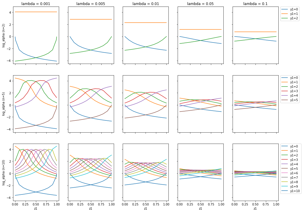 |
| Optimal values of for different values of the hyperparameter |
Loss function
For the loss function for -calibration, we use a variant of in equation (7) as follows:
| (50) |
where denotes the Dirichlet multinomial distribution, and a regularization term is introduced for stabilization purpose, which penalizes the deviation from to both directions towards extreme concentrations of the mass: with or with . We employ throughout this study.
Hyperparameter analysis for the optimal values of
Intuitively, is likely to get close to zero as the regularization coefficient increases. If we regard as a free parameter, the optimal value of only depends on the CPEs , the number of labels and the observed labels for each instance. We assume that the number of labels is common for all the instances for simplicity. The optimality condition for is obtained by taking a derivative of equation (50) with respect to as follows:
| (51) |
where denotes the digamma function, and a recurrence formula is used for the derivation.
One can verify that divergences of the optimal occur in some special cases with . For example, if the labels are unanimous, i.e., , , and , the r.h.s. of equation (51) turns out to be positive as follows:
which implies that . In contrast, if , , and , the r.h.s of equation (51) is calculated as follows:
which results in .
For a finite , the optimal values of can be numerically evaluated by Newton’s method. We show these values in Fig. 3 for several conditions of binary class problems. As expected, the range of the optimal contains zero and gets narrower as increases.
D.3 Proof for Theorem 1
Restatement of Theorem 1.
There exist intervals for parameter , which improve task performances as follows.
- 1.
For DPEs, holds when , and takes the minimum value when , if is satisfied.
- 2.
For posterior CPEs, holds when , and takes the minimum value when , if is satisfied.
Note that we denote , , , and . The optimal of both tasks coincide to be , if CPEs match the true conditional class probabilities given , i.e., .
Proof.
We will omit the superscript from and for brevity. First, we rewrite and in equation (19) as follows:
| (52) |
where . Note that since . We also introduce the following variables:
| (53) | ||||||||
| (54) | ||||||||
| (55) | ||||||||
where, all the variables reside within since .
1. The first statement: DPE
The objective function to be minimized is as follows:
| (56) | ||||
| (57) |
where we use the relation and . Note that only the first term is varied with , and . The condition for satisfying is found by solving
| (58) |
and are trivial solutions that correspond to a hard label prediction (i.e., ) and , respectively. The remaining condition for is
| (59) |
which is feasible when , i.e., . In this case,
| (60) |
is the optimal solution for . By using a relation with equations (59) and (60), the first statement of the theorem is obtained as follows:
| (61) |
If is satisfied, holds, and the above conditions become as follows:
| (62) |
2. The second statement: posterior CPE
The objective for the second problem is as follows:
| (63) |
where the first term equals to , and the second and third term are further transformed as follows:
| (64) | ||||
| (65) |
Hence equation (63) can be written as
| (66) |
The condition for satisfying is obtained by solving
| (67) |
If , which means given , is optimal as expected. For the other case, i.e., , that satisfying and the optimal are
| (68) |
respectively. By using , the corresponding and are
| (69) |
respectively, which are the second statement of the theorem. If is satisfied, holds, and the above conditions become as follows:
| (70) |
Notably, these are the same conditions as the terms in equation (62), respectively. ∎
D.4 Summary of DPE computations
We use -calibration, ensemble-based methods (MCDO and TTA), and a combination of them for predicting DPEs as follows.
-calibration
| (71) |
Ensemble-based methods
| (72) |
where, is the -th prediction of the ensemble, and is the size of the ensemble.
Ensemble-based methods with -calibration
Although an output already represents a CPE distribution without ensemble-based methods: MCDO and TTA, it can be formally combined with these methods. In such cases, we calculate the predictive probability as follows:
| (73) |
where denote the -th ensembles of and , respectively.
D.5 Summary of posterior CPE computations
We consider a task for updating CPE of instance after an expert annotation . For this task, the posterior CPE distribution is computed from an original (prior) CPE distribution model as follows:
| (74) |
where
| (75) |
For the case with multiple test instances, we assume that a predictive model is factorized as follows:
| (76) |
In this case, the posterior of CPEs is also factorized as follows:
| (77) |
-calibration
Prior and posterior CPE distributions are computed as follows:
| (78) | ||||
| (79) |
Ensemble-based methods
Prior and posterior CPE distributions are computed as follows:
| (80) | ||||
| (81) |
where is the size of the ensemble, denotes the -th CPEs of the ensemble, , and .
We omit the cases of predictive models combining the ensemble-based methods and -calibration, where the posterior computation requires further approximation.
D.6 Discussion on conditional i.i.d. assumption of label generations for -calibration
At the beginning of section 3, we assume a conditional i.i.d distribution for labels given input data , which is also a basis for -calibration. We expect that the assumption roughly holds in typical scenarios, where experts are randomly assigned to each example. However, -calibration may not be suitable for counter-examples that break the assumption. For instance, if two fixed experts with different policy annotate all examples, these two labels would be highly correlated. In such a case, the disagreement probability between them may be up to one and exceeds the maximum possible value allowed in equation (19), where always decreases from the original value, which corresponds to , by -calibration.
Appendix E Experimental details
We used the Keras Framework with Tensorflow backend Chollet et al. 2015 for implementation.
E.1 Preprocessing
Mix-MNIST and CIFAR-10
We generated two synthetic image dataset: Mix-MNIST and Mix-CIFAR-10 from MNIST LeCun et al. 2010 and CIFAR-10 Krizhevsky et al. 2009, respectively. We randomly selected half of the images to create mixed-up images from pairs and the other half were retained as original. For each of the paired images, a random ratio that followed a uniform distribution was used for the mix-up and a class probability of multiple labels, which were two or five in validation set. For Mix-MNIST (Mix-CIFAR-10), the numbers of generated instances were , , and for training, validation, and test set, respectively.
MDS Data
We used blood cell images with a size of , which was a part of the dataset obtained in a study of myelodysplastic syndrome (MDS) Sasada et al. 2018, where most of the images showed a white blood cell in the center of the image. For each image, a mean of medical technologists annotated the cellular category from subtypes, in which six were anomalous types. We partitioned the dataset into training, validation, and test set with , , and images, respectively, where each of the partition consisted of images from distinct patient groups. Considering the high labeling cost with experts in the medical domain, we focused on scenarios that training instances were singly labeled, and multiple labels were only available for validation and test set. The mean number of labels per instance for validation and test set were and , respectively.
E.2 Deep neural network architecture
Mix-MNIST
For Mix-MNIST dataset, we used a neural network architecture with three convolutional and two full connection layers. Specifically, the network had the following stack:
- •
Conv. layer with channels, kernel, and ReLU activation
- •
Max pooling with with kernel and same padding
- •
Conv. layer with channels, kernel, and ReLU activation
- •
Max pooling with with kernel and same padding
- •
Conv. layer with channels, kernel, and ReLU activation
- •
Global average pooling with dim. output
- •
Dropout with rate
- •
Full connection layer with dim. output and softmax activation
Mix-CIFAR-10 and MDS
We adopted a modified VGG16 architecture Simonyan and Zisserman 2014 as a base model, in which the full connection layers were removed, and the last layer was a max-pooling with output dimensions. On top of the base model, we appended the following layers:
- •
Dropout with rate and dim. output
- •
Full connection layer with dim. output and ReLU activation
- •
Dropout with rate and dim. output
- •
Full connection layer with dim. output and softmax activation
E.3 Training
We used the following loss function for training:
| (82) |
which was equivalent to the negative log-likelihood for instance-wise multinomial observational model except for constant. We used Adam optimizer Kingma and Ba 2014 with a base learning rate of . Below, we summarize conditions specfic to each dataset.
Mix-MNIST
We trained for a maximum of epochs with a minibatch size of , applying early stopping with ten epochs patience for the validation loss improvement. We used no data augmentation for Mix-MNIST.
Mix-CIFAR-10
We trained for a maximum of epochs with a minibatch size of , applying a variant of warm-up and multi-step decay scheduling He et al. 2016 as follows:
- •
A warm-up with five epochs
- •
A multi-step decay that multiplies the learning rate by at the end of and epochs
We selected the best weights in terms of validation loss. While training, we applied data augmentation with random combinations of the following transformations:
- •
Rotation within to degrees
- •
Width and height shift within pixels
- •
Horizontal flip
MDS
We trained for a maximum of epochs with a minibatch size of , applying a warm-up and multi-step decay scheduling as follows:
- •
A warm-up with five epochs
- •
A multi-step decay that multiplies the learning rate by at the end of , , and epochs
We recorded training weights for every five epochs, and selected the best weights in terms of validation loss. While training, we applied data augmentation with random combinations of the following transformations:
- •
Rotation within to degrees
- •
Width and height shift within pixels
- •
Horizontal flip
For each image, the center portion is cropped from the image after the data augmentation.
E.4 Post-hoc calibrations and predictions
We applied temperature scaling for CPE calibration and -calibration for obtaining CPE distributions. For both calibration methods, we used validation set, which was splited into calibration set for training and calibration-validation (cv) set for the validation of calibration. We trained for a maximum of epochs using Adam optimizer with a learning rate of , applying early stopping with ten epochs patience for the cv loss improvement. The loss functions of equation (82) and (50) were used for CPE- and -calibration, respectively. For the feature layer that used for -calibration, we chose the penultimate layer that corresponded to the last dropout layer in this experiment. The training scheme is the same as that of the CPE calibration, except for a loss function that we described in 3. We also used ensemble-based methods: Monte-Calro dropout (MCDO) Gal and Ghahramani 2016 and Test-time augmentation (TTA) Ayhan and Berens 2018 for CPE distribution predictions, which were both applicable to DNNs at prediction-time, where MC-samples were used for ensemble. A data augmentation applied in TTA was the same as that used in training, and we only applied TTA for Mix-CIFAR-10 and MDS data.
Appendix F Additional experiments
F.1 Evaluations of class probability estimates
We present evaluation results of class probability estimates (CPEs) for Mix-MNIST and Mix-CIFAR-10 in Table 4 and 5, respectively. Overall, CPE measures were comparable between the same datasets with different validation labels (two and five). By comparing and , the relative ratio of against irreducible loss could be evaluated which was much higher in Mix-CIFAR-10 than in Mix-MNIST. Among Raw predictions, temperature scaling kept accuracy and showed a consistent improvement in and as expected. While TTA showed a superior performance over MCDO and Raw predictions in accuracy, and , the effect of calibration methods for CPEs with ensemble-based predictions was not consistent, which might be because calibration was not ensemble-aware.
| Mix-MNIST(2) | Mix-MNIST(5) | |||||||
|---|---|---|---|---|---|---|---|---|
| Method | Acc | Acc | ||||||
| Raw | .9629 | .1386 | .0388 | .0518 | .9629 | .1386 | .0388 | .0518 |
| Raw+ | .9629 | .1386 | .0388 | .0518 | .9629 | .1386 | .0388 | .0518 |
| Raw+ts | .9629 | .1376 | .0379 | .0473 | .9629 | .1376 | .0379 | .0475 |
| Raw+ts+ | .9629 | .1376 | .0379 | .0473 | .9629 | .1376 | .0379 | .0475 |
| MCDO | .9635 | .1392 | .0395 | .0425 | .9635 | .1392 | .0395 | .0425 |
| MCDO+ | .9621 | .1391 | .0394 | .0442 | .9644 | .1387 | .0389 | .0463 |
| MCDO+ts | .9628 | .1408 | .0410 | .0632 | .9627 | .1402 | .0404 | .0638 |
| MCDO+ts+ | .9624 | .1412 | .0415 | .0653 | .9629 | .1407 | .0409 | .0631 |
| Mix-CIFAR-10(2) | Mix-CIFAR-10(5) | |||||||
|---|---|---|---|---|---|---|---|---|
| Method | Acc | Acc | ||||||
| Raw | .7965 | .3518 | .2504 | .1093 | .7965 | .3518 | .2504 | .1093 |
| Raw+ | .7965 | .3518 | .2504 | .1093 | .7965 | .3518 | .2504 | .1093 |
| Raw+ts | .7965 | .3437 | .2423 | .0687 | .7965 | .3438 | .2423 | .0685 |
| Raw+ts+ | .7965 | .3437 | .2423 | .0688 | .7965 | .3438 | .2423 | .0685 |
| MCDO | .7983 | .3488 | .2474 | .0955 | .7983 | .3488 | .2474 | .0955 |
| MCDO+ | .7968 | .3488 | .2474 | .0962 | .7965 | .3493 | .2479 | .0973 |
| MCDO+ts | .7972 | .3442 | .2428 | .0684 | .7977 | .3446 | .2431 | .0675 |
| MCDO+ts+ | .7965 | .3445 | .2430 | .0650 | .7975 | .3444 | .2430 | .0723 |
| TTA | .8221 | .3230 | .2216 | .0877 | .8221 | .3230 | .2216 | .0877 |
| TTA+ | .8241 | .3221 | .2206 | .0884 | .8277 | .3223 | .2209 | .0894 |
| TTA+ts | .8257 | .3467 | .2452 | .1688 | .8279 | .3466 | .2451 | .1707 |
| TTA+ts+ | .8277 | .3446 | .2432 | .1697 | .8245 | .3460 | .2446 | .1726 |
F.2 Discussion on the effect of temperature scaling for disagreement probability estimates
 |
| Changes in the maximum CPEs and DPEs with temperature scaling |
In Table 1, it is observed that disagreement probability estimates (DPEs) are consistently degraded by temperature scaling (Raw+ts) from the original scores (Raw), despite the positive effects for calibration of class probability estimates (CPEs) with ts. Though we observe that the degradation can be overcome with -calibration (see Raw+ts+ or Raw+ in Table 1), the mechanism that causes the phenomena is worth analyzing. Since there exists well-known overconfidence in the maximum class probabilities from DNN classifiers Guo et al. 2017, the recalibration of CPEs by ts tends to reduce the maximum class probabilities. On the other hand, the amount of change in a DPE for each instance can be written as follows:
| (83) |
where and denote the original CPEs and DPE, respectively, and and denote those after ts, respectively. It is likely that takes a positive value as the dominant term of in equation (83) is with the maximum value, where is satisfied for overconfident predictions. In fact, the averages of between Raw+ts and Raw for each of the five settings in Table 1 are all positive, which are , , , , and , respectively. Instance-wise changes in the maximum CPEs and DPEs with ts are shown in Fig. 4. Simultaneously, DPEs without -calibration systematically overestimate the empirical disagreement probabilities, as shown in Fig. 1. Therefore, the positive means that is even far from a target probability than is, despite the improvement in CPEs with ts.
F.3 Additional experiments for MDS data
In addition to MDS data with single training labels per instance (MDS-1) used in the main experiment, we trained and evaluated with full MDS data (MDS-full), where all the multiple training labels per example were employed. Also, we included additional CPE calibration methods: vector and matrix scaling (vs and ms, respectively), which were introduced in Section D.1, for these experiments. We adopted an L2 regularization for vs and an ODIR for ms, in which the following hyper-parameter candidates were examined:
- •
vs:
- •
ms:
where and were defined in equation (48) and (49), respectively. The hyper-parameters were selected with respect to the best cv loss, which were for vs and for ms in the single-training MDS data, and for vs and for ms in the full MDS data.
Results
We summarize the order-1 and -2 performance metrics for predictions with MDS-1 and MDS-full datasets in Table 6. For both datasets, temperature scaling consistently improved (decreased) and for each of Raw, MCDO, and TTA predictions. While vector scaling was slightly better at obtaining the highest accuracy than the other methods, the effect of vs and ms for the metrics of probability predictions were limited. As same as the results of synthetic experiments, TTA showed a superior performance over MCDO and Raw predictions in accuracy, and . Since can be decomposed into and the remaining term: (Section B.4), the difference of predictors in CPE performance is clearly presented with 2d plots (Fig.5 and 6), which we call calibration-dispersion maps. For order-2 metrics, both and for DPEs were substantially improved by -calibration, espetially in , which was not attained with solely applying ensemble-based methods even with MDS-full. This improvement of DPE calibration was also visually confirmed with reliability diagrams in Fig. 5 and 6. Though overall characteristics were similar between MDS-1 and MDS-full, a substantial improvement in , , and was observed in MDS-full, which seemed the results of enhanced probability predictions with additional training labels.
| MDS-1 | MDS-full | |||||||||||
|---|---|---|---|---|---|---|---|---|---|---|---|---|
| Order-1 metrics | Order-2 metrics | Order-1 metrics | Order-2 metrics | |||||||||
| Method | Acc | Acc | ||||||||||
| Raw | .9006 | .2515 | .0435 | .0600 | .1477 | .0628 | .8990 | .2460 | .0380 | .0590 | .1448 | .0539 |
| Raw+ | .9006 | .2515 | .0435 | .0600 | .1454 | .0406 | .8990 | .2460 | .0380 | .0590 | .1430 | .0320 |
| 05mm. Raw+ts | .9006 | .2509 | .0430 | .0575 | .1482 | .0663 | .8990 | .2459 | .0379 | .0587 | .1449 | .0545 |
| Raw+ts+ | .9006 | .2509 | .0430 | .0575 | .1445 | .0261 | .8990 | .2459 | .0379 | .0587 | .1427 | .0269 |
| 05mm. Raw+vs | .9010 | .2515 | .0435 | .0579 | .1489 | .0696 | .8996 | .2461 | .0381 | .0602 | .1452 | .0563 |
| Raw+vs+ | .9010 | .2515 | .0435 | .0579 | .1449 | .0318 | .8996 | .2461 | .0381 | .0602 | .1431 | .0310 |
| 05mm. Raw+ms | .8992 | .2532 | .0453 | .0656 | .1484 | .0663 | .8978 | .2480 | .0400 | .0710 | .1451 | .0563 |
| Raw+ms+ | .8992 | .2532 | .0453 | .0656 | .1453 | .0355 | .8978 | .2480 | .0400 | .0710 | .1428 | .0274 |
| MCDO | .8983 | .2517 | .0437 | .0586 | .1470 | .0562 | .8989 | .2460 | .0380 | .0561 | .1446 | .0505 |
| MCDO+ | .8996 | .2518 | .0438 | .0610 | .1450 | .0346 | .9003 | .2458 | .0378 | .0568 | .1426 | .0237 |
| 05mm. MCDO+ts | .8986 | .2515 | .0435 | .0579 | .1479 | .0635 | .8995 | .2458 | .0378 | .0579 | .1447 | .0521 |
| MCDO+ts+ | .8991 | .2515 | .0435 | .0586 | .1442 | .0186 | .8997 | .2460 | .0380 | .0581 | .1423 | .0180 |
| 05mm. MCDO+vs | .8997 | .2521 | .0441 | .0589 | .1487 | .0664 | .9004 | .2461 | .0381 | .0593 | .1448 | .0531 |
| MCDO+vs+ | .9009 | .2519 | .0439 | .0575 | .1446 | .0244 | .9002 | .2460 | .0380 | .0579 | .1426 | .0228 |
| 05mm. MCDO+ms | .8970 | .2536 | .0456 | .0678 | .1479 | .0612 | .8997 | .2477 | .0397 | .0704 | .1448 | .0529 |
| MCDO+ms+ | .8986 | .2534 | .0454 | .0667 | .1449 | .0279 | .8986 | .2478 | .0399 | .0695 | .1424 | .0188 |
| TTA | .9013 | .2458 | .0378 | .0642 | .1441 | .0488 | .9069 | .2402 | .0322 | .0645 | .1425 | .0444 |
| TTA+ | .9025 | .2456 | .0376 | .0684 | .1428 | .0334 | .9077 | .2402 | .0322 | .0650 | .1413 | .0277 |
| 05mm. TTA+ts | .9012 | .2459 | .0379 | .0646 | .1448 | .0553 | .9074 | .2401 | .0321 | .0636 | .1425 | .0456 |
| TTA+ts+ | .9011 | .2458 | .0378 | .0632 | .1422 | .0197 | .9055 | .2403 | .0323 | .0633 | .1410 | .0204 |
| 05mm. TTA+vs | .9031 | .2471 | .0392 | .0671 | .1458 | .0598 | .9078 | .2409 | .0329 | .0666 | .1431 | .0483 |
| TTA+vs+ | .9025 | .2470 | .0391 | .0657 | .1428 | .0247 | .9068 | .2409 | .0329 | .0664 | .1416 | .0252 |
| 05mm. TTA+ms | .9001 | .2489 | .0410 | .0756 | .1456 | .0561 | .9034 | .2429 | .0349 | .0778 | .1431 | .0481 |
| TTA+ms+ | .8991 | .2487 | .0407 | .0750 | .1431 | .0268 | .9030 | .2432 | .0352 | .0766 | .1414 | .0213 |
 |
|
| (a) Calibration-dispersion map | (b) Reliability diagram for disagreement probability |
 |
 |
| (a) Calibration-dispersion map | (b) Reliability diagram for disagreement probability |