NeuMiss networks: differentiable programming for supervised learning with missing values
Abstract
The presence of missing values makes supervised learning much more challenging. Indeed, previous work has shown that even when the response is a linear function of the complete data, the optimal predictor is a complex function of the observed entries and the missingness indicator. As a result, the computational or sample complexities of consistent approaches depend on the number of missing patterns, which can be exponential in the number of dimensions. In this work, we derive the analytical form of the optimal predictor under a linearity assumption and various missing data mechanisms including Missing at Random (MAR) and self-masking (Missing Not At Random). Based on a Neumann-series approximation of the optimal predictor, we propose a new principled architecture, named NeuMiss networks. Their originality and strength come from the use of a new type of non-linearity: the multiplication by the missingness indicator. We provide an upper bound on the Bayes risk of NeuMiss networks, and show that they have good predictive accuracy with both a number of parameters and a computational complexity independent of the number of missing data patterns. As a result they scale well to problems with many features, and remain statistically efficient for medium-sized samples. Moreover, we show that, contrary to procedures using EM or imputation, they are robust to the missing data mechanism, including difficult MNAR settings such as self-masking.
1 Introduction
Increasingly complex data-collection pipelines, often assembling multiple sources of information, lead to datasets with incomplete observations and complex missing-values mechanisms. The pervasiveness of missing values has triggered an abundant statistical literature on the subject [14, 31]: a recent survey reviewed more than 150 implementations to handle missing data [10]. Nevertheless, most methods have been developed either for inferential purposes, i.e. to estimate parameters of a probabilistic model of the fully-observed data, or for imputation, completing missing entries as well as possible [6]. These methods often require strong assumptions on the missing-values mechanism, i.e. either the missing at random (MAR) assumption [27] – the probability of being missing only depends on observed values – or the more restrictive Missing Completely At Random assumption (MCAR) – the missingness is independent of the data. In MAR or MCAR settings, good imputation is sufficient to fit statistical models, or even train supervised-learning models [11]. In particular, a precise knowledge of the data-generating mechanism can be used to derive an Expectation Maximization (EM) [2] formulation with the minimum number of necessary parameters. Yet, as we will see, this is intractable if the number of features is not small, as potentially missing-value patterns must be modeled.
The last missing-value mechanism category, Missing Not At Random (MNAR), covers cases where the probability of being missing depends on the unobserved values. This is a frequent situation in which missingness cannot be ignored in the statistical analysis [12]. Much of the work on MNAR data focuses on problems of identifiability, in both parametric and non-parametric settings [29, 20, 21, 22]. In MNAR settings, estimation strategies often require modeling the missing-values mechanism [9]. This complicates the inference task and is often limited to cases with few MNAR variables. Other approaches need the masking matrix to be well approximated with low-rank matrices [18, 1, 7, 16, 32].
Supervised learning with missing values has different goals than probabilistic modeling [11] and has been less studied. As the test set is also expected to have missing entries, optimality on the fully-observed data is no longer a goal per se. Rather, the goal of minimizing an expected risk lend itself well to non-parametric models which can compensate from some oddities introduced by missing values. Indeed, with a powerful learner capable of learning any function, imputation by a constant is Bayes consistent [11]. Yet, the complexity of this function that must be approximated governs the success of this approach outside of asymptotic regimes. In the simple case of a linear regression with missing values, the optimal predictor has a combinatorial expression: for features, there are possible missing-values patterns requiring models [13].
Le Morvan et al. 2020 showed that in this setting, a multilayer perceptrons (MLP) can be consistent even in a pattern mixture MNAR model, but assuming hidden units. There have been many adaptations of neural networks to missing values, often involving an imputation with 0’s and concatenating the mask (the indicator matrix coding for missing values) [23, 19, 15, 34, 4]. However there is no theory relating the network architecture to the impact of the missing-value mechanism on the prediction function. In particular, an important practical question is: how complex should the architecture be to cater for a given mechanism? Overly-complex architectures require a lot of data, but being too restrictive will introduce bias for missing values.
The present paper addresses the challenge of supervised learning with missing values. We propose a theoretically-grounded neural-network architecture which allows to implicitly impute values as a function of the observed data, aiming at the best prediction. More precisely,
- •
We derive an analytical expression of the Bayes predictor for linear regression in the presence of missing values under various missing data mechanisms including MAR and self-masking MNAR.
- •
We propose a new principled architecture, named NeuMiss network, based on a Neumann series approximation of the Bayes predictors, whose originality and strength is the use of nonlinearities, i.e. the elementwise multiplication by the missingness indicator.
- •
We provide an upper bound on the Bayes risk of NeuMiss networks which highlights the benefits of depth and learning to approximate.
- •
We provide an interpretation of a classical ReLU network as a shallow NeuMiss network. We further demonstrate empirically the crucial role of the nonlinearities, by showing that increasing the capacity of NeuMiss networks improves predictions while it does not for classical networks.
- •
We show that NeuMiss networks are suited medium-sized datasets: they require samples, contrary to for methods that do not share weights between missing data patterns.
- •
We demonstrate the benefits of the proposed architecture over classical methods such as EM algorithms or iterative conditional imputation [31] both in terms of computational complexity –these methods scale in [28] and respectively–, and in the ability to be robust to the missing data mechanism, including MNAR.
2 Optimal predictors in the presence of missing values
Notations
We consider a data set of independent pairs , distributed as the generic pair , where and . We introduce the indicator vector which satisfies, for all , if and only if is not observed. The random vector acts as a mask on . We define the incomplete feature vector (see [27], [26, appendix B]) as if , and otherwise. As such, is a mixed categorical and continuous variable. An example of realization (lower-case letters) of the previous random variables would be a vector with the missing pattern , giving
For realizations of , we also denote by (resp. ) the indices of the zero entries of (resp. non-zero). Following classic missing-value notations, we let (resp. ) be the observed (resp. missing) entries in . Pursuing the above example, we have , , , . To lighten notations, when there is no ambiguity, we remove the explicit dependence in and write, e.g., .
2.1 Problem statement: supervised learning with missing values
We consider a linear model of the complete data, such that the response satisfies:
| (1) |
Prediction with missing values departs from standard linear-model settings: the aim is to predict given , as the complete input may be unavailable. The corresponding optimization problem is:
| (2) |
where is the Bayes predictor for the squared loss, in the presence of missing values. The main difficulty of this problem comes from the half-discrete nature of the input space . Indeed, the Bayes predictor can be rewritten as:
| (3) |
which highlights the combinatorial issue of solving (2): one may need to optimize submodels, for the different . In the following, we write the Bayes predictor as a function of :
2.2 Expression of the Bayes predictor under various missing-values mechanisms
There is no general closed-form expression for the Bayes predictor, as it depends on the data distribution and missingness mechanism. However, an exact expression can be derived for Gaussian data with various missingness mechanisms.
Assumption 1 (Gaussian data).
The distribution of is Gaussian, that is, .
Assumption 2 (MCAR mechanism).
For all , .
Assumption 3 (MAR mechanism).
For all , .
Proposition 2.1 (MAR Bayes predictor).
Obtaining the Bayes predictor expression turns out to be far more complicated for general MNAR settings but feasible for the Gaussian self-masking mechanism described below.
Assumption 4 (Gaussian self-masking).
The missing data mechanism is self-masked with and
Proposition 2.2 (Bayes predictor with Gaussian self-masking).
The proof of Propositions 2.1 and 2.2 are in the Supplementary Materials (A.3 and A.4). These are the first results establishing exact expressions of the Bayes predictor in a MAR and specific MNAR mechanisms. Note that these propositions show that the Bayes predictor is linear by pattern under the assumptions studied, i.e., each of the submodels in equation 3 are linear functions of . For non-Gaussian data, the Bayes predictor may not be linear by pattern [13, Example 3.1].
Generality of the Gaussian self-masking model
For a self-masking mechanism where the probability of being missing increases (or decreases) with the value of the underlying variable, probit or logistic functions are often used [12]. A Gaussian self-masking model is also a suitable model: setting the mean of the Gaussian close to the extreme values gives a similar behaviour. In addition, it covers cases where the probability of being missing is centered around a given value.
3 NeuMiss networks: learning by approximating the Bayes predictors
3.1 Insight to build a network: sharing parameters across missing-value patterns
Computing the Bayes predictors in equations (4) or (2.2) requires to estimate the inverse of each submatrix for each missing-data pattern , ie one linear model per missing-data pattern. For a number of hidden units , a MLP with ReLU non-linearities can fit these linear models independently from one-another, and is shown to be consistent [13]. But it is prohibitive when grows. Such an architecture is largely over-parametrized as it does not share information between similar missing-data patterns. Indeed, the slopes of each of the linear regression per pattern given by the Bayes predictor in equations (4) and (2.2) are linked via the inverses of .
Thus, one approach is to estimate only one vector and one covariance matrix via an expectation maximization (EM) algorithm [2], and then compute the inverses of . But the computational complexity then scales linearly in the number of missing-data patterns (which is in the worst case exponential in the dimension ), and is therefore also prohibitive when the dimension increases.
In what follows, we propose an in-between solution, modeling the relationships between the slopes for different missing-data patterns without directly estimating the covariance matrix. Intuitively, observations from one pattern will be used to estimate the regression parameters of other patterns.
3.2 Differentiable approximations of the inverse covariances with Neumann series
The major challenge of equations (4) and (2.2) is the inversion of the matrices for all . Indeed, there is no simple relationship for the inverses of different submatrices in general. As a result, the slope corresponding to a pattern cannot be easily expressed as a function of .
We therefore propose to approximate for all recursively in the following way. First, we choose as a starting point a matrix . is then defined as the sub-matrix of obtained by selecting the columns and rows that are observed (components for which ) and is our order- approximation of . Then, for all , we define the order- approximation of via the following iterative formula: for all ,
| (6) |
The iterates converge linearly to (A.5 in the Supplementary Materials), and are in fact Neumann series truncated to terms if .
We now define the order- approximation of the Bayes predictor in MAR settings (equation (4)) as
| (7) |
The error between the Bayes predictor and its order- approximation is provided in Proposition 3.1.
Proposition 3.1.
The error of the order- approximation decays exponentially fast with . More importantly, if the submatrices of are good approximations of on average, that is if we choose which minimizes the expectation in the right-hand side in inequality (8), then our model provides a good approximation of the Bayes predictor even with order . This is the case for a diagonal covariance matrix, as taking has no approximation error as .
3.3 NeuMiss network architecture: multiplying by the mask
Network architecture
We propose a neural-network architecture to approximate the Bayes predictor, where the inverses are computed using an unrolled version of the iterative algorithm. Figure 1 gives a diagram for such neural network using an order-3 approximation corresponding to a depth 4. is the input, with missing values replaced by 0. is a trainable parameter corresponding to the parameter in equation (7). To match the Bayes predictor exactly (equation (7)), weight matrices should be simple transformations of the covariance matrix indicated in blue on Figure 1.
Following strictly Neummann iterates would call for a shared weight matrix across all . Rather, we learn each layer independently. This choice is motivated by works on iterative algorithm unrolling [5] where independent layers’ weights can improve a network’s approximation performance [33]. Note that [3] has also introduced a neural network architecture based on unrolling the Neumann series. However, their goal is to solve a linear inverse problem with a learned regularization, which is very different from ours.
Multiplying by the mask
Note that the observed indices change for each sample, leading to an implementation challenge. For a sample with missing data pattern , the weight matrices , and of Figure 1 should be masked such that their rows and columns corresponding to the indices are zeroed, and the rows of corresponding to as well as the columns of corresponding to are zeroed. Implementing efficiently a network in which the weight matrices are masked differently for each sample can be challenging. We thus use the following trick. Let be a weight matrix, a vector, and . Then , i.e, using a masked weight matrix is equivalent to masking the input and output vector. The network can then be seen as a classical network where the nonlinearities are multiplications by the mask.
Approximation of the Gaussian self-masking Bayes predictor
Although our architecture is motivated by the expression of the Bayes predictor in MCAR and MAR settings, a similar architecture can be used to target the prediction function (2.2) for self-masking data. To see why, let’s first assume that . Then, the self-masking Bayes predictor (2.2) becomes:
| (9) |
i.e., its expression is the same as for the M(C)AR Bayes predictor (4) except that is replaced by and is scaled down by a factor . Thus, under this approximation, the self-masking Bayes predictor can be modeled by our proposed architecture (just as the M(C)AR Bayes predictor), the only difference being the targeted values for the parameters and of the network. A less coarse approximation also works: where is a diagonal matrix. In this case, the proposed architecture can perfectly model the self-masking Bayes predictor: the parameter of the network should target and should target instead of simply in the M(C)AR case. Consequently, our architecture can well approximate the self-masking Bayes predictor by adjusting the values learned for the parameters and if are close to diagonal matrices.
3.4 Link with the multilayer perceptron with ReLU activations
A common practice to handle missing values is to consider as input the data concatenated with the mask eg in [13]. The next proposition connects this practice to Neumman networks.
Proposition 3.2 (equivalence MLP - depth-1 NeuMiss network).
Let be an input imputed by 0 concatenated with the mask .
- •
Let be a hidden layer which connects to hidden units, and applies a ReLU nonlinearity to the activations.
- •
Let be a hidden layer that connects an input to hidden units, and applies a nonlinearity.
Denote by and the outputs of the hidden unit of each layer. Then there exists a configuration of the weights of the hidden layer such that and have the same hidden units activated for any , and activated hidden units are such that where .
Proposition 3.2 states that a hidden layer can be rewritten as a layer up to a constant. Note that, as soon as another layer is stacked after or , this additional constant can be absorbed into the biases of this new layer. Thus the weights of can be learned so as to mimic . In our case, this means that a MLP with ReLU activations, one hidden layer of hidden units, and which operates on the concatenated vector, is closely related to the -depth NeuMiss network (see Figure 1), thereby providing theoretical support for the use of the latter MLP. This theoretical link completes the results of [13], who showed experimentally that in such a MLP units were enough to perform well on Gaussian data, but only provided theoretical results with hidden units.
4 Empirical results
4.1 The nonlinearity is crucial to the performance
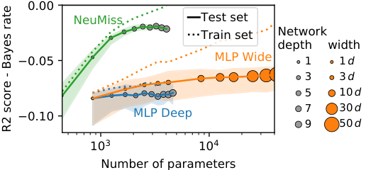
The specificity of NeuMiss networks resides in the nonlinearities, instead of more conventional choices such as ReLU. Figure 2 shows how the choice of nonlinearity impacts the performance as a function of the depth. We compare two networks that take as input the data imputed by 0 concatenated with the mask: MLP Deep which has 1 to 10 hidden layers of hidden units followed by ReLU nonlinearities and MLP Wide which has one hidden layer whose width is increased followed by a ReLU nonlinearity. This latter was shown to be consistent given hidden units [13].
Figure 2 shows that increasing the capacity (depth) of MLP Deep fails to improve the performances, unlike with NeuMiss networks. Similarly, it is also significantly more effective to increase the capacity of the NeuMiss network (depth) than to increase the capacity (width) of MLP Wide. These results highlight the crucial role played by the nonlinearity. Finally, the performance of MLP Wide with hidden units is close to that of NeuMiss with a depth of 1, suggesting that it may rely on the weight configuration established in Proposition 3.2.
4.2 Approximation learned by the NeuMiss network
The NeuMiss architecture was designed to approximate well the Bayes predictor (4). As shown in Figure 1, its weights can be chosen so as to express the Neumann approximation of the Bayes predictor (7) exactly. We will call this particular instance of the network, with set to identity, the analytic network. However, just like LISTA [5] learns improved weights compared to the ISTA iterations, the NeuMiss network may learn improved weights compared to the Neumann iterations. Comparing the performance of the analytic network to its learned counterpart on simulated MCAR data, Figure 3 (left) shows that the learned network requires a much smaller depth compared to the analytic network to reach a given performance. Moreover, the depth-1 learned network largely outperforms the depth-1 analytic network, which means that it is able to learn a good initialization for the iterates. Figure 3 also compares the performance of the learned network with and without residual connections, and shows that residual connections are not needed for good performance. This observation is another hint that the iterates learned by the network depart from the Neumann ones.
4.3 NeuMiss networks require samples
Figure 3 (right) studies the depth for which NeuMiss networks perform well for different number of samples and features . It outlines that NeuMiss networks work well in regimes with more than 10 samples available per model parameters, where the number of model parameters scales as . In general, even with many samples, depth of more than 5 explore diminishing returns. Supplementary figure 5 shows the same behavior in various MNAR settings.
MCAR
4.4 Prediction performance: NeuMiss networks are robust to the missing data mechanism
We now evaluate the performance of NeuMiss networks compared to other methods under various missing values mechanisms. The data are generated according to a multivariate Gaussian distribution, with a covariance matrix , , and the entries of drawn from a standard normal distribution. The noise is a vector of entries drawn uniformly in to make full rank. The mean is drawn from a standard normal distribution. The response is generated as a linear function of the complete data as in equation 1. The noise is chosen to obtain a signal-to-noise ratio of 10. 50% of entries on each features are missing, with various missing data mechanisms: MCAR, MAR, Gaussian self-masking and Probit self-masking. The Gaussian self-masking is obtained according to Assumption 4, while the Probit self-masking is a similar setting where the probability for feature to be missing depends on its value through an inverse probit function. We compare the performances of the following methods:
- •
EM: an Expectation-Maximisation algorithm [30] is run to estimate the parameters of the joint probability distribution of and –Gaussian– with missing values. Then based on this estimated distribution, the prediction is given by taking the expectation of given .
- •
- •
MLP: A multilayer perceptron as in [13], with one hidden layer followed by a ReLU nonlinearity, taking as input the data imputed by 0 concatenated with the mask. The width of the hidden layer is varied between and hidden units, and chosen using a validation set. The MLP is trained using ADAM and a batch size of 200. The learning rate is initialized to and decreased by a factor of 0.2 when the loss stops decreasing for 2 epochs. The training finishes when either the learning rate goes below or the maximum number of epochs is reached.
- •
NeuMiss : The NeuMiss architecture, without residual connections, choosing the depth on a validation set. The architecture was implemented using PyTorch [24], and optimized using stochastic gradient descent and a batch size of 10. The learning rate schedule and stopping criterion are the same as for the MLP.
MCAR Gaussian self-masking Probit self-masking
For MCAR, MAR, and Gaussian self-masking settings, the performance is given as the obtained R2 score minus the Bayes rate (the closer to 0 the better), the best achievable R2 knowing the underlying ground truth parameters. In our experiments, an estimation of the Bayes rate is obtained using the score of the Bayes predictor. For probit self-masking, as we lack an analytical expression for the Bayes predictor, the performance is given with respect to the best performance achieved across all methods. The code to reproduce the experiments is available in GitHub 11 1 https://github.com/marineLM/NeuMiss.
In MCAR settings, figure 4 shows that, as expected, EM gives the best results when tractable. Yet, we could not run it for number of features . NeuMiss is the best performing method behind EM, in all cases except for , where depth of 1 or greater overfit due to the low ratio of number of parameters to number of samples. In such situation, MLP has the same expressive power and performs slightly better. Note that for a high samples-to-parameters ratio (), NeuMiss reaches an almost perfect score, less than 1% below the Bayes rate. The results for the MAR setting are very similar to the MCAR results, and are given in supplementary figure 6.
For the self-masking mechanisms, the NeuMiss network significantly improves upon the competitors, followed by the MLP. This is even true for the probit self-masking case for which we have no theoretical results. The gap between the two architectures widens as the number of samples increases, with the NeuMiss network benefiting from a large amount of data. These results emphasize the robustness of NeuMiss and MLP to the missing data mechanism, including MNAR settings in which EM or conditional imputation do not enable statistical analysis.
5 Discussion and conclusion
Traditionally, statistical models are adapted to missing values using EM or imputation. However, these require strong assumptions on the missing values. Rather, we frame the problem as a risk minimization with a flexible yet tractable function family. We propose the NeuMiss network, a theoretically-grounded architecture that handles missing values using multiplication by the mask as nonlinearities. It targets the Bayes predictor with differentiable approximations of the inverses of the various covariance submatrices, thereby reducing complexity by sharing parameters across missing data patterns. Strong connections between a shallow version of our architecture and the common practice of inputing the mask to an MLP is established.
The NeuMiss architecture has clear practical benefits. It is robust to the missing-values mechanism, often unknown in practice. Moreover its sample and computational complexity are independent of the number of missing-data patterns, which allows to work with datasets of higher dimensionality and limited sample sizes. This work opens many perspectives, in particular using this network as a building block in larger architectures, eg to tackle nonlinear problems.
Broader Impact
In our work, we proposed theoretical foundations to justify the use of a specific neural network architecture in the presence of missing-values.
Neural networks are known for their challenging black-box nature. We believe that such theory leads to a better understanding of the mechanisms at work in neural networks.
Our architecture is tailored for missing data. These are present in many applications, in particular in social or health data. In these fields, it is common for under-represented groups to exhibit a higher percentage of missing values (MNAR mechanism). Dealing with these missing values will definitely improve prediction for these groups, thereby reducing potential bias against these exact same groups.
As any predictive algorithm, our proposal can be misused in a variety of context, including in medical science, for which a proper assessment of the specific characteristics of the algorithm output is required (assessing bias in prediction, prevent false conclusion resulting from misinterpreting outputs). Yet, by improving performance and understanding of a fundamental challenge in many applications settings, our work is not facilitating more unethical aspects of AI than ethical applications. Rather, medical studies that suffer chronically from limited sample sizes are mostly likely to benefit from the reduced sample complexity that these advances provide.
Acknowledgments and Disclosure of Funding
This work was funded by ANR-17-CE23-0018 - DirtyData - Intégration et nettoyage de données pour l’analyse statistique (2017) and the MissingBigData grant from DataIA.
References
- Audibert et al. [2011] Jean-Yves Audibert, Olivier Catoni, and Others. Robust linear least squares regression. The Annals of Statistics, 39(5):2766–2794, 2011.
- Dempster et al. [1977] Arthur P Dempster, Nan M Laird, and Donald B Rubin. Maximum likelihood from incomplete data via the EM algorithm. Journal of the royal statistical society. Series B (methodological), pages 1–38, 1977.
- Gilton et al. [2020] D. Gilton, G. Ongie, and R. Willett. Neumann networks for linear inverse problems in imaging. IEEE Transactions on Computational Imaging, 6:328–343, 2020.
- Gong et al. [2020] Yu Gong, Hossein Hajimirsadeghi, Jiawei He, Megha Nawhal, Thibaut Durand, and Greg Mori. Variational selective autoencoder. In Cheng Zhang, Francisco Ruiz, Thang Bui, Adji Bousso Dieng, and Dawen Liang, editors, Proceedings of The 2nd Symposium on Advances in Approximate Bayesian Inference, volume 118 of Proceedings of Machine Learning Research, pages 1–17. PMLR, 08 Dec 2020.
- Gregor and LeCun [2010] Karol Gregor and Yann LeCun. Learning fast approximations of sparse coding. In Proceedings of the 27th International Conference on International Conference on Machine Learning, pages 399–406, 2010.
- Hastie et al. [2015] Trevor Hastie, Rahul Mazumder, Jason D. Lee, and Reza Zadeh. Matrix completion and low-rank svd via fast alternating least squares. J. Mach. Learn. Res., 16(1):3367–3402, January 2015. ISSN 1532-4435.
- Hernández-Lobato et al. [2014] José Miguel Hernández-Lobato, Neil Houlsby, and Zoubin Ghahramani. Probabilistic matrix factorization with non-random missing data. In International Conference on Machine Learning, pages 1512–1520, 2014.
- Hwang [2004] Suk-Geun Hwang. Cauchy’s Interlace Theorem for Eigenvalues of Hermitian Matrices. The American Mathematical Monthly, 111(2):157, February 2004. ISSN 00029890. doi: 10.2307/4145217.
- Ibrahim et al. [1999] Joseph G Ibrahim, Stuart R Lipsitz, and M-H Chen. Missing covariates in generalized linear models when the missing data mechanism is non-ignorable. Journal of the Royal Statistical Society: Series B (Statistical Methodology), 61(1):173–190, 1999.
- Imke Mayer Julie Josse and Vialaneix [2019] Nicholas Tierney Imke Mayer Julie Josse and Nathalie Vialaneix. R-miss-tastic: a unified platform for missing values methods and workflows, 2019.
- Josse et al. [2019] Julie Josse, Nicolas Prost, Erwan Scornet, and Gaël Varoquaux. On the consistency of supervised learning with missing values. arXiv preprint arXiv:1902.06931, 2019.
- Kim and Ying [2018] J K Kim and Z Ying. Data Missing Not at Random, special issue. Statistica Sinica. Institute of Statistical Science, Academia Sinica, 2018.
- Le Morvan et al. [2020] Marine Le Morvan, Nicolas Prost, Julie Josse, Erwan Scornet, and Gaël Varoquaux. Linear predictor on linearly-generated data with missing values: non consistency and solutions. arXiv preprint arXiv:2002.00658, 2020.
- Little and Rubin [2019] Roderick J A Little and Donald B Rubin. Statistical analysis with missing data. John Wiley & Sons, 2019.
- Ma et al. [2018] Chao Ma, Sebastian Tschiatschek, Konstantina Palla, José Miguel Hernández-Lobato, Sebastian Nowozin, and Cheng Zhang. Eddi: Efficient dynamic discovery of high-value information with partial vae. arXiv preprint arXiv:1809.11142, 2018.
- Ma and Chen [2019] Wei Ma and George H Chen. Missing not at random in matrix completion: The effectiveness of estimating missingness probabilities under a low nuclear norm assumption. In Advances in Neural Information Processing Systems, pages 14871–14880, 2019.
- Majumdar and Majumdar [2019] Rajeshwari Majumdar and Suman Majumdar. On the conditional distribution of a multivariate normal given a transformation–the linear case. Heliyon, 5(2):e01136, 2019.
- Marlin and Zemel [2009] Benjamin M Marlin and Richard S Zemel. Collaborative prediction and ranking with non-random missing data. In Proceedings of the third ACM conference on Recommender systems, pages 5–12. ACM, 2009.
- Mattei and Frellsen [2019] Pierre-Alexandre Mattei and Jes Frellsen. MIWAE: Deep generative modelling and imputation of incomplete data sets. In Kamalika Chaudhuri and Ruslan Salakhutdinov, editors, Proceedings of the 36th International Conference on Machine Learning, volume 97 of Proceedings of Machine Learning Research, pages 4413–4423, Long Beach, California, USA, 09–15 Jun 2019. PMLR.
- Miao et al. [2016] Wang Miao, Peng Ding, and Zhi Geng. Identifiability of normal and normal mixture models with nonignorable missing data. Journal of the American Statistical Association, 111(516):1673–1683, 2016.
- Mohan and Pearl [2019] K Mohan and J Pearl. Graphical Models for Processing Missing Data. Technical Report R-473-L, Department of Computer Science, University of California, Los Angeles, CA, 2019.
- Nabi et al. [2020] Razieh Nabi, Rohit Bhattacharya, and Ilya Shpitser. Full law identification in graphical models of missing data: Completeness results. arXiv preprint arXiv:2004.04872, 2020.
- Nazabal et al. [2018] Alfredo Nazabal, Pablo M Olmos, Zoubin Ghahramani, and Isabel Valera. Handling incomplete heterogeneous data using vaes. arXiv preprint arXiv:1807.03653, 2018.
- Paszke et al. [2019] Adam Paszke, Sam Gross, Francisco Massa, Adam Lerer, James Bradbury, Gregory Chanan, Trevor Killeen, Zeming Lin, Natalia Gimelshein, Luca Antiga, et al. Pytorch: An imperative style, high-performance deep learning library. In Advances in Neural Information Processing Systems, pages 8024–8035, 2019.
- Pedregosa et al. [2011] F Pedregosa, G Varoquaux, A Gramfort, V Michel, B Thirion, O Grisel, M Blondel, P Prettenhofer, R Weiss, V Dubourg, J Vanderplas, A Passos, D Cournapeau, M Brucher, M Perrot, and E Duchesnay. Scikit-learn: Machine Learning in Python . Journal of Machine Learning Research, 12:2825–2830, 2011.
- Rosenbaum and Rubin [1984] Paul R Rosenbaum and Donald B Rubin. Reducing bias in observational studies using subclassification on the propensity score. Journal of the American Statistical Association, 79(387):516–524, 1984. doi: 10.2307/2288398.
- Rubin [1976] Donald B Rubin. Inference and missing data. Biometrika, 63(3):581–592, 1976.
- Seber and Lee [2003] George AF Seber and Alan J Lee. Wiley series in probability and statistics. Linear Regression Analysis, pages 36–44, 2003.
- Tang et al. [2003] Gong Tang, Roderick JA Little, and Trivellore E Raghunathan. Analysis of multivariate missing data with nonignorable nonresponse. Biometrika, 90(4):747–764, 2003.
- to R by Alvaro A. Novo. Original by Joseph L. Schafer <jls@stat.psu.edu>. [2013] Ported to R by Alvaro A. Novo. Original by Joseph L. Schafer <jls@stat.psu.edu>. norm: Analysis of multivariate normal datasets with missing values, 2013. R package version 1.0-9.5.
- van Buuren [2018] S van Buuren. Flexible Imputation of Missing Data. Chapman and Hall/CRC, Boca Raton, FL, 2018.
- Wang et al. [2019] Xiaojie Wang, Rui Zhang, Yu Sun, and Jianzhong Qi. Doubly robust joint learning for recommendation on data missing not at random. In International Conference on Machine Learning, pages 6638–6647, 2019.
- Xin et al. [2016] Bo Xin, Yizhou Wang, Wen Gao, and David Wipf. Maximal Sparsity with Deep Networks? In Advances in Neural Information Processing Systems (NeurIPS), pages 4340–4348, 2016.
- Yoon et al. [2018] Jinsung Yoon, James Jordon, and Mihaela Schaar. GAIN: Missing Data Imputation using Generative Adversarial Nets. In International Conference on Machine Learning, pages 5675–5684, 2018.
Supplementary materials – NeuMiss networks: differentiable programming for supervised learning with missing values
Appendix A Proofs
A.1 Proof of Lemma 1
Lemma 1 (General expression of the Bayes predictor).
Assume that the data are generated via the linear model defined in equation (1), then the Bayes predictor takes the form
| (10) |
where () correspond to the decomposition of the regression coefficients in observed and missing elements.
Proof of Lemma 1.
By definition of the linear model, we have
∎
A.2 Proof of Lemma 2
Lemma 2 (Product of two multivariate gaussians).
Let and be two Gaussian functions, with and positive semidefinite matrices. Then the product is another gaussian function given by:
where and depend on , , and .
Proof of Lemma 2.
Identifying the second and first order terms in we get:
| (11) | ||||
| (12) |
By completing the square, the product can be rewritten as:
Let’s now simplify the scaling factor:
The third equality is true because and are symmetric. The fourth equality uses the Woodbury identity and the fact that:
The last equality allows to conclude the proof. ∎
A.3 Proof of Proposition 2.1
See 2.1
Lemma 1 gives the general expression of the Bayes predictor for any data distribution and missing data mechanism. From this expression, on can see that the crucial step to compute the Bayes predictor is computing , or in other words, for all . In order to compute this expectation, we will characterize the distribution for all . Let . For clarity, when there is no ambiguity we will just write . Using the sum and product rules of probability, we have:
| (13) | ||||
| (14) | ||||
| (15) |
In the MCAR case, for all , thus we have
| (16) | ||||
| (17) | ||||
| (18) |
On the other hand, assuming MAR mechanism, that is, for all , , we have, given equation (15),
| (19) | ||||
| (20) | ||||
| (21) |
Therefore, if the missing data mechanism is MCAR or MAR, we have, according to equation (18) and (21),
Since is a Gaussian vector distributed as , we know that the conditional expectation satisfies
| (22) |
[17, see, e.g.,]. This concludes the proof according to Lemma 1.
A.4 Proof of Proposition 2.2
See 2.2
In the Gaussian self-masking case, according to Assumption 4, the probability factorizes as . Equation 15 can thus be rewritten as:
| (23) | ||||
| (24) |
Let be the diagonal matrix such that , where is defined in Assumption 4. Then the masking probability reads:
| (25) |
Using the conditional Gaussian formula, we have with
| (26) | ||||
| (27) |
Thus, according to equation (25), and are Gaussian functions of . By Lemma 2, their product is also a Gaussian function given by:
| (28) |
where and depend on the missingness pattern and
| (29) | |||
| (30) | |||
| (31) |
Because does not depend on , it simplifies from eq 24. As a result we get:
| (32) | ||||
| (33) |
A.5 Controlling the convergence of Neumann iterates
Here we establish an auxiliary result, controlling the convergence of Neumann iterates to the matrix inverse.
Proposition A.1 (Linear convergence of Neumann iterations).
Assume that the spectral radius of is strictly less than . Therefore, for all missing data patterns , the iterates defined in equation (6) converge linearly towards and satisfy, for all ,
where is the smallest eigenvalue of .
Note that Proposition A.1 can easily be extended to the general case by working with and multiplying the resulting approximation by , where is the spectral radius of .
Proof.
Since the spectral radius of is strictly smaller than one, the spectral radius of each submatrix is also strictly smaller than one. This is a direct application of Cauchy Interlace Theorem [8] or it can be seen with the definition of the eigenvalues
Note that can be defined recursively via the iterative formula
| (38) |
The matrix is a fixed point of the Neumann iterations (equation (38)). It verifies the following equation
| (39) |
By substracting 38 to this equation, we obtain
| (40) |
Multiplying both sides by yields
| (41) |
Taking the -norm and using Cauchy-Schwartz inequality yields
| (42) |
Let be the smallest eigenvalue of , which is positive since is invertible. Since the largest eigenvalue of is upper bounded by , we get that and by recursion we obtain
| (43) |
∎
A.6 Proof of Proposition 3.1
See 3.1
According to Proposition 2.1 and the definition of the approximation of order of the Bayes predictor (see equations (7))
Then
| (44) | ||||
| (45) | ||||
| (46) | ||||
| (47) | ||||
| (48) | ||||
| (49) | ||||
| (50) | ||||
| (51) | ||||
| (52) |
An important point for going from (50) to (51) is to notice that for any missing pattern, we have
The first inequality can be obtained by observing that computing the largest singular value of reduces to solving a constrained version of the maximization problem that defines the largest eigenvalue of :
where we used .
A similar observation can be done for computing the smallest eigenvalue
of , :
and we can deduce the second inequality by noting that and .
A.7 Proof of Proposition 3.2
See 3.2
Obtaining a nonlinearity from a ReLU nonlinearity.
Let be a hidden layer which connects to hidden units, and applies a ReLU nonlinearity to the activations. We denote by the bias corresponding to this layer. Let . Depending on the missing data pattern that is given as input, the entry can correspond to either a missing or an observed entry. We now write the activation of the hidden unit depending on whether entry is observed or missing. The activation of the hidden unit is given by
| (53) | ||||
| (54) |
Emphasizing the role of and , we can decompose equation (54) depending on whether the entry is observed or missing
| (55) | ||||
| (56) |
Suppose that the weights as well as are fixed. Then, under the assumption that the support of is finite, there exists a bias which verifies:
| (57) |
i.e., there exists a bias such that the activation of the hidden unit is always negative when is observed. Similarly, there exists such that:
| (58) |
i.e., there exists a weight such that the activation of the hidden unit is always positive when is missing. Note that these results hold because the weight only appears in the expression of when entry is missing. Let . By choosing and , we have that:
| (59) | ||||
| (60) |
As a result, the output of the hidden layer can be rewritten as:
| (61) |
i.e., a nonlinearity is applied to the activations.
Equating the slopes and biases of and .
Let be the layer that connect to hidden units via the weight matrix , and applies a nonlinearity to the activations. We will denote by the bias corresponding to this layer.
The activations for this layer are given by:
| (62) | ||||
| (63) |
Then by applying the non-linearity we obtain the output of the hidden layer:
| (64) | ||||
| (65) |
It is straigthforward to see that with the choice of and for , both hidden layers have the same output when entry is observed. It remains to be shown that there exists a configuration of the weights of such that the activations when entry is missing are equal to those of . To avoid confusions, we will now denote by the activations of and by the activations of . We recall here the activations for both layers as derived in 63 and 55.
| (66) |
By setting , we obtain that both activations have the same slopes with regards to . We now turn to the biases. We have that:
| (67) |
We now set:
| (68) | ||||
| (69) |
to obtain that both activations have the same biases. Note that 68 sets the weights for all (since can contain any entries except ). As a consequence, equation 69 implies an equation invloving and where all other parameters have already been set. Since and are also chosen to satisfy the inequalities 57 and 58, it may not be possible to choose them so as to also satify equation 69. As a result, the functions computed by the activated hidden units of can be equal to those computed by up to a constant.
Appendix B Additional results
B.1 NeuMiss network scaling law in MNAR
Gaussian self-masking
Probit self-masking
B.2 NeuMiss network performances in MAR
The MAR data was generated as follows: first, a subset of variables with no missing values is randomly selected (10%). The remaining variables have missing values according to a logistic model with random weights, but whose intercept is chosen so as to attain the desired proportion of missing values on those variables (50%). As can be seen from figure 6, the trends observed for MAR are the same as those for MCAR.
MAR