On the existence of optimal stationary policies for average Markov decision processes with countable states

For finite Markov decision processes (MDPs), the optimality of various types of policies are well studied. For example, it is well known that the optimal value of finite MDPs with discounted or average criteria can be achieved by Markovian and deterministic policies, thus history-dependent and randomized policies are not needed to consider. More details can be referred to books on MDPs (Bertsekas 2012; Puterman 1994).

Countable-state MDPs are a type of widely existing models and are particularly useful for many problems, such as queueing systems, inventory management, etc. When the state space of MDPs is changed from finite to infinite (countable), the relevant analysis becomes more complicated and the algorithms need sophisticated discussion (Golubin 2003; Meyn 1997). Compared with the complete theoretical results for finite MDPs, there is no comprehensive theory for infinite MDPs with countable states and the long-run average criterion. The existence of an optimal stationary policy for countable-state MDPs needs specific discussion, and attracts research attention in recent decades. Although we can restrict our attention to stationary policies in finite MDPs, this is no longer true when the state space is countable. In general, the optimal value of a countable-state MDP may not be achievable by stationary policies, even not by history-dependent policies. Interesting counterexamples can be found in the excellent books on MDPs (see Examples 5.6.1&5.6.5&5.6.6 of Bertsekas 2012, Examples 8.10.1&8.10.2 of Puterman 1994, and Subsection 7.1 of Sennott 1999).

Since a stationary policy is not necessarily optimal for countably infinite MDPs, there are literature works on the specific existence conditions of optimal stationary policies. Sennott studies the existence conditions for average cost optimality of stationary policies for discrete-time MDPs when state space is countable and action space is finite (Sennott 1986; Sennott 1989). In Sennott’s studies, a distinguished state is introduced and the vanishing discount optimality approach is adopted to study the optimality inequality. Borkar 1989 also studies the condition of optimal stationary policies for discrete-time average cost MDPs with countable states, but from the characterization through the dynamic programming equations. For constrained MDPs with countable states and long-run average cost, Borkar 1994 further establishes the existence of stationary randomized policies for the general case of nonnegative cost functions (or unbounded from below), which uses the method of occupation measures. Lasserre 1988 studies the stationary policies of denumerable state MDPs for not only the average cost optimality, but also the Blackwell optimality. Meyn 1999 studies the similar problem based on the stabilization of controlled Markov chains with algorithmic analysis. Cao and Xie 2015 study the existence condition of optimal stationary policies for a class of queueing systems, also from the analysis of system stability. Cavazos-Cadena 1991; Cavazos-Cadena and Sennott 1992 give a fairly complete summary and comparison of different results on existence conditions for discrete-time average cost MDPs with countable state space and finite action sets.

For more general cases rather than countable state space, Hernández-Lerma 1991 studies the existence condition on average cost optimal stationary policies in a class of discrete-time Markov control processes with Borel spaces and unbounded costs, where the action space is assumed setwise continuity instead of a compact set. Feinberg and Lewis 2007 present sufficient conditions for the existence of an optimal stationary policy of MDPs with the average cost optimality inequalities, where the state and action space are Borel subsets of Polish spaces. The derived result is also applied to a cash balance problem with an inventory model. For continuous-time MDPs with infinite state in Polish spaces, Guo and Rieder 2006 study the existence of optimal deterministic stationary policies by using the Dynkin formula and two optimality inequalities for the average cost criterion. Some other systematic discussion on this issue can also be found in the excellent books on MDPs, see Bertsekas 2012; Hernández-Lerma and Lasserre 1996; Puterman 1994; Sennott 1999 for discrete-time MDPs and Bertsekas 2012; Guo and Hernández-Lerma 2009 for continuous-time MDPs.

In summary, most of the existing results are about the sufficient conditions, which usually require constructing a set of functions satisfying several sophisticated assumptions. Although these conditions are quite general, they may be not easy to verify and may encounter difficulty of function construction during the application to practical problems. In this paper, we study the optimality condition of stationary policies for average cost MDPs with countable states and finite actions available at each state. By defining a proper metric in the policy space, we study the continuity of the system’s average cost and the compactness of the policy space, and we show that such continuity and compactness can induce the existence of an optimal stationary policy. We further extend the continuity requirement by assuming some reasonable conditions on transition rates and uniform convergence of un-normalized probabilities in MDPs. Compared with the existing literature work, our result holds at a weak condition of requiring continuity and ergodicity, and it can handle the cost function unbounded from both below and above. While some general results in the literature require the cost function unbounded only from below (e.g., see (Borkar 1994)) or $\omega$-geometric ergodicity (e.g., see (Hernández-Lerma and Lasserre 1999)), which partly demonstrates the advantages of our method. Moreover, our result may be easier to verify for some MDPs, especially for queueing systems. The main results of the paper are illustrated by several examples, for one of which the cost function is unbounded from above and from below, as discussed in Remark 2 at the end of Section 3.

The remainder of the paper is organized as follows. In Section 2, we derive the existence condition by studying the continuity of the average cost in a defined compact metric space of policies. In Section 3, an example of scheduling problem in queueing systems is provided to demonstrate the validation process of our existence condition of an optimal stationary policy. In Section 4, we further extend the existence condition to several reasonable assumptions which may be easy to satisfy in practical problems. Finally, we conclude the paper in Section 5.

In an MDP, the state space is denoted as $\mathcal{S}$, which is assumed to be countably infinite. Without loss of generality, we denote it as $\mathcal{S}=\{0,1,\dots\}$. Associated with every state $i\in\mathcal{S}$, there is a finite action set $\mathcal{A}(i)$. At state $i\in\mathcal{S}$, if action $a\in\mathcal{A}(i)$ is adopted, an instant cost $f(i,a)$ will incur. Meanwhile, the system will transit to state $j\in\mathcal{S}$ with transition probability $p^{a}(i,j)$ for discrete-time MDPs and with transition rate $q^{a}(i,j)$ for continuous-time MDPs, respectively. Let $u$ denote a (deterministic) stationary policy which is a mapping on $\mathcal{S}$ such that $u(i)\in\mathcal{A}(i)$ for all $i\in\mathcal{S}$. Let $\cal U$ denote the stationary policy space and $\mbox{$\cal U$}:=\times_{i\in\mathcal{S}}\mathcal{A}(i):=\mathcal{A}(0)\times\mathcal{A}(1)\times\dots$, with “$\times$” being the Cartesian product. Let $X(t)$ be the system state at time $t$. Under suitable conditions, the long-run average performance measure for MDPs, which does not depend on any initial state $x\in\mbox{$\cal S$}$, but depends on $u\in\mbox{$\cal U$}$, is defined as $\eta(u)$:

$$\eta(u):=\lim\limits_{T\rightarrow\infty}\frac{1}{T}\mathbb{E}\left\{\sum_{t=0}^{T-1}f(X(t),u(X(t)))\Big|X(0)=x\right\},$$

(1)

or

$$\eta(u):=\lim\limits_{T\rightarrow\infty}\frac{1}{T}\mathbb{E}\left\{\int_{t=0}^{T}f(X(t),u(X(t)))dt\Big|X(0)=x\right\},$$

(2)

for discrete-time and continuous-time ergodic MDPs, respectively, where the expectation operator $\mathbb{E}$ depends on $u\in\mbox{$\cal U$}$. However, such dependence is omitted below for notation simplicity. The goal of optimization is to find a policy $u^{*}$ such that

$$\eta(u^{*})=\inf_{u\in\cal U}[\eta(u)],~~~~~(\mbox{or }~\eta(u^{*})=\sup_{u\in\cal U}[\eta(u)]).$$

(3)

Assume that $\eta(u)$ is bounded in $u\in\mbox{$\cal U$}$, so $\inf_{u\in\cal U}[\eta(u)]$ is finite. We aim to find conditions under which such an optimal stationary policy $u^{*}$ exists.

Proof: Let $\eta^{*}:=\inf_{u\in\cal U}[\eta(u)]$. By definition, there exists a sequence of policies, denoted as $u_{0}$, $u_{1}$, $\dots$, such that

$$\lim_{n\to\infty}\eta(u_{n})=\eta^{*}.$$

(4)

Because $\cal U$ is compact, there is a subsequence of $\{u_{n},n=0,1,\dots\}$ that converges to a limit (accumulation) point. Denote this subsequence as $\{u_{n_{k}},k=0,1,\dots\}$ and the limit point as $u^{*}\in\mbox{$\cal U$}$. Then

$$\lim_{k\to\infty}u_{n_{k}}=u^{*}\in\mbox{$\cal U$}.$$

By continuity of $\eta(u)$, we have

$$\lim_{k\to\infty}\eta(u_{n_{k}})=\eta(u^{*}).$$

By (4), we obtain

$$\eta(u^{*})=\eta^{*}=\inf_{u\in\cal U}[\eta(u)];$$

i.e., $u^{*}\in\mbox{$\cal U$}$ is an optimal policy. $\Box$

Theorem 1 requires a compact metric space defined for $\mathcal{U}$. Below, we introduce such a metric in the policy space. Note that a policy can be denoted as

$$u=(u(0),u(1),\dots).$$

Choosing a real number $0<r<0.5$, (e.g., $r=0.1$), we define the distance between two policies $u_{1}=(u_{1}(0),u_{1}(1),\dots)$ and $u_{2}=(u_{2}(0),u_{2}(1),\dots)$ as

$$d(u_{1},u_{2}):=\sum_{i=0}^{\infty}||u_{1}(i)-u_{2}(i)||r^{i},$$

(5)

in which

$$||u_{1}(i)-u_{2}(i)||:=\left\{\begin{array}[]{ll}1&~if~u_{1}(i)\neq u_{2}(i),\\ 0&~if~u_{1}(i)=u_{2}(i).\end{array}\right.$$

It is easy to verify that

$$d(u,u)=0,~~d(u_{1},u_{2})=d(u_{2},u_{1}),$$

and for any three policies $u_{1}$, $u_{2}$, and $u_{3}$, the following triangle inequality holds

$$d(u_{1},u_{3})\leq d(u_{1},u_{2})+d(u_{2},u_{3}).$$

Thus, $d(u_{1},u_{2})$, $u_{1},u_{2}\in\mbox{$\cal U$}$, indeed defines a metric on $\cal U$.

Suppose for two policies $u_{1}$ and $u_{2}$, $u_{1}(i)=u_{2}(i)$ for all $i=0,1,\dots,k$. Then

	$\displaystyle d(u_{1},u_{2})$	$\displaystyle=$	$\displaystyle\sum_{i=k+1}^{\infty}||u_{1}(i)-u_{2}(i)||r^{i}$		(6)
		$\displaystyle\leq$	$\displaystyle\sum_{i=k+1}^{\infty}r^{i}=r^{k+1}\sum_{i=0}^{\infty}r^{i}=\frac{r^{k+1}}{1-r}<r^{k},$

where the last inequality holds because we choose $r<0.5$, so $\frac{r}{1-r}<1$. By (6), we have

Proof: The “If” part follows directly from (6). Now we prove the “Only if” part using contradiction. Assume that there is an integer $n$ such that $u_{1}(n)\neq u_{2}(n)$ and $n\leq k$. By (5), we have $d(u_{1},u_{2})\geq r^{n}>r^{k}$, which is in contradiction with the condition $d(u_{1},u_{2})<r^{k}$. Thus, the assumption is not true and the “Only if” part is proved. $\Box$

The metric defined by the distance function $d(u_{1},u_{2})$ induces a topology on $\cal U$. First, we define an open ball around a point $u\in\mbox{$\cal U$}$ as

$$O_{\epsilon}(u):=\{all~v\in\mbox{$\cal U$}:d(u,v)<\epsilon\},~~~\epsilon>0.$$

(7)

We have $u\in O_{\epsilon}(u)$ for any $\epsilon>0$. A set $N(u)$ is called a neighborhood of a point $u\in\mbox{$\cal U$}$, if there is an open ball $O_{\epsilon}(u)$ for some $\epsilon>0$ such that $O_{\epsilon}(u)\subseteq N(u)$.

By Lemma 1, we have the following fact: $u^{\prime}(i)=u(i)$ for all $i\leq k$ if and only if $u^{\prime}\in O_{r^{k}}(u)$.

In a metric space $\cal U$, a limit point can be defined by the metric, i.e., $\lim_{n\to\infty}u_{n}=u$ for some sequence $\{u_{n}\}\subseteq\mathcal{U}$, if and only if $\lim_{n\to\infty}d(u_{n},u)=0$. In this sense, a continuous function is defined in the same way as a continuous function defined in a real space.

Since $\mathcal{A}(i)$ is finite and $\mathcal{S}$ is countable, it is well known that with the metric (5) the policy space $\mbox{$\cal U$}=\times_{i\in\mathcal{S}}\mathcal{A}(i)$ is compact. In fact, every point $u\in\mbox{$\cal U$}$ is an accumulation (limit) point, and every policy is in $\cal U$. In order to apply Theorem 1, we have to prove the continuity of $\eta(u)$ in $\cal U$ for the specific problems. Below, we use some examples to illustrate the applicability of Theorem 1 in MDPs.

In this section, we show that, with the metric space defined by (5), the basic idea presented in Section 2 can be applied to a class of optimal scheduling problems in queueing systems, called the $c/\mu$-rule problem, to establish the existence of an optimal stationary policy.

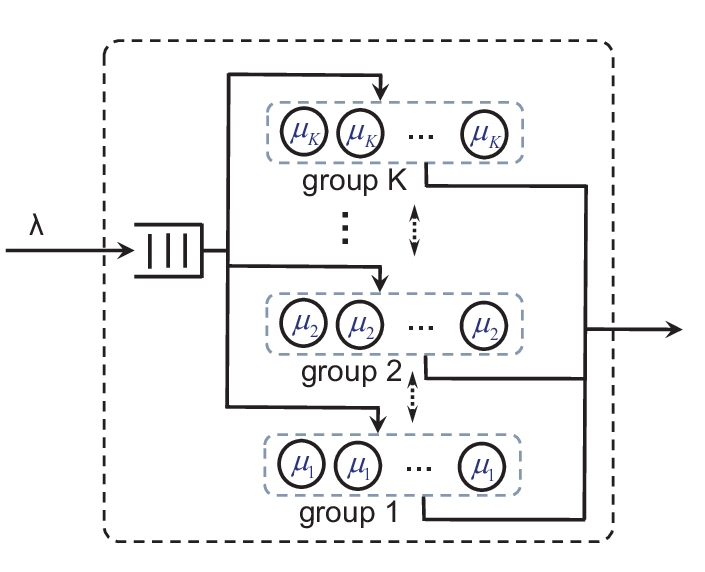
The problem is about the on/off scheduling control of parallel servers in a group-server queue. More details of the problem setting can be referred to (Xia et al 2018) and we give a brief introduction as follows. Consider a group-server queue with a single infinite-size buffer and $K$ groups of parallel servers, as illustrated by Fig. 1. Customers are homogeneous and customer arrival is assumed as a Poisson process with rate $\lambda$. Arriving customers will go to the idle servers at status ‘on’. If all the servers at status ‘on’ are busy, the arriving customer will wait in the buffer. Servers are providing service in parallel and categorized into $K$ groups. Servers in the same group are homogeneous in service rates and cost rates, while those in different groups are heterogeneous. Group $k$ has $M_{k}$ servers with service rate $\mu_{k}$ and cost rate $c_{k}$ per unit of time, $k=1,2,\cdots,K$. Without loss of generality, we assume $\mu_{1}\geq\mu_{2}\geq\dots\geq\mu_{K}$. The system cost includes two parts, the operating cost of servers and the holding cost of customers. The system state $n$ is the number of customers in the system. The state space is denoted as $\mbox{$\cal S$}=\{0,1,2,\dots\}$, which is countably infinite. We can turn on or off servers dynamically to reduce the system average cost. The action is the number of working servers at each group, which is denoted as $a=(a_{1},a_{2},\cdots,a_{K})$, where $a_{k}$ is the number of working servers in group $k$ and $a_{k}\in\{0,1,\cdots,M_{k}\}$. For any state $n\geq 1$, action space $\mathcal{A}(n)$ is a subset of $\{1,\ldots,M_{1}\}\times\{0,\ldots,M_{2}\}\times\cdots\times\{0,\ldots,M_{K}\}$, where $a_{1}\geq 1$ is reasonable to guarantee the system ergodic. Define a stationary policy as $u:=(u(0),u(1),u(2),\dots)$, where $u(n):=(u(n,1),u(n,2),\dots,u(n,K))\in\mathcal{A}(n)$ is the action at state $n$ and $u(n,k)$ is the number of working servers in group $k$ at state $n$. The cost function at state $n$ under policy $u$ is

$$f(n,u):=h(n)+\sum_{k=1}^{K}c_{k}u(n,k),$$

(10)

where $h(n)$ is the holding cost rate at state $n$. The system long-run average cost under policy $u$ is defined as

$$\eta(u)=\lim\limits_{T\rightarrow\infty}\frac{1}{T}\mathbb{E}\left\{\int_{t=0}^{T}f(n(t),u)dt\right\},$$

(11)

where $n(t)$ is the system state at time $t$. The optimal average cost is $\eta^{*}=\inf\limits_{u}[\eta(u)]$. We aim at finding the optimal stationary policy $u^{*}$ which achieves the optimal average cost, i.e., $\eta(u^{*})=\eta^{*}$, where $u^{*}\in\mathcal{U}$ and $\mathcal{U}$ is the stationary policy space. In (Xia et al 2018), it is shown that the optimal policies (if one exists) follow the so called $c/\mu$-rule: Servers in the group with smaller values of $c/\mu$ should be turned on with higher priority. Here, we want to verify that an optimal stationary policy does exist for this problem with countable states.

It is natural to assume that the holding cost $h(n)$ is increasing in $n$; and thus, under optimal policies the queue should be ergodic. So we assume that $\{n(t)\}$ is ergodic (under each policy in $\cal U$) with a unique steady-state distribution $\pi(n,u)$, $n=0,1,\cdots$, $u\in\mbox{$\cal U$}$, and the long-run average (11) does not depend on the initial state.

Since our queue is a birth-death process, we can derive the steady-state distribution as below.

$\displaystyle\pi(n,u)=\frac{1}{1+G(u)}\prod_{l=1}^{n}\frac{\lambda}{u(l)\mu},\qquad n\geq 1,$

(12)

where $\mu=(\mu_{1},\cdots,\mu_{K})^{T}$, and

$$u(l)\mu:=\sum_{k=1}^{K}u(l,k)\mu_{k},$$

(13)

and

$$G(u):=\sum_{n=1}^{\infty}\prod_{l=1}^{n}\frac{\lambda}{u(l)\mu}.$$

(14)

The queue is stable if and only if $G(u)<\infty$ which also indicates

$$\lim\limits_{n\rightarrow\infty}\sum_{m=n}^{\infty}\prod_{l=1}^{m}\frac{\lambda}{u(l)\mu}=0.$$

(15)

The ergodicity of the system under a policy $u$ can indicate a necessary condition: $u(n)\mu\neq 0$ for all $n\geq 1$. The stability of the system can be guaranteed by a sufficient condition: there exists an $\bar{n}$ such that $u(n)\mu>\lambda$ for all $n>\bar{n}$.

For an ergodic policy $u\in\mbox{$\cal U$}$, under suitable condition, the long-run average (11) equals

$$\eta(u)=\sum_{n=0}^{\infty}\pi(n,u)f(n,u).$$

(16)

For the analysis here, we need to make the following assumption:

We use the metric definition (5) to quantify the distance between any two policies $u_{1}$ and $u_{2}$. In what follows, we will prove that when the two policies $u$ and $u^{\prime}$ are infinitely close, their performance measures $\eta(u)$ and $\eta(u^{\prime})$ are also infinitely close to each other. Denote the two policies by $u=(u(0),u(1),\cdots,u(n),\cdots)$ and $u^{\prime}=(u^{\prime}(0),u^{\prime}(1),\cdots,u^{\prime}(n),\cdots)$. By Lemma 1, we assume that

$$u(l)=u^{\prime}(l),~~for~l=0,1,\cdots,n.$$

(17)

which means that $u^{\prime}\in O_{r^{n}}(u)$.

First, we compare the difference of the normalization factors $1+G(u)$ and $1+G(u^{\prime})$ of these two policies. We have

	$\displaystyle\frac{1+G(u)}{1+G(u^{\prime})}$	$\displaystyle=$	$\displaystyle\frac{1+\sum_{m=1}^{\infty}\prod_{l=1}^{m}\frac{\lambda}{u(l)\mu}}{1+\sum_{m=1}^{\infty}\prod_{l=1}^{m}\frac{\lambda}{u^{\prime}(l)\mu}}$		(18)
		$\displaystyle=$	$\displaystyle\frac{\Big(1+\sum_{m=1}^{n}\prod_{l=1}^{m}\frac{\lambda}{u(l)\mu}\Big)+\sum_{m=n+1}^{\infty}\prod_{l=1}^{m}\frac{\lambda}{u(l)\mu}}{\Big(1+\sum_{m=1}^{n}\prod_{l=1}^{m}\frac{\lambda}{u(l)\mu}\Big)+\sum_{m=n+1}^{\infty}\prod_{l=1}^{m}\frac{\lambda}{u^{\prime}(l)\mu}}$
		$\displaystyle=$	$\displaystyle\frac{1+\frac{\sum_{m=n+1}^{\infty}\prod_{l=1}^{m}\frac{\lambda}{u(l)\mu}}{1+\sum_{m=1}^{n}\prod_{l=1}^{m}\frac{\lambda}{u(l)\mu}}}{1+\frac{\sum_{m=n+1}^{\infty}\prod_{l=1}^{m}\frac{\lambda}{u^{\prime}(l)\mu}}{1+\sum_{m=1}^{n}\prod_{l=1}^{m}\frac{\lambda}{u(l)\mu}}}<1+\frac{\sum_{m=n+1}^{\infty}\prod_{l=1}^{m}\frac{\lambda}{u(l)\mu}}{1+\sum_{m=1}^{n}\prod_{l=1}^{m}\frac{\lambda}{u(l)\mu}}$
		$\displaystyle<$	$\displaystyle 1+\sum_{m=n+1}^{\infty}\prod_{l=1}^{m}\frac{\lambda}{u(l)\mu}=1+\delta(n,u),$

where

$$\delta(n,u):=\sum_{m=n+1}^{\infty}\prod_{l=1}^{m}\frac{\lambda}{u(l)\mu}.$$

(19)

Similarly, we can also have

	$\displaystyle\frac{1+G(u)}{1+G(u^{\prime})}$	$\displaystyle=$	$\displaystyle\frac{1+\sum_{m=1}^{\infty}\prod_{l=1}^{m}\frac{\lambda}{u(l)\mu}}{1+\sum_{m=1}^{\infty}\prod_{l=1}^{m}\frac{\lambda}{u^{\prime}(l)\mu}}=\frac{1+\frac{\sum_{m=n+1}^{\infty}\prod_{l=1}^{m}\frac{\lambda}{u(l)\mu}}{1+\sum_{m=1}^{n}\prod_{l=1}^{m}\frac{\lambda}{u(l)\mu}}}{1+\frac{\sum_{m=n+1}^{\infty}\prod_{l=1}^{m}\frac{\lambda}{u^{\prime}(l)\mu}}{1+\sum_{m=1}^{n}\prod_{l=1}^{m}\frac{\lambda}{u(l)\mu}}}$		(20)
		$\displaystyle>$	$\displaystyle\frac{1}{1+\frac{\sum_{m=n+1}^{\infty}\prod_{l=1}^{m}\frac{\lambda}{u^{\prime}(l)\mu}}{1+\sum_{m=1}^{n}\prod_{l=1}^{m}\frac{\lambda}{u(l)\mu}}}>\frac{1}{1+\sum_{m=n+1}^{\infty}\prod_{l=1}^{m}\frac{\lambda}{u^{\prime}(l)\mu}}$
		$\displaystyle>$	$\displaystyle 1-\sum_{m=n+1}^{\infty}\prod_{l=1}^{m}\frac{\lambda}{u^{\prime}(l)\mu}=1-\delta(n,u^{\prime}),$

where

$$\delta(n,u^{\prime}):=\sum_{m=n+1}^{\infty}\prod_{l=1}^{m}\frac{\lambda}{u^{\prime}(l)\mu}.$$

(21)

Therefore, we have

$\displaystyle 1-\delta(n,u^{\prime})<\frac{1+G(u)}{1+G(u^{\prime})}<1+\delta(n,u).$

(22)

Let $\sigma(n,u,u^{\prime})$ be determined by

$$\frac{1+G(u)}{1+G(u^{\prime})}=1+\sigma(n,u,u^{\prime}).$$

(23)

Then,

$$-\delta(n,u^{\prime})<\sigma(n,u,u^{\prime})<\delta(n,u).$$

(24)

With (12), (17), and (23), the steady-state distributions under these two policies $u$ and $u^{\prime}$ have the following relation.

$$\pi(m,u^{\prime})=(1+\sigma(n,u,u^{\prime}))\pi(m,u),\qquad m=0,1,\dots,n.$$

(25)

Next, we study the difference between the associated long-run average costs $\eta$ under policies $u$ and $u^{\prime}$. The cost functions are denoted by $f(m,u)$ and $f(m,u^{\prime})$, respectively. By (10) and (17), we have $f(m,u)=f(m,u^{\prime})$ for $m=0,1,\dots,n$. Therefore, we have

			$\displaystyle\eta(u^{\prime})-\eta(u)$
		$\displaystyle=$	$\displaystyle\sum_{m=0}^{\infty}[\pi(m,u^{\prime})f(m,u^{\prime})-\pi(m,u)f(m,u)]$
		$\displaystyle=$	$\displaystyle\sum_{m=0}^{n}[\pi(m,u^{\prime})f(m,u^{\prime})-\pi(m,u)f(m,u)]+\sum_{m=n+1}^{\infty}[\pi(m,u^{\prime})f(m,u^{\prime})-\pi(m,u)f(m,u)]$
		$\displaystyle=$	$\displaystyle\sum_{m=0}^{n}[\pi(m,u^{\prime})-\pi(m,u)]f(m,u)+\sum_{m=n+1}^{\infty}[\pi(m,u^{\prime})f(m,u^{\prime})-\pi(m,u)f(m,u)].$

Applying (25), we have

$$\eta(u^{\prime})-\eta(u)=\sigma(n,u,u^{\prime})\sum_{m=0}^{n}\pi(m,u)f(m,u)+\sum_{m=n+1}^{\infty}[\pi(m,u^{\prime})f(m,u^{\prime})-\pi(m,u)f(m,u)].$$

(26)

Now we are ready to prove the continuity of $\eta(u)$ in the metric space $\cal U$ with metric (5). With (15), we have

$$\lim\limits_{n\rightarrow\infty}\delta(n,u)=0,\qquad\lim\limits_{n\rightarrow\infty}\delta(n,u^{\prime})=0.$$

Let $\epsilon>0$ be any small number. Under Assumption 1, by the uniformity of $G(u)$ in (14) and (15), there exists a large integer $N_{1}$ such that if $n>N_{1}$, we have $\delta(n,u)<\epsilon$ for any $u\in\mbox{$\cal U$}$. By (24), we have

$$|\sigma(n,u,u^{\prime})|<\epsilon,\quad\forall u,u^{\prime}\in\mbox{$\cal U$}.$$

Next, because (16) converges, there is a large integer $N_{2}$ such that

$$\Big|\sum_{m=0}^{n}\pi(m,u)f(m,u)\Big|<|\eta(u)|+1,\quad\forall n>N_{2}.$$

Furthermore, under Assumption 1, by the uniformity of the convergence of (16), there is a large integer $N_{3}$ such that

$$\Big|\sum_{m=n+1}^{\infty}[\pi(m,u^{\prime})f(m,u^{\prime})-\pi(m,u)f(m,u)]\Big|<2\epsilon,\quad\forall n>N_{3}\ {\rm and}\ u,u^{\prime}\in\mbox{$\cal U$}.$$

Finally, let $N^{*}:=\max\{N_{1},N_{2},N_{3}\}$. Then, by (26) and Lemma 1, we have

	$\displaystyle|\eta(u)-\eta(u^{\prime})|$	$\displaystyle\leq$	$\displaystyle|\sigma(n,u,u^{\prime})|\Big|\sum_{m=0}^{n}\pi(m,u)f(m,u)\Big|+\Big|\sum_{m=n+1}^{\infty}[\pi(m,u^{\prime})f(m,u^{\prime})-\pi(m,u)f(m,u)]\Big|$		(27)
		$\displaystyle<$	$\displaystyle[|\eta(u)|+3]\epsilon,\ \ \ \ {\rm for\ all\ }u^{\prime}\in O_{r^{N^{*}}}(u).$

Since $\eta(u)$ is bounded, we conclude that $\eta(u)$ is continuous at $u$ in the metric space. Therefore, the existence of optimal stationary policy $u^{*}$ for this $c/\mu$-rule problem directly follows by Theorem 1. $\Box$

References

- Borkar (1989) Borkar, V. S. (1989). Control of Markov chains with long-run average cost criterion: The dynamic programming equations. SIAM Journal on Control and Optimization, Vol. 27, pp. 642-657.
- Borkar (1994) Borkar, V. S. (1994). Ergodic control of Markov chains with constraints–the general case. SIAM Journal on Control and Optimization, Vol. 32, pp. 176-186.
- Bertsekas (2012) Bertsekas, D. P. (2012). Dynamic Programming and Optimal Control–Vol.2, 4th Edition. Boston: Athena Scientific.
- Cao and Xie (2015) Cao, P. and Xie, J. (2015). A new condition for the existence of optimal stationary policies in denumerable state average cost continuous time Markov decision processes with unbounded cost and transition rates. arXiv:1504.05674.
- Cavazos-Cadena (1991) Cavazos-Cadena, R. Recent results on conditions for the existence of average optimal stationary policies. Annals of Operations Research, Vol. 28, pp. 3-27.
- Cavazos-Cadena and Sennott (1992) Cavazos-Cadena, R. and Sennott, L. I. (1992). Comparing recent assumptions for the existence of optimal stationary policies. Operations Research Letters, Vol. 11, pp. 33-37.
- Feinberg and Lewis (2007) Feinberg, E. A. and Lewis, M. E. (2007). Optimality inequalities for average cost Markov decision processes and the stochastic cash balance problem. Mathematics of Operations Research, Vol. 32, pp. 769-785.
- Golubin (2003) Golubin, A. Y. (2003). A note on the convergence of policy iteration in Markov decision processes with compact action spaces. Mathematics of Operations Research, Vol. 28, pp. 194-200.
- Guo and Rieder (2006) Guo, X. and Rieder, U. (2006). Average optimality for continous-time Markov decision processes in Polish spaces. Annals of Applied Probability, Vol. 16, pp. 730-756.
- Guo and Hernández-Lerma (2009) Guo, X. and Hernández-Lerma, O. (2009). Continuous-Time Markov Decision Processes. Springer.
- Lasserre (1988) Lasserre, J. B. (1988). Conditions for existence of average and Blackwell optimal stationary policies in denumerable Markov decision processes. J. Math. Anal. Appl., Vol. 136, pp. 479-490.
- Meyn (1997) Meyn, S. (1997). The policy iteration algorithm for average reward Markov decision processes with general state space. IEEE Transactions on Automatic Control, Vol. 42, pp. 1663-1680.
- Meyn (1999) Meyn, S. (1999). Algorithms for optimization and stabilization of controlled Markov chains. Sadhana, Vol. 24, pp. 339-367.
- Hernández-Lerma (1991) Hernández-Lerma, O. (1991). Average optimality in dynamic programming on Borel spaces. Systems and Control Letters, Vol. 17, pp. 237-242.
- Hernández-Lerma and Lasserre (1996) Hernández-Lerma, O. and Lasserre, J. B. (1996). Discrete-Time Markov Control Processes: Basic Optimality Criteria. Springer, New York.
- Hernández-Lerma and Lasserre (1999) Hernández-Lerma, O. and Lasserre, J. B. (1999). Further Topics on Discrete-Time Markov Control Processes. Springer, New York.
- Puterman (1994) Puterman, M. L. (1994). Markov Decision Processes: Discrete Stochastic Dynamic Programming. New York: John Wiley & Sons.
- Ross (1971) Ross, S. M. (1971). On the nonexistence of -optimal randomized stationary policies in average cost Markov decision models. The Annals of Math. Statistics, Vol 42, pp. 1767-1768.
- Sennott (1986) Sennott, L. I. (1986). A new condition for the existence of optimum stationary policies in average cost Markov decision processes. Operations Research Letters, Vol. 5, pp. 17-23.
- Sennott (1989) Sennott, L. I. (1989). Average cost optimal stationary policies in infinite state Markov decision processes with unbounded costs. Operations Research, Vol. 37, pp. 626-633.
- Sennott (1999) Sennott, L. I. (1999). Stochastic Dynamic Programming and the Control of Queueing Systems. New York: John Wiley & Sons.
- Xia et al (2018) Xia, L., Zhang, Z. G., Li, Q., and Glynn, P. W. (2018). A c/-rule for service resource allocation in group-server queues. arXiv:1807.05367 [math.OC].