se counter=example]example[2][]title=Example \thetcbcounter: #2,#1

Modes of Homogeneous Gradient FlowsThanks: Ido would like to thank Prof. Andrea Bertozzi for the opportunity of studying in mathematics science department, UCLA in general and for helpful conversations, related to this work, in particular. We thank Prof. Ronen Talmon for stimulating discussions. And we also would like to thank Shachar Praisler for his helpfull advice. Funding: This work was supported by the European Union’s Horizon 2020 research and innovation programme under the Marie Skłodowska-Curie grant agreement No. 777826 (NoMADS). GG acknowledges support by the Israel Science Foundation (Grant No. 534/19) and by the Ollendorff Minerva Center.

Ido Cohen Thanks: Electrical Engineering Department at the Technion – Israel Institute of Technology (idoc@campus.technion.ac.il,pavel@ee.technion.ac.il,guy.gilboa@ee.technion.ac.il). Omri Azencot Thanks: Department of Mathematics, University of California Los Angeles (azencot@math.ucla.edu). Pavel Lifshits ²²footnotemark: 2 Guy Gilboa ²²footnotemark: 2

August 11, 2026

Abstract

Finding latent structures in data is drawing increasing attention in diverse fields such as image and signal processing, fluid dynamics, and machine learning. In this work we examine the problem of finding the main modes of gradient flows. Gradient descent is a fundamental process in optimization where its stochastic version is prominent in training of neural networks. Here our aim is to establish a consistent theory for gradient flows $\psi_{t}=P(\psi)$ , where $P$ is a nonlinear homogeneous operator. Our proposed framework stems from analytic solutions of homogeneous flows, previously formalized by Cohen-Gilboa, where the initial condition $\psi_{0}$ admits the nonlinear eigenvalue problem $P(\psi_{0})=\lambda\psi_{0}$ . We first present an analytic solution for DMD (DMD) in such cases. We show an inherent flaw of DMD, which is unable to recover the essential dynamics of the flow. It is evident that DMD is best suited for homogeneous flows of degree one. We propose an adaptive time sampling scheme and show its dynamics are analogue to homogeneous flows of degree one with a fixed step size. Moreover, we adapt DMD to yield a real spectrum, using symmetric matrices. Our analytic solution of the proposed scheme recovers the dynamics perfectly and yields zero error. We then proceed to show that in the general case the orthogonal modes $\{\phi_{i}\}$ are approximately nonlinear eigenfunctions $P(\phi_{i})\approx\lambda_{i}\phi_{i}$ . We formulate Orthogonal Nonlinear Spectral decomposition (OrthoNS), which recovers the essential latent structures of the gradient descent process. Definitions for spectrum and filtering are given, and a Parseval-type identity is shown. Experimental results on images, show the resemblance to direct computations of nonlinear sepctral decomposition. A significant speedup (by about two orders of magnitude) is achieved for this application using the proposed method.

Keywords— nonlinear decomposition, dynamic mode decomposition, homogeneous operators, gradient flows, nonlinear spectral theory.

1 Introduction

Finding latent structures in data is a fundamental task in diverse fields. Some canonical examples are wavelets and dictionaries in image and signal processing [1, 2, 3], dynamic modes in fluid dynamics analysis [4, 5], and dimensionality reduction and invariant representations in machine learning [6, 7, 8]. Understanding the latent structures allows to better model and to simplify the problem at hand, facilitating solutions for broad applications such as denoising, prediction, and classification [9]. These structures are formulated differently in different disciplines. For example, in image processing, the structures can be formed via repetitive patches in different scales [10], while in signal processing they can be a sum of audio frequencies, or of nonlinear eigenfunctions [11, 12]. In fluid dynamics the structures are represented as a sum of modes [13], and in machine learning they might be based on the recurrence of words [14]. Despite this diversity, different techniques from different disciplines typically share similar fundamental principles.

Gradient descent flow is a central process in control [15] and in machine learning [16], where it is common to solve optimization problems. Thus, analysing the gradient flow process draws attention in these areas and plays an important role, particularly when the cost function is non-convex [17, 18], or when a model for a dynamical system is investigated [19].

In this work, we propose a method to analyze latent structures of certain common gradient decent flows by using DMD (DMD). DMD is often used today in fluid dynamics for finding the main modes of a dynamical system. DMD is an effective tool for analyzing nonlinear flows [20, 21, 22]. It is an approximation of the linear infinite-dimensional Koopman operator [13, 23, 24]. We focus on a gradient flow of a homogeneous functional $R$ ,

\psi_{t}=P(\psi),\hskip 18.49988ptP=-\partial R_{\psi},\hskip 9.24994pt\psi(t=0)=f,

where $P$ is a homogeneous operator (typically with order of homogeneity in the range $[0,1]$ ). When a norm or a semi-norm is minimized, in its standard or quadratic form, we obtain such flows. As shown in [25], the solution of this equation reaches its steady state in finite time (for order strictly less than one). Moreover, the solution is separable (in time and space) if $f$ is a (nonlinear) eigenfunction of $P$ , i.e. $f$ solves the nonlinear eigenvalue problem $P(f)=\lambda\cdot f$ . Precisely, the solution is a multiplication between the initial condition $f$ and a time dependant function $a(t)$ : $\psi(t)=a(t)\cdot f$ , where $a(t)$ has a closed form solution, which depends on the degree of the homogeneity of $P$ and on the eigenvalue $\lambda$ .

With the purpose of better understanding DMD of homogeneous flows, we examine the analytic solutions of such flows. We present a closed form solution of DMD in these cases and discover an inherent flaw. Specifically, for general homogeneous flows, DMD can not recover the extinction time of the dynamics, and it induces a significant reconstruction error. Our analysis further shows that DMD is well-suited for flows with one-homogeneous operators. Consequently and inspired by [26], we suggest a new scheme which employs an adaptive time sampling instead of a fixed time step size. We show that our temporal re-scaling is equivalent to evolving a one-homogeneous flow. With this adaptation, DMD is able to recover homogeneous flows of order $[0,1]$ . In the general case, we additionally obtain a much better mode recovering scheme which captures the dynamics of the flow well. Next, we show that the obtained modes approximate nonlinear eigenfunctions, allowing us to link DMD to nonlinear spectral theory. In summary, our analysis and results yield a new and simple spectral decomposition framework. Our work generalizes previous studies which directly formulated nonlinear spectral representations based on total-variation [27, 28] and one-homogeneous functionals [11, 29] by applying (weak) time-derivatives to the solution of a gradient flow. It is also related to previous research in which signals were analyzed by their decay profile, as shown in [30, 31].

Main contributions and structure of paper

Our contributions can be summarized as follows:

1.

It is shown that DMD is not effective for homogeneous flows with homogeneity different than one. This inherent limitation is formulated by what we term the DMD paradox, where as the step-size decreases, the standard DMD-error approaches zero, whereas the reconstruction error has a strictly positive lower bound.
2.

We propose a temporal re-parametrization scheme of the data sampling. We study cases with an analytic solution, and we show that our re-parametrization yields a single mode in DMD which can be perfectly reconstructed. Finally, the relation to an analogue one-homogeneous flow is shown.
3.

The temporal re-parametrization of the data is generalized to arbitrary step sizes and to any homogeneity. We term this adaptation as the blind homogeneity normalization, where the blind is twofold, neither the operator nor the temporal sampling are known.
4.

We adapt the DMD algorithm to real valued spectrum systems, common in smoothing-type (non-oscillatory) flows. We refer to it as SDMD (SDMD).
5.

We introduce a new discrete analysis and synthesis framework of signals related to homogeneous flows of homogeneity order in $[0,1]$ . Our framework is based on orthogonal modes which approximate nonlinear eigenfunctions. We thus refer to it as Orthogonal Nonlinear Spectral decomposition. We numerically compare our decomposition to the method in [25], and we show that our scheme is simpler, more general, and it is $1-2$ orders of magnitude faster than [25].

The paper is organized as follows. We briefly recall the necessary mathematical definitions and previous results in Sec. 2. In Sec. 3 a closed form solution for DMD in certain cases is given and the paradox for homogeneous flows is stated. Our solution is proposed (in non-blind and blind versions) and analyzed. The OrthoNS representation is formalized. In addition, we introduce the SDMD method such that DMD is based on a symmetric matrix. In Sec. 4 we demonstrate SDMD, then show the main modes of two gradient descent flows with respect to the $p-$ Dirichlet energy ( $p=1.01$ and $p=1.5$ ), when initialized with a square peak. Filtering of signals by OrthoNS are presented along with a comparison to [25]. We conclude our work and discuss future directions in Sec. 5.

2 Preliminaries

Let $\mathcal{H}$ be a real Hilbert space equipped with a norm $\|\cdot\|$ . Typically, in a discrete setting, we have $\mathcal{H}=\mathbb{R}^{M}$ and a Euclidean norm. A common optimization problem, given some data $f\in\mathcal{H}$ , is to seek a solution $\psi\in\mathcal{H}$ which minimizes

G(\psi)=F(\psi,f)+R(\psi),

(1)

where $F:\mathcal{H}\to\mathbb{R}^{+}$ is a fidelity (or data) term and $R:\mathcal{H}\to\mathbb{R}^{+}$ is a regularization term. In the most simple case, the denoising problem, $F$ can be the square $\ell^{2}$ norm and $R$ is the Dirichlet energy or, alternatively, the total-variation energy (yielding Tikhonov [32] or ROF [33] models, respectively).The solution $\psi^{*}=\argmin_{\psi}G(\psi,f)$ is a compromise between the noisy data and a regular solution. In this paper we focus on regularization terms which are absolutely $p$ -homogeneous functionals, admitting

R(a\cdot\psi)=\absolutevalue{a}^{p}\cdot R(\psi),

(2)

for any $a\in\mathbb{R}$ . One can obtain a local minimizer by evolving a gradient descent process with respect to the total energy $G$ . In the denoising case, when the fidelity is a simple Euclidean norm, an alternative solution is to evolve gradient descent with respect to $R$ only and to stop at a certain desired time-point in the process. Given $-P=\partial_{\psi}R(\psi)$ the gradient descent flow is

\psi_{t}=-\partial_{\psi}R(\psi)=P(\psi),\hskip 9.24994pt\psi(0)=f,

(3)

where $\psi_{t}$ is the time derivative of the solution, and the initial condition is $f$ . The operator $P$ is $(p-1)$ -homogeneous,

P(a\cdot\psi)=a\absolutevalue{a}^{p-2}\cdot P(\psi),\,\,\,a\in\mathbb{R}.

(4)

We refer to Eq. (3) as a homogeneous flow.

2.1 The p-Framework

Based on nonlinear spectral representations of one-homogeneous functionals [28, 11, 29], an extension to functionals of homogeneity $p\in(1,2)$ was proposed in [25]. As in previous studies, the representation is based on manipulating a gradient flow process. In [25] the flow of Eq. (3) was analyzed. A special case was investigated more deeply, where the solution of Eq. (3) admits a separation of variables,

\psi(t)=a(t)\cdot f.

(5)

In this case the initial condition $f$ remains unchanged (spatially), while its scale changes over time. This form of solution is obtained iff $f$ is a (nonlinear) eigenfunction of $P$ , i.e. it solves the following nonlinear eigenvalue problem,

P(f)=\lambda\cdot f,

(EF)

where $\lambda\in\mathbb{R}$ is the eigenvalue. The function $a(t)$ can be viewed as a decay profile. The decay depends on the eigenvalue and the order of homogeneity, and it is given by,

a(t)=\left[(1+(2-p)\lambda\cdot t)^{+}\right]^{\frac{1}{2-p}},

(6)

where $(a)^{+}=\max\{0,a\}$ . We note that the operator $-P(\cdot)$ is assumed to be maximally monotone. Therefore, its spectrum is non-positive, where $\lambda\leq 0$ . The decay profile (6) has thus a finite support in time. The solution reaches its steady state in finite time, termed as the extinction time. The extinction time is given by

T=-\frac{1}{\lambda(2-p)}.

(7)

It can also be shown that under mild conditions on $P$ the flow (3) converges in finite time for arbitrary initial conditions. A particular example for $R$ is the $p$ -Dirichlet energy, thoroughly studied in the context of image processing by Kuijper (c.f. [34]),

R(\psi)=J_{p}(\psi)=\frac{1}{p}\norm{\nabla\psi}^{p}.

(8)

Kuijper suggested to use the respective gradient descent flow as a nonlinear scale space,

\psi_{t}=\Delta_{p}\psi,\hskip 9.24994pt\psi(0)=f,

(p-Flow)

where $\Delta_{p}(\cdot)$ is the $p$ -Laplacian operator,

\Delta_{p}(\psi)=\divergence{\{\abs{\nabla\psi}^{p-2} \nabla\psi\}}.

(9)

The $p$ -Dirichlet is an absolutely $p$ -homogeneous functional and the $p$ -Laplacian operator is coercive and maximally monotone. Therefore, the discussion above is valid for (p-Flow) for $p\in[1,2)$ . If the initial condition, $f$ , admits (EF), for $P=\Delta_{p}$ , then the solution of (p-Flow) is given by Eqs. (5), (6) and the extinction time is (7). In Fig. 1 the process (p-Flow) is depicted for $p=1.5$ .

2.2 Time discretisation of homogeneous flows

The explicit scheme of Eq. (3) reads,

\psi_{k+1}=\psi_{k}+P(\psi_{k})\cdot dt_{k},\hskip 9.24994pt\psi_{0}=f.

(10)

If the initial condition, $f$ , is an eigenfunction (EF), then the solution of (10) is

\psi_{k}=a_{k}\cdot f,\hskip 9.24994pta_{k}\in\mathbb{R}.

(11)

For $(p-1)$ -homogeneous operator $P$ the recurrence relating $a_{k+1}$ to $a_{k}$ is [26]

a_{k+1}=a_{k}\left(1+\absolutevalue{a_k}^{p-2}\lambda dt_{k}\right),\hskip 9.24994pta_{0}=1.

(12)

In standard explicit implementations one needs to regularize the functional (and respective operator) to obtain a practical step size (dictated by the CFL condition). This yields either very small step-sizes or strong deviation from the original flow. In [26] an alternative scheme was proposed which uses an adaptive step size. We will later see how this scheme directly connects to our proposed time re-sampling.

Adaptive step size policy

In [26] an adaptive step-size policy was proposed for the explicit scheme (10), given by

dt_{k}=-\frac{\langle P(\psi_{k}),\psi_{k}\rangle}{\norm{P(\psi_k)}^{2}}\cdot\delta,\hskip 9.24994pt\delta\in(0,2),

(13)

where $\delta$ is a free parameter controlling the speed of the process. It was shown that the scheme is stable for arbitrary $f$ and $\delta\in(0,2)$ . For $f$ which is an eigenfunction the solution is Eq. (11), where

a_{k}=(1-\delta)^{k}.

(14)

We note that although [26] focused on the $p$ -Laplacian flow, the above results are valid for any homogeneous operator of order between zero and one which is coercive and maximally monotone. See a recent general study [35] on the relations between statistical estimators of order $p$ and their respective PDE’s in the limit.

2.3 DMD (DMD)

DMD [13] is an analysis tool used to recover the main spatial structures in a fluid flow. Its stages are detailed in Algorithm 1. We first present the rationale, notations and definitions of the algorithm. Vectors are denoted by boldface and matrices by capital letters. We depict here the general case, however, in the following sections we focus on the representation of the data matrices over the real field.

Matrices of the dynamics

The data consists of $N+1$ snapshots in time of a flow $\bm{\psi_{k}}\in\mathbb{R}^{M}$ , $\{\bm{\psi_{k}}\}_{k=0}^{N}$ . We construct two $M\times N$ matrices as follows,

\begin{split}\Psi_{0}^{N-1}&=\begin{bmatrix}\bm{\psi_{0}}&\cdots&\bm{\psi_{N-1}}\end{bmatrix}\\ \Psi_{1}^{N}&=\begin{bmatrix}\bm{\psi_{1}}&\cdots&\bm{\psi_{N}}\end{bmatrix}.\end{split}

(15)

Dimensionality reduction

A main assumption of DMD is that the data can be well represented in a lower dimensional space. To reduce the dimensionality we need to find the singular vectors that span the columns of $\Psi_{0}^{N-1}$ . SVD (SVD) is used to find these vectors since the matrix $\Psi_{0}^{N-1}$ is not square. This decomposition is an extension of the eigenvector problem for non square matrices (for details see e.g. [36] Ch. I.8), and it is given by

\Psi_{0}^{N-1}=U\Sigma V^{*}.

(16)

The superscript ^∗ denotes the conjugate transpose. The matrix $U$ is an $M\times N$ orthogonal matrix ( $U^{*}U=I_{N\times N}$ ), $V$ is an $N\times N$ orthogonal matrix ( $V^{*}V=I_{N\times N}$ ), and $\Sigma$ is an $N\times N$ diagonal matrix, where the entries on the diagonal are the singular values.

We denote by $U_{r}$ and $V_{r}$ the submatrices, containing the first $r$ columns of $U$ and $V$ , respectively ( $r\ll M$ ). $\Sigma_{r}$ is the a submatrix of $\Sigma$ , containing the $r\times r$ left upper entries of $\Sigma$ . The dimensionality reduction of the data is obtained by setting

\begin{split}X&=U_{r}^{*}\Psi_{0}^{N-1},\hskip 18.49988ptY=U_{r}^{*}\Psi_{1}^{N}.\end{split}

(17)

The $k$ th column in the matrix $X$ , denoted by ${\bm{x_{k}}}$ , is the lower dimensional representation of the $k$ th snapshot, ${\bm{\psi_{k}}}$ , i.e. ${\bm{x_{k}}}=U_{r}^{*}{\bm{\psi_{k}}}$ . Note that the columns of $U_{r}$ are a basis of a linear space and the entries of $\bm{x_{k}}$ can be viewed as coordinates of the snapshot $\bm{\psi_{k}}$ in that space.

Mode, spectrum and coordinates calculation

In the lower-dimensional space we seek a linear mapping $F$ from $X$ to $Y$ that minimizes the Frobenius norm

ERR_{DMD}=\min_{F}\norm{Y-FX}^{2}_{\mathcal{F}}.

(18)

The solution of this optimization problem is given by,

F=YX^{T}\cdot\left(XX^{T}\right)^{-1}=U_{r}^{*}\Psi_{1}^{N+1}V_{r}\Sigma_{r}^{-1},

(19)

termed as the DMD matrix. Then, the $k+1$ th sample can be expressed as

\bm{x_{k}}\approx F\cdot\bm{x_{k-1}}.

(20)

We denote by $\approx$ the linear, dimensionality-reduced approximation of the dynamical system. The linear mapping approximation, $F$ , minimizes the Frobenius norm of the error with respect to the first $r$ dominant singular vectors of the data. Assuming the matrix $F$ is full rank, we can reformulate Eq. (20) as

\bm{x_{k}}\approx WDW^{*}\cdot\bm{x_{k-1}},

(21)

where $D$ is a diagonal matrix containing the eigenvalues of $F$ , and the matrix $W$ contains the corresponding eigenvectors.

Reconstructing the Dynamics

Discrete time setting

We can reconstruct the dynamics projected on the lower dimensional space, e.g. the initial condition is reconstructed by $\bm{\tilde{\psi}_{0}}=U_{r}\bm{x_{0}}$ . More generally, to reconstruct a snapshot at stage $k$ we can apply the mapping $F$ $k$ times,

\begin{split}\bm{\tilde{\psi}}_{k}=&U_{r}\cdot F^{k}\bm{x_{0}}=U_{r}\cdot WD^{k}W^{*}U_{r}^{*}\bm{\psi}_{0}\\ =&U_{r}\cdot\begin{bmatrix}\bm{w_{1}}&\cdots&\bm{w_{r}}\end{bmatrix}\cdot\begin{bmatrix}\mu_{1}^{k}&&0\\ &\ddots&\\ 0&&\mu_{r}^{k}\end{bmatrix}\cdot\begin{bmatrix}\bm{w_{1}}^{*}\\ \vdots\\ \bm{w_{r}}^{*}\end{bmatrix}\cdot U_{r}^{*}\bm{\psi}_{0}=\sum_{i=1}^{r}\alpha_{i}\mu_{i}^{k}\bm{\phi_{i}},\end{split}

(22)

where the modes, $\{\bm{\phi_{i}}\}_{i=1}^{r}$ , and coordinates $\{\alpha_{i}\}_{i=1}^{r}$ are

\bm{\phi_{i}}=U_{r}\bm{w_{i}},\hskip 9.24994pt\alpha_{i}={\bm{w_{i}}}^{*}U_{r}^{*}\psi_{0},

and $\{\mu_{i}\}_{i=1}^{r}$ are the eigenvalues of the matrix $F$ (the spectrum).

Algorithm 1 Standard DMD [13]

1: Inputs:

2: Data sequence

\{{\bm{\psi}_{k}}\}_{0}^{N}

3: Arrange the data into the matrices

\Psi_{0}^{N-1}

and

\Psi_{1}^{N}

according to Eq. (15).

4: Compute the SVD (SVD) of

\Psi_{0}^{N-1}

(see [37]) to the multiplication in Eq. (16).

5: Dimensionality reduction. Reformulate the data matrices,

\Psi_{0}^{N-1},\,\Psi_{1}^{N}

(denoted by

X

and

Y

, respectively) with the first

r

singular vectors from the matrix,

U

, Eq. (17).

6: Find the optimal linear mapping,

F

, between

X

and

Y

in the sense of Eq. (18). The solution is given by Eq. (19).

7: Under the assumption that

F

is a full rank matrix, compute eigenvalues

\mu

and right eigenvectors

\bm{v}

F

, the corresponding modes

\bm{\phi}

, and the corresponding coordinates

\alpha

F\bm{w}=\mu\bm{w},\hskip 9.24994pt\bm{\phi}\triangleq U_{r}\bm{w},\hskip 9.24994pt\alpha\triangleq\bm{w}^{*}U_{r}^{*}\bm{\psi_{0}}.

(23)

8: Outputs:

\{\mu_{i},\bm{\phi_{i}},\alpha_{i}\}_{1}^{r}

Note that, the linear mapping from $\tilde{\psi}_{k}$ to $\tilde{\psi}_{k+1}$ , denoted by $A$ is give by,

A=U_{r}\cdot F\cdot U_{r}^{*}.

(24)

This mapping can be interpreted as a linear approximation of the dynamical system. The modes $\{\phi_{i}\}$ are the right eigenvectors of the matrix $A$ and the corresponding eigenvalues are $\{\mu_{i}\}$ . For reconstruction, we define the (time-discrete) reconstruction error, $ERR^{d}_{Rec}$ , as

ERR_{Rec}^{d}=\sum_{k=0}^{N}\norm{\bm{\tilde{\psi}_k}-\bm{\psi_k}}^{2},

(25)

where $\bm{\tilde{\psi}_{k}}$ is defined in Eq. (22).

Continuous time setting

One can expand the reconstruction, Eq. (22), to the continuous time setting. The discrete reconstruction is a sampling of a continuous exponential function, therefore, with the identity,

\mu_{i}=e^{\tilde{\mu}_{i}dt},

where $dt$ is the sampling time step Thus, in the time continuous setting, the dynamics reconstruction and the corresponding error take the form,

\tilde{\psi}(t)=\sum_{i=1}^{r}\alpha_{i}\bm{\phi_{i}}e^{\tilde{\mu}_{i}t},\hskip 9.24994pt\tilde{\mu}_{i}=\frac{\ln(\mu_i)}{dt},\hskip 9.24994ptERR_{Rec}^{c}=\int(\tilde{\psi}(t)-\psi(t))^{2}dt.

(26)

We would like also to consider the limit case, as the step size between consecutive snapshots, $dt$ , approaches zero. In that case, the eigenvalue $\tilde{\mu}_{i}$ is the limit of the quotient written above.

We note that this is the classical algorithm and several variations and extensions were further proposed. It was shown in [38] that DMD is sensitive to noisy data . Specifically, the spectrum estimation is systematically biased in the presence of noise. This bias is not relaxed when more data is gathered [39]. The effect of small sensor noise on DMD and on the Koopman expansion was studied and characterized in [40]. Several attempts have been made to remove this bias. Dawson et al. proposed the forward and backward dynamics to reduce the noise [41]. Hemati et al. formulated the problem as a total least squares optimization [39]. A variational approach was proposed in [42]. The authors in [43, 44] used Kalman filters to cope with the noise. Williams et al. [45] suggested to extend the basis of the sampled data snapshots, while [46] uses deep learning to learn the basis dictionary of the operator. More recent approaches harness the benefits of neural networks to propose effective Koopman-based designs [47].

3 DMD for homogeneous and symmetric flows

This section presents the main novelties of the paper. DMD is analyzed for homogeneous flows, its flaws are exposed and a solution is presented in the form of a time re-sampling scheme. For non-oscillatory flows we propose SDMD. Finally, we show connections of the modes to nonlinear eigenfunctions and propose the OrthoNS analysis and synthesis framework.

3.1 DMD for homogeneous flows

There are two prominent assumptions in DMD; first, the dynamics can be represented linearly in a lower dimensional space; second, the data is sampled uniformly in time. These assumptions allow us to interpret the system as a linear one [13] and to consider DMD as an exponential data fitting algorithm [20]. Thus, the finite extinction time of homogeneous flows is inherently hard to model in this framework. In what follows, we show the inconsistency and error of DMD applied to flows initiated with eigenfunctions.

3.1.1 Closed from solution of DMD

We begin by computing the DMD modes of the homogeneous flow, Eq. (3), when the initial condition is an eigenfunction. Let us recall that the solution is Eq. (5). Therefore, by sampling this solution with respect to time (with a fixed step size) we get

\psi_{k}=a_{k}\cdot f,\hskip 9.24994pta_{k}\in\mathbb{R},\,a_{0}=1.

(27)

Therefore, the data matrices $\Psi_{1}^{N}$ and $\Psi_{0}^{N-1}$ (Eq. (15)) are in the form of

\Psi_{1}^{N}=f\cdot\left({\bm{a}_{1}^{N}}\right)^{T},\hskip 9.24994pt\Psi_{0}^{N-1}=f\cdot\left({\bm{a}_{0}^{N-1}}\right)^{T},

(28)

where $\bm{a}_{k}^{m}=\begin{bmatrix}a_{k}&\cdots&a_{m}\end{bmatrix}^{T}$ . The following Lemma formulates an analytic solution of the classical DMD for these cases.

Lemma 1 (Analytic solution).

Let the dynamical system be Eq. (3) and the initial condition $f$ is an eigenfunction per Eq. (EF). We obtain the following analytic solution and error for classical DMD, Algo. 1, for $r=1$ :

\mu=\frac{\langle\bm{a}_{1}^{N},\bm{a}_{0}^{N-1}\rangle}{\norm{\bm{a}_0^{N-1}}^{2}},\hskip 9.24994pt\phi=\frac{f}{\norm{f}},\hskip 9.24994pt\alpha=\norm{f}.

(29)

The DMD error (Eq. (18)) is

ERR_{DMD}=\norm{\bm{a}_1^{N}}^{2}-\frac{\langle\bm{a}_{1}^{N},\bm{a}_{0}^{N-1}\rangle^{2}}{\norm{\bm{a}_0^{N-1}}^{2}},

(30)

where $\bm{a}_{0}^{N}$ and $\bm{a}_{1}^{N+1}$ are defined in (28). For $r>1$ the solution does not exist.

Proof.

The data matrix $\Psi_{0}^{N-1}$ (in Eq. (28)) can be reformulated as

\Psi_{0}^{N-1}=U\cdot\Sigma\cdot V^{*}=\frac{f}{\norm{f}}\cdot\norm{f}\norm{\bm{a}_0^{N-1}}\cdot\frac{\bm{a}_{0}^{N-1}}{\norm{\bm{a}_0^{N-1}}}.

The SVD of this matrix is $\Psi_{0}^{N-1}=U\Sigma V^{*}$ where, $U$ is the column vector ${f}/{\norm{f}}$ concatenated by a zero matrix of size ( $M\times(N-1)$ ), $\Sigma$ is $N\times N$ matrix with zeros everywhere except the entry $(1,1)$ where $\Sigma(1,1)=\norm{f}\norm{\bm{a}_0^{N-1}}$ , and $V$ is the column vector ${\bm{a}_{0}^{N-1}}/{\norm{\bm{a}_0^{N-1}}}$ concatenated by a zero matrix of size ( $N\times(N-1)$ ). More formally,

U=\begin{bmatrix}\frac{f}{\norm{f}}&{\bm{0}}&\cdots&{\bm{0}}\end{bmatrix},\,\Sigma=diag\left(\begin{bmatrix}\norm{f}\norm{\bm{a}_0^{N-1}}&0&\cdots&0\end{bmatrix}\right),\,V=\begin{bmatrix}\frac{\bm{a}_{0}^{N-1}}{\norm{\bm{a}_0^{N-1}}}&{\bm{0}}&\cdots&{\bm{0}}\end{bmatrix},

where $U\in\mathbb{R}^{M\times N}$ , $\Sigma\in\mathbb{R}^{N\times N}$ , $V\in\mathbb{R}^{N\times N}$ , and ${\bm{0}}$ is a column zero vector in $\mathbb{R}^{M}$ or $\mathbb{R}^{N}$ . If $r=1$ then $U_{1},\,V_{1}$ are vectors and $\Sigma_{1}$ is a scalar, where they accurately reconstruct $\Psi_{0}^{N-1}$ . This is an expected result since the rank of $\Psi_{0}^{N-1}$ is one. Consequently, $Y$ and $X$ are the following vectors,

Y=U_{1}^{*}\cdot\Psi_{1}^{N}=\norm{f}{\bm{a}_{1}^{N}},\hskip 9.24994ptX=U_{1}^{*}\cdot\Psi_{0}^{N-1}=\norm{f}{\bm{a}_{0}^{N-1}}.

The DMD matrix becomes a scalar, $\mu$ , which minimizes the following term

\begin{split}\mu_{min}=\arg\min_{\mu}\{\norm{Y-\mu X}_{F}^{2}\}=\arg\min_{\mu}\{\norm{\bm{a}_1^N-\mu\bm{a}_0^{N-1}}^{2}\}=\frac{\langle\bm{a}_{1}^{N},\bm{a}_{0}^{N-1}\rangle}{\norm{\bm{a}_0^{N-1}}^{2}}.\end{split}

The eigenvector is $v=1$ . Using the above results and (23), (18) yields (29) and (30). The error is strictly positive unless the vectors $\bm{a}_{1}^{N}$ and $\bm{a}_{0}^{N-1}$ are co-linear. This case does not happen for a fixed step size.

If $r>1$ then neither the matrix $XX^{T}$ nor $\Sigma_{r}$ are invertible. Therefore, the solution of Eq. (19) does not exist.

∎

3.1.2 Sampling and Dimensionality vs. Error - The DMD paradox

The linear mapping, $F$ , minimizes the Frobenius norm of the recurrence relation error. As a conclusion from Lemma 1, $ERR_{DMD}$ decreases by increasing the sampling rate, since $\mu$ approaches zero as the step size approaches zero. In the next Lemma, we formulate the DMD solution when the step size approaches zero.

Lemma 2 (Time-continuous reconstruction).

Let the conditions of Lemma 1 hold. Let the dynamical system be sampled $N$ times in the interval $[0,T_{ext}]$ , where the step size is $dt$ . We denote by $\tilde{\psi}(t)=\bm{\tilde{\psi}_{k}}$ , where $t=k\cdot dt$ and $\bm{\tilde{\psi}_{k}}$ is defined in (22). As $N\to\infty$ ( $dt\to 0$ ), the time-continuous reconstruction is

\tilde{\psi}(t)=f\cdot e^{\tilde{\mu}t},

where

\tilde{\mu}=\lambda\frac{4-p}{2}.

(31)

Proof.

According to Lemma 1 the eigenvalue is

\mu=\frac{\langle\bm{a}_{1}^{N},\bm{a}_{0}^{N-1}\rangle}{\norm{\bm{a}_0^{N-1}}^{2}}=\frac{\sum_{k=1}^{N}a_{k}a_{k-1}}{\sum_{k=1}^{N}{a_{k-1}^{2}}},

where the series $\{a_{k}\}$ is the sampled solution, Eq. (6), i.e. $a_{k}=a(t_{k})=a(k\cdot dt)$ . Then,

\begin{split}\tilde{\mu}&=\frac{\ln{\left(\mu\right)}}{dt}=\frac{1}{dt}\ln\left(\frac{\sum_{k=1}^{N}a_{k}a_{k-1}}{\sum_{k=1}^{N}{a_{k-1}^{2}}}\right)=\frac{1}{dt}\ln\left(\frac{\sum_{k=1}^{N}{a_{k-1}^{2}}-\sum_{k=1}^{N}{a_{k-1}^{2}}+\sum_{k=1}^{N}a_{k}a_{k-1}}{\sum_{k=1}^{N}{a_{k-1}^{2}}}\right)\\ &=\frac{1}{dt}\ln\left(1+\frac{\sum_{k=1}^{N}{a_{k-1}}\left(a_{k}-a_{k-1}\right)}{\sum_{k=1}^{N}{a_{k-1}^{2}}}\right)=\frac{1}{dt}\ln\left(1+\frac{\sum_{k=1}^{N}{a_{k-1}}\frac{a_{k}-a_{k-1}}{dt}dt}{\sum_{k=1}^{N}{a_{k-1}^{2}}}\right).\end{split}

As $N\to\infty$ the denominator approaches infinity whereas the numerator is finite. We thus use Taylor’s series for the $\ln$ function to get

\begin{split}\tilde{\mu}&=\frac{\sum_{k=1}^{N}{a_{k-1}}\frac{a_{k}-a_{k-1}}{dt}dt}{\sum_{k=1}^{N}{a_{k-1}^{2}}dt}=\frac{\sum_{k=1}^{N}{a(t_{k}-dt)}\cdot\frac{a(t_{k})-a(t_{k}-dt)}{dt}dt}{\sum_{k=1}^{N}{a_{k-1}^{2}}dt}.\end{split}

Taking the limit $dt\to 0$ for the above expression yields

\frac{\int_{0}^{T_{ext}}a(t)a^{\prime}(t)dt}{\int_{0}^{T_{ext}}a^{2}(t)dt}.

Substituting $a(t)$ by the decay profile Eq. (6) we obtain

\begin{split}\tilde{\mu}&=\frac{\frac{1}{2}a^{2}(t)\evaluated{}_{0}^{T_{ext}}}{\frac{1}{\frac{2}{2-p}+1}\frac{1}{\lambda(2-p)}[0-1]}=\frac{\frac{1}{2}}{\frac{1}{\frac{2}{2-p}+1}\frac{1}{\lambda(2-p)}}=\lambda\frac{4-p}{2}.\end{split}

∎

Remark 1 (Continuous reconstruction from the explicit scheme).

One can reach similar results as in Lemma 2 by taking the explicit scheme (10) to the limit $dt\to 0$ . Here the recurrence relation between $a_{k}$ and $a_{k+1}$ is Eq. (12). The eigenvalue can be expressed by,

\begin{split}\tilde{\mu}&=\frac{\ln{\left(\mu\right)}}{dt}=\frac{1}{dt}\ln\left(\frac{\sum_{k=1}^{N}a_{k}a_{k-1}}{\sum_{k=1}^{N}{a_{k-1}^{2}}}\right)\\ &=\frac{1}{dt}\ln\left(\frac{\sum_{k=1}^{N}a_{k-1}^{2}+\lambda\sum_{k=1}^{N}\absolutevalue{a_{k-1}}^{p}dt}{\sum_{k=1}^{N}{a_{k-1}^{2}}}\right)=\frac{1}{dt}\ln\left(1+\lambda dt\frac{\sum_{k=1}^{N}\absolutevalue{a_{k-1}}^{p}}{\sum_{k=1}^{N}{a_{k-1}^{2}}}\right)\end{split}

Taking the limit $dt\to 0$ , we have

\begin{split}\lim_{dt\to 0}\frac{\sum_{k=1}^{N}\absolutevalue{a_{k-1}}^{p}}{\sum_{k=1}^{N}{a_{k-1}^{2}}}&=\lim_{dt\to 0}\frac{\sum_{k=1}^{N}\absolutevalue{a_{k-1}}^{p}dt}{\sum_{k=1}^{N}{a_{k-1}^{2}}dt}=\frac{\int_{0}^{T_{ext}}a(t)^{p}dt}{\int_{0}^{T_{ext}}a(t)^{2}dt}=\frac{\frac{1}{\frac{p}{2-p}+1}}{\frac{1}{\frac{2}{2-p}+1}}=\frac{4-p}{2}.\end{split}

Using Taylor’s series for $\ln(1+x)$ we get

\tilde{\mu}=\lim_{dt\to 0}\frac{1}{dt}\ln\left(1+\lambda dt\frac{4-p}{2}\right)=\lambda\frac{4-p}{2}.

We show now that though $ERR_{DMD}$ approaches zero as $dt\to 0$ , DMD does not reconstruct the dynamics correctly and the reconstruction error, $ERR_{Rec}$ , is positive. It implies that in certain cases, neither increasing the sampling density nor increasing the sub-space dimensionality improves the recovery of the dynamics. We refer to it as the DMD paradox. This is formalized in the following theorem.

Theorem 1 (The DMD paradox).

Let the conditions of Lemma 2 hold.

1.

If the dimensionality is one, $r=1$ , and, $N\to\infty$ , then $ERR_{DMD}\to 0$ (Eq. 18), however, the reconstruction error (Eq. (26)) $ERR_{Rec}^{c}\geq B$ , where

$B=-\norm{f}^{2}\frac{1}{\lambda(4-p)}\left[1-\sqrt{1-e^{-\frac{4-p}{2-p}}}\right]^{2}>0.$
2.

One cannot reduce $ERR_{Rec}^{c}$ by increasing the dimensionality, $r>1$ .

Proof.

Following Lemma 2 we have

\begin{split}ERR_{DMD}&=\norm{\bm{a}_1^{N}}^{2}-\frac{\langle{\bm{a}_{1}^{N}},\bm{a}_{0}^{N-1}\rangle^{2}}{\norm{\bm{a}_0^{N-1}}^{2}}=\norm{\bm{a}_1^{N}}^{2}-\frac{\langle{\bm{a}_{1}^{N}}-\bm{a}_{0}^{N-1}+\bm{a}_{0}^{N-1},\bm{a}_{0}^{N-1}\rangle^{2}}{\norm{\bm{a}_0^{N-1}}^{2}}\\ &=\norm{\bm{a}_1^{N}}^{2}-\frac{\left(\langle{\bm{a}_{1}^{N}}-\bm{a}_{0}^{N-1},\bm{a}_{0}^{N-1}\rangle+\langle\bm{a}_{0}^{N-1},\bm{a}_{0}^{N-1}\rangle\right)^{2}}{\norm{\bm{a}_0^{N-1}}^{2}}\\ &=\left(\norm{\bm{a}_1^{N}}^{2}-\norm{\bm{a}_0^{N-1}}^{2}\right)-2\langle{\bm{a}_{1}^{N}}-\bm{a}_{0}^{N-1},\bm{a}_{0}^{N-1}\rangle-\frac{\langle{\bm{a}_{1}^{N}}-\bm{a}_{0}^{N-1},\bm{a}_{0}^{N-1}\rangle^{2}}{\norm{\bm{a}_0^{N-1}}^{2}}.\end{split}

We can now calculate the limit of each term as $N\to\infty$ . For the first term,

\begin{split}\lim_{N\to\infty}\left(\norm{\bm{a}_1^{N}}^{2}-\norm{\bm{a}_0^{N-1}}^{2}\right)=\lim_{N\to\infty}\left(\sum_{k=1}^{N}a_{k}^{2}-\sum_{k=0}^{N-1}a_{k}^{2}\right)=a_{0}^{2}=1.\end{split}

For the second term,

\begin{split}\lim_{N\to\infty}\left(\langle{\bm{a}_{1}^{N}}-\bm{a}_{0}^{N-1},\bm{a}_{0}^{N-1}\rangle\right)&=\lim_{N\to\infty}\left(\sum_{k=1}^{N}(a_{k}-a_{k-1})a_{k-1}\right)\\ &=\lim_{dt\to 0}\int_{0}^{T_{ext}}\frac{a(t+dt)-a(dt)}{dt}a(t)dt\\ &=\lim_{dt\to 0}\int_{0}^{T_{ext}}\frac{d}{dt}\{a(t)\}a(t)dt=\frac{a^{2}(t)}{2}\evaluated{}_{0}^{T_{ext}}=\frac{1}{2}.\end{split}

For the third term, the inner product in the numerator equals $1/2$ in the limit (as just calculated for the second term). The denominator approaches $\infty$ , therefore this term is zero in the limit and we get $ERR_{DMD}=1-2\frac{1}{2}-0=0$ .

For the reconstruction error, we have $\tilde{\mu}=\lambda(4-p)/2$ and according to Lemma 1 the reconstructed dynamics is

\tilde{\psi}(t)=f\cdot e^{\tilde{\mu}t}=f\cdot e^{\frac{\lambda(4-p)}{2}t}.

The reconstruction error (26) is

ERR_{Rec}^{c}=\norm{f}^{2}\int_{0}^{T_{ext}}\left[a(t)-\hat{a}(t)\right]^{2}dt.

Using the expressions for $a(t)$ and $\hat{a}(t)$ we get

\begin{split}ERR_{Rec}^{c}&=\norm{f}^{2}\int_{0}^{T_{ext}}\left[a(t)-\hat{a}(t)\right]^{2}dt\\ &=\norm{f}^{2}\int_{0}^{T_{ext}}\left[\left[(1+\lambda(2-p)t)^{+}\right]^{\frac{1}{2-p}}-e^{\lambda\frac{4-p}{2}t}\right]^{2}dt\\ &=\norm{f}^{2}\int_{0}^{T_{ext}}(1+\lambda(2-p)t)^{\frac{2}{2-p}}dt+\int_{0}^{T_{ext}}e^{\lambda(4-p)t}dt\\ &\hskip 18.49988pt-2\int_{0}^{T_{ext}}(1+\lambda(2-p)t)^{\frac{1}{2-p}}e^{\lambda\frac{4-p}{2}t}dt\\ &\geq\norm{f}^{2}\left[-\frac{1}{\lambda(4-p)}+\frac{1}{\lambda(4-p)}\left(e^{-\frac{4-p}{2-p}}-1\right)\right]\\ &\hskip 18.49988pt-2\norm{f}^{2}\sqrt{\int_{0}^{T_{ext}}(1+\lambda(2-p)t)^{\frac{2}{2-p}}dt}\sqrt{\int_{0}^{T_{ext}}e^{\lambda(4-p)t}dt}\\ &=\norm{f}^{2}\left[\sqrt{-\frac{1}{\lambda(4-p)}}-\sqrt{\frac{1}{\lambda(4-p)}\left(e^{-\frac{4-p}{2-p}}-1\right)}\right]^{2}\\ &=-\norm{f}^{2}\frac{1}{\lambda(4-p)}\left[1-\sqrt{1-e^{-\frac{4-p}{2-p}}}\right]^{2}>0.\end{split}

2.

According to Lemma 1, we do not obtain solutions for $r>1$ .

∎

Error in extinction time

Other than the inherent error in the decay profile, the extinction time cannot be restored with classical DMD. The difference between the analytic decay profile and the approximated exponential function is shown in Fig. 2.

Figure 2: The DMD paradox. The blue line is the polynomial decay. The red line depicts the closest exponential function in the sense of

ERR_{DMD}

(18). Though

ERR_{DMD}\to 0

the reconstruction error,

ERR_{Rec}^{c}

(26), (the orange area) is not.

Corollary 1 (Properties of the time-continuous setting).

1.

As $dt\to 0$ the eigenvalue $\mu\to 1$ (coincides with Eq. (12)), $a_{k}\to 1$ for all $k$ , and $ERR_{DMD}\to 0$ .
2.

For $p=2$ , $\tilde{\mu}=\lambda$ , as expected in the linear case.
3.

To solve this paradox the vectors $\bm{a}_{0}^{N-1}$ and $\bm{a}_{1}^{N}$ must be co-linear. Therefore, the recurrence relating $a_{k+1}$ to $a_{k}$ should be geometric.

The third part of the corollary implies the DMD paradox can be solved by sampling the data non-uniformly. For example, we can sample the dynamics at time points

t_{k}=\frac{\absolutevalue{1-\delta}^{k(2-p)}}{\lambda(2-p)}-\frac{1}{\lambda(2-p)}.

(32)

With this time sampling policy the solution, Eq. (5), gets the geometric decay form

\psi_{k}=a_{k}\cdot f,\hskip 9.24994pta_{k}=\absolutevalue{1-\delta}^{k}.

Evolving the explicit scheme (10) with the adaptive step size

dt_{k}=-\frac{\langle P(\psi_{k}),\psi_{k}\rangle}{\norm{P(\psi_k)}^{2}}\delta,

(33)

yields the solution as in (14),

\psi_{k}=a_{k}\cdot f,\hskip 9.24994pta_{k}=(1-\delta)^{k}.

(34)

In both cases, the solution converges when $\delta\in(0,2)$ and they are identical when $\delta\in(0,1]$ .

Theorem 2 (Zero reconstruction error for time-rescaled DMD).

For the following two cases:

1.

A time-continuous homogeneous flow (3) initialized with an eigenfunction and sampled at time-points as in Eq. (32).
2.

An explicit scheme of a homogeneous flow (10) initialized with an eigenfunction with step-size $dt_{k}$ as in (13).

Applying DMD perfectly reconstructs the flow, $ERR^{d}_{Rec}=0$ .

Proof.

We prove this theorem for the explicit scheme. The proof for adaptive sampling (the first case) is similar, by replacing $(1-\delta)$ with $\absolutevalue{1-\delta}$ .

The solution of the explicit scheme, following (34), is

{\bm{\psi_{k}}}=(1-\delta)^{k}\cdot f.

Consequently, if there is a linear mapping, $A$ , from ${\bm{\psi_{k-1}}}$ to ${\bm{\psi_{k}}}$ then the initial condition, $\psi_{0}=f$ , should be its right eigenvector and the corresponding eigenvalue is $1-\delta$ . In addition, the requirement for $A$ is to be with minimal rank which is one in this case. Therefore, the linear mapping $A$ is

A=(1-\delta)\frac{1}{\norm{f}^{2}}f\cdot f^{T}.

The solution of DMD is given in Lemma 1 when the eigenvalue is

\mu=1-\delta.

With this solution both DMD and reconstruction errors are zero.

∎

Remark 2.

One can conclude that the data must exponentially decay to be precisely reconstructed by DMD. The decay profile is a result of the homogeneity of the system. Therefore, not only linear systems can be precisely reconstructed, but also one homogeneous ones. And, the adaptive step size policy can be understood as a homogeneity normalization. Namely, this policy mimics a flow derived by a one-homogeneous operator, with a fixed time step.

3.2 Proposed general time re-scaling

Following the insights gained by the above analysis for the case of initialization with eigenfunctions, we formulate a general scheme, which applies to any initial condition. Naturally, we cannot expect that a linear approximation as DMD will maintain a zero reconstruction error in the general case. However, the proposed solution models much better the nonlinear dynamics. We require that for the case of a single eigenfunction, we obtain the solutions stated in the previous section, yielding perfect reconstruction.

3.2.1 Prior time re-scaling

Continuous setting

We introduce first the time re-scaling in the continuous time setting. Specifically, the original flow is factorized by the functional $\lambda_{\psi}^{-1}$ ,

\psi_{t}=G(\psi)=\lambda_{\psi}^{-1}\cdot P(\psi),\hskip 9.24994pt\psi(0)=f,

(TRC)

where

\lambda_{\psi}^{-1}=-\langle P(\psi),\psi\rangle/\norm{P (\psi)}^{2}.

(35)

Note that an eigenfunction of $P$ is an eigenfunction of $G$ with the corresponding eigenvalue $1$ . The factorization term $\lambda_{\psi}$ can be viewed as a generalized Rayleigh quotient, as discussed, for instance, in [48].

Theorem 3 (Convergence of (TRC)).

Let $R(\psi)$ be a convex functional, $-P(\psi)$ be the gradient of $R(\psi)$ , and $\psi(t)$ be the solution of (TRC). Then,

1.

If the zero function belongs to the kernel of the functional $R$ then $R(\psi)$ converges to zero exponentially.
2.

If $P$ is a homogeneous operator and the initial condition, $f$ , is an eigenfunction of $P$ (and it is not trivial) the solution is $\psi(t)=f\cdot e^{-t}$ .

The proof is in Appendix C.

Discrete setting

The discrete time re-scaling is done by plugging $\lambda^{-1}_{\psi_{k}}\delta$ as the adaptive step size of the explicit scheme,

\psi_{k+1}=\psi_{k}-P(\psi_{k})\cdot\lambda^{-1}_{\psi_{k}}\delta,\hskip 9.24994pt\psi_{0}=f,\delta\in\mathbb{R}.

(TRD)

This explicit scheme was studied in [26]. The flow is proven to converge to the steady state exponentially under this scheme when $\delta\in(0,2)$ .

This adaptation is possible if we know the operator in advance and we can control the step size as well, which is not always the case. In what follows, we suggest two ways of time re-scaling when the data is already sampled. We propose ways to re-scale the time axis also in cases when the operator or step size are not known.

3.2.2 Posterior time re-scaling

To adapt arbitrary data snapshots to our time-rescaled DMD we first associate a datum to a certain time point. Then, we interpolate the data and sample at the appropriate time points. Let us denote by $dt_{k}$ the original step size, representing the time difference between sample ${\bm{\psi_{k}}}$ and sample ${\bm{\psi_{k+1}}}$ . The point at time, associated with ${\bm{\psi_{k}}}$ is $t_{k}=\sum_{i=0}^{k-1}dt_{i}$ . We rescale the time axis such that $dt_{k}$ is mapped to $\tilde{dt}_{k}$ and accordingly $t_{k}$ to $\tilde{t}_{k}=\sum_{i=0}^{k-1}\tilde{dt}_{i}$ . We do that by reformulating the explicit scheme of the original flow, i.e.

\begin{split}\psi_{k+1}&=\psi_{k}+P(\psi_{k})\cdot dt_{k}\\ &=\psi_{k}-P(\psi_{k})\cdot\frac{\langle P(\psi_{k}),\psi_{k}\rangle}{\norm{P(\psi_k)}^{2}}\cdot\left(-\frac{\norm{P(\psi_k)}^{2}}{\langle P(\psi_{k}),\psi_{k}\rangle}dt_{k}\right).\end{split}

Thus, the following mapping is obtained

\tilde{dt}_{k}=-\frac{\norm{P(\psi_k)}^{2}}{\langle P(\psi_{k}),\psi_{k}\rangle}dt_{k},\hskip 9.24994pt\tilde{t}_{k}=\sum_{i=0}^{k-1}\tilde{dt}_{i}=-\sum_{i=0}^{k-1}\frac{\norm{P(\psi_i)}^{2}}{\langle P(\psi_{i}),\psi_{i}\rangle}dt_{k}.

(36)

Blind time sampling and flow

When $P$ and $dt$ are unknown, the step size rescaling, Eq. (36), can be reformulated as

\begin{split}\tilde{dt}_{k}&=-\frac{\norm{P(\psi_k)}^{2}}{\langle P(\psi_{k}),\psi_{k}\rangle}dt_{k}=-\frac{\norm{P(\psi_k)}^{2}}{\langle P(\psi_{k}),\psi_{k}\rangle}\frac{dt_{k}^{2}}{dt_{k}}=-\frac{\norm{P(\psi_k)\cdot dt_k}^{2}}{\langle P(\psi_{k})\cdot dt_{k},\psi_{k}\rangle}.\end{split}

Since $P(\psi_{k})\cdot dt_{k}=\psi_{k+1}-\psi_{k}$ we get

\tilde{dt}_{k}=-\frac{\norm{\psi_{k+1}-\psi_k}^{2}}{\langle\psi_{k+1}-\psi_{k},\psi_{k}\rangle},\hskip 9.24994pt\tilde{t}_{k}=\sum_{i=0}^{k-1}\tilde{dt}_{i}=-\sum_{i=0}^{k-1}\frac{\norm{\psi_{i+1}-\psi_{i}}^{2}}{\langle\psi_{i+1}-\psi_{i},\psi_{i}\rangle}.

(37)

Our data is now framed within a proper time-rescale, $\{{\bm{\psi_{k}}},\tilde{t}_{k}\}_{k=0}^{N}$ . In order to make it suitable for DMD, we interpolate the data and sample it with a fixed step size (for instance, by linear interpolation). We note that when the operator is known (non-blind case), naturally the estimations are better and we obtain less reconstruction errors, as our experiments show in the Results section. We note that previous works have proposed non-uniform data sampling (e.g. [22, 21]). However, the context and motivation are different.

Remark 3.

The time rescaling, Eq. (TRC), can be seen as homogeneity normalization. The new operator $G(\cdot)$ is one-homogeneous for any homogeneity order of $P$ , thus, it decays exponentially. In addition, the factorization term, $\lambda^{-1}_{\psi}$ , is not unique to change the homogeneity of the flow to one. It can be any $(2-p)$ -homogeneous functional. For example, the term $\norm{\psi}^{2-p}$ changes the homogeneity to one but the convergence (Theorem 3) is not clear.

3.3 DMD for symmetric operators

According to Theorem 3, one can conclude that a homogeneous functional decays exponentially under the adaptive step size policy. It was discussed in [26] that the adaptive step size flow can yield negative eigenvalues but not complex. Thus, it is natural to constrain the DMD matrix to be symmetric and real. This requirement coincides with the analytic expression of nonlinear diffusion in [49, chapter 3.4]. In this monograph, Weickert investigates the following nonlinear PDE for the continuous and semi-discrete settings,

\psi_{t}=\divergence{\left(D(\nabla\psi)\nabla\psi\right)},

where $D$ is a tensor $\mathbb{R}^{2\times 2}\to\mathbb{R}^{2\times 2}$ . Weickert shows that the above flow can be discretized by

\psi_{k+1}=\mathcal{A}(\psi_{k})\psi_{k},

where $\mathcal{A}(\cdot)$ is symmetric. Note that this evolution is not linear and the operator $\mathcal{A}$ change with iterations. However, the DMD matrix, $F$ (Algo. 1, State 6), is not limited to be symmetric. If $F$ is symmetric, it can be written as

F=B^{T}B,

(38)

where $B$ belongs to $\mathbb{C}^{r\times r}$ . Then, we can embed this requirement in the standard DMD (see Appendix A). We refer to this as SDMD (Algo. 2). This algorithm is identical to the classic DMD other than calculating $F$ . Restricting $F$ to be symmetric is equivalent to solving

FXX^{T}+XX^{T}F=XY^{T}+YX^{T}.

For more details we refer the reader to Appendix A.

Algorithm 2 SDMD (SDMD)

1: Inputs:

2: Data sequence

\{\bm{\psi_{k}}\}_{0}^{N+1}

3: Repeat the steps detailed in Algorithm 1. The fifth step is changed to: Find the optimal linear mapping,

F

, between

X

and

Y

in the sense of

\min_{F}\norm{Y-FX}^{2}_{F},\hskip 9.24994pts.t.\,\,F=B^{T}B.

Equivalently, solve the Sylvester equation

FXX^{T}+XX^{T}F=XY^{T}+YX^{T}.

Algorithms for solving this are given in Appendix A.

4: Outputs:

\{\mu_{i},\bm{\phi_{i}},\alpha_{i}\}_{1}^{r}

3.4 Modes as nonlinear eigenfunctions

In what follows, we examine the modes of applying DMD on the time-rescaled snapshots, as explained above. We attempt to draw a relation between the modes and the eigenfunctions of the operator $P$ . Let us recall, first, the definition of the modes $\{\bm{\phi_{i}}\}$

\Phi=\begin{bmatrix}\bm{\phi_{1}}&\cdots&\bm{\phi_{r}}\end{bmatrix}=U_{r}\begin{bmatrix}\bm{w_{1}}&\cdots&\bm{w_{r}}\end{bmatrix}=U_{r}\cdot W,

where $\{\bm{w_{i}}\}_{i=1}^{r}$ is the eigenvector set of the DMD matrix, $F$ . The mode set $\{\phi_{i}\}_{i=1}^{r}$ , is an orthonormal set,

\langle\phi_{i},\phi_{j}\rangle=\phi_{i}^{*}\phi_{j}=\left(U_{r}\bf{w_{i}}\right)^{*}U_{r}{\bf{w_{j}}}={\bf{w_{i}}}^{*}U_{r}^{*}U_{r}{\bf{w_{j}}}={\bf{w_{i}}}^{*}{\bf{w_{j}}}=\delta_{i,j},

where $\delta_{i,j}$ is the Kronecker delta. In general, the dynamical system reconstruction with DMD is given by (Eqs. (24) and (22))

A=U_{r}\cdot F\cdot U_{r}^{*}.

The modes are eigenvectors of the dynamics matrix, $A$

A\cdot{\bm{\phi_{i}}}=U_{r}\cdot F\cdot U_{r}^{*}\cdot U_{r}{\bm{w_{i}}}=U_{r}\cdot F\cdot{\bm{w_{i}}}=\mu_{i}U_{r}{\bm{w_{i}}}=\mu_{i}{\bm{\phi_{i}}}.

The eigenvalues correspond to those of the DMD matrix. We focus on the adaptive step-size explicit scheme (TRD). The linear system defined by $A$ is its approximation. We can thus write

\psi_{k+1}\approx A\psi_{k}.

Using (TRD) for $\psi_{k+1}$ we get

A\psi_{k}\approx\psi_{k}-\frac{\langle P(\psi_{k}),P(\psi_{k})\rangle}{\norm{P(\psi_k)}^{2}}P(\psi_{k})\delta.

This approximation is valid for any input, in particular for a mode $\phi$ ,

\mu\phi=A\phi\approx\phi-\frac{\langle P(\phi),\phi\rangle}{\norm{P( \phi)}^{2}}P(\phi)\cdot\delta.

Rearranging this equation yields

P(\phi)\approx\left[\frac{1-\mu}{\delta}\frac{\norm{P( \phi)}^{2}}{\langle P(\phi),\phi\rangle}\right]\phi.

(39)

The expression in the brackets is a (real) number. Thus, we can conclude that the orthonormal mode set approximates a set of nonlinear eigenfunctions of the operator $P$ . This introduces an interesting new relation between DMD and nonlinear spectral theory [50, 31].

3.5 Eigenvalue evaluation

The interpretation of the nonlinear eigenvalue, $\lambda$ , is twofold. The first, the eigenvalue is the value of the generalized Rayleigh quotient at a local extremum. The second, the eigenvalue dictates the decay profile as well as the extinction time. Thus, the nonlinear eigenvalues can be approximated accordingly.

Generalized Rayleigh quotient

An eigenvalue approximation according to the eigenvector is straightforward. The approximated relation between the operator $P$ and the eigenvector $\phi$ is defined in Eq. (39). Thus, the nonlinear eigenvalue is the coefficient of the mode $\phi$ , i.e.

\lambda_{\phi}=\frac{1-\mu}{\delta}\frac{\norm{P(\phi)}^{2}}{\langle P(\phi),\phi\rangle}.

(40)

The subscript denotes that the eigenvalue is based on the eigenvector $\phi$ . Notice that if the initial condition $f$ is an eigenfunction, the solution of DMD is given by Eq. (29). Then, the eigenvalue, $\mu$ , is equal to $1-\delta$ and the nonlinear eigenvalue, $\lambda_{\phi}$ , is equal to the generalized Rayleigh quotient, which is precisely the eigenvalue $\lambda$ .

Decay profile

As discussed above, the adaptive step size policy causes the flow to decay similarly to a one homogeneous flow. Thus, we can compare between the decay profiles. We compare the decay profile function at time $t_{k}$ , $a(t_{k})$ to the exponential attenuation by the eigenvalue $\mu^{k}$ . We propose here to compute the eigenvalue by minimizing,

E(\lambda)=\sum_{k=0}^{N}\left(a(t_{k})^{2-p}-\mu^{k(2-p)}\right)^{2}=\sum_{k=0}^{N}\left[1+\lambda_{\mu}(2-p)t_{k}-\mu^{k(2-p)}\right]^{2}.

(41)

Solving $\partial_{\lambda}E(\lambda)=0$ yields

\lambda_{\mu}=\frac{\sum_{k=0}^{N}\mu^{k(2-p)}t_{k}-\sum_{k=0}^{N}t_{k}}{(2-p)\sum_{k=0}^{N}t_{k}^{2}}.

(42)

The subscript denotes that the eigenvalue is based on $\mu$ . Note that, if the flow is initialized with an eigenfunction and sampled at time points $t_{k}$ as in Eq. (32) then $\mu=\absolutevalue{1-\delta}$ . Using (41) we can solve for $E(\lambda)$ by,

\begin{split}E(\lambda)&=\sum_{k=0}^{N}\left[1+\lambda_{\mu}(2-p)t_{k}-\mu^{k(2-p)}\right]^{2}\\ &=\sum_{k=0}^{N}\left[1+\lambda_{\mu}(2-p)\left(\frac{\absolutevalue{1-\delta}^{k(2-p)}}{\lambda(2-p)}-\frac{1}{\lambda(2-p)}\right)-\absolutevalue{1-\delta}^{k(2-p)}\right]^{2}\\ &=\sum_{k=0}^{N}\left[1-\frac{\lambda_{\mu}}{\lambda}+\frac{\lambda_{\mu}}{\lambda}\absolutevalue{1-\delta}^{k(2-p)}-\absolutevalue{1-\delta}^{k(2-p)}\right]^{2}\\ &=\sum_{k=0}^{N}\left[\left(1-\frac{\lambda_{\mu}}{\lambda}\right)+\left(\frac{\lambda_{\mu}}{\lambda}-1\right)\absolutevalue{1-\delta}^{k(2-p)}\right]^{2}\\ &=\left(1-\frac{\lambda_{\mu}}{\lambda}\right)^{2}\sum_{k=0}^{N}\left[1-\absolutevalue{1-\delta}^{k(2-p)}\right]^{2}\end{split}

Therefore, the optimal $\lambda_{\mu}$ is $\lambda$ .

3.6 OrthoNS (OrthoNS)

We now summarize the above results and methods into a simple coherent analysis and synthesis framework for homogeneous gradient flows, based on DMD. Two versions of the mode decomposition are given in Algorithms 3 and 4. We distinguish between two scenarios. The first, when the operator is known and the step size is controllable. In that case, we refer the reader to Algorithm 3.

Algorithm 3 OrthoNS

1: Inputs:

2: Given a dynamical system Eq. (3)

3: Evolve the solution of Eq. (3) explicitly by Eq. (10) or sample the dynamics, where the step size

dt_{k}

is given by

dt_{k}=\frac{\langle P(\psi_{k}),\psi_{k}\rangle}{\norm{P(\psi_k)}^{2}}\cdot\delta,\hskip 9.24994pt\delta\in(0,2).

And we get the data sequence,

\{{\bm{\psi_{k}}}\}_{k=0}^{N}

, homogeneously normalized.

4: Apply the SDMD Algorithm 2. The result is

\{\mu_{i},{\bm{\phi_{i}},\alpha_{i}}\}

5: Relate the eigenvalues

\{\mu_{i}\}_{i=1}^{r}

or the modes

\{{\bm{\phi_{i}}}\}_{i=1}^{r}

to the nonlinear eigenvalues

\{\lambda_{i}\}_{i=1}^{r}

with Eqs. (40) or (42), accordingly.

6: Outputs:

\{\lambda_{i},\bm{\phi_{i}},\alpha_{i}\}_{1}^{r}

For a data provided beforehand the posterior rescaling is called for, detailed in Algorithm 4.

Algorithm 4 Posterior OrthoNS

1: Inputs:

2: Given the data sequence

\{{\bm{\phi_{k}}}\}_{k=0}^{N}

3: if The operator and the sample times are known then

4: Rescale the time axis according to Eq. (36).

5: else

6: Rescale the time axis according to Eq. (37).

7: end if

8: Interpolate the data according to the new time axis at fixed step size. Then, we get a new sequence of data, homogeneously normalized,

\{{\bm{\bar{\psi}_{k}}}\}_{k=0}^{N}

9: Apply the SDMD Algorithm 2. The result is

\{\mu_{i},{\bm{\phi_{i}}},\alpha_{i}\}

10: Relate the eigenvalues

\{\mu_{i}\}_{i=1}^{r}

or the modes

\{{\bm{\phi_{i}}}\}_{i=1}^{r}

to the nonlinear eigenvalues

\{\lambda_{i}\}_{i=1}^{r}

with Eqs. (40) or (42), accordingly.

11: Outputs:

12:

\{\lambda_{i},\bm{\phi_{i}},\alpha_{i}\}_{1}^{r}

A dynamical system reconstruction

Here we propose a simple alternative reconstruction of the flow, which can be expressed analytically using the modes. Each mode is related to an eigenfunction with its corresponding eigenvalue and decay profile. A linear approximation of the flow (3) is expressed as a weighted summation of the orthonormal modes,

\hat{\psi}(t)=\sum_{i=1}^{r}\alpha_{i}\phi_{i}\left[\left(1+\lambda_{i}(2-p)t\right)^{+}\right]^{\frac{1}{2-p}}.

(43)

Definition 1 ( OrthoNS (OrthoNS)).

The OrthoNS of an image $f$ and a homogneous operator $P$ is the set $\{\phi_{i},T_{i},\alpha_{i}\}_{i=1}^{r}$ (Algorithms 3, 4).

With this definition, we can reconstruct the initial condition, $f$ , as $\hat{f}=\hat{\psi}(0)=\sum_{i}\alpha_{i}\phi_{i}$ . The error, $\norm{f-\hat{f}}$ , depends on the dimensionality, $r$ [51].

Theorem 4 (Parseval Identity).

The OrthoNS admits the Parseval’s identity with respect to $\hat{f}$ .

Proof.

\begin{split}\norm{\hat{f}}^{2}=\hat{f}^{T}\hat{f}=\left(\sum_{i=1}^{r}\alpha_{i}\phi_{i}\right)^{T}\sum_{j=1}^{r}\alpha_{j}\phi_{j}=\sum_{i=1}^{r}\sum_{j=1}^{r}\alpha_{i}\alpha_{j}\langle\phi_{i},\phi_{j}\rangle=\sum_{i=1}^{r}\alpha_{i}^{2}\end{split}

∎

Definition 2 (Spectrum).

The OrthoNS spectrum of a function $f$ is the set $\{T_{i},\absolutevalue{\alpha_i}^{2}\}_{i=1}^{r}$ , where $T_{i}$ and $\alpha_{i}$ are the extinction time and the coefficient of the mode $\phi_{i}$ , respectively.

Definition 3 (Filtering).

Given a filter $h\in\mathbb{R}^{r}$ , the OrthoNS filtering is,

f_{h}=\sum_{i=1}^{r}{\bm{\phi_{i}}}{\alpha}_{i}h_{i}.

(44)

This yields an amplification or attenuation of the modes.

We note that the coefficients $\{\alpha_{i}\}_{i=1}^{r}$ are optimal with respect to the initial condition, $f$ . Hence, the reconstruction accuracy is excellent near $t\approx 0$ but may detoriorate as time increases (as seen in our experiments). We currently examine ways to improve this.

4 Results

In this section we show numerical implementations of the theory presented above. We choose the operator $P$ to be the $p$ -Laplacian operator where $p\in(1,2)$ , and assume Neumann boundary conditions. We follow the numerical implementation as detailed in [25, 26]. The eigenvectors presented here were generated numerically by the algorithm of [48]. In this section, we show results of the (posterior) time rescaling (Sec. 4.1); the dynamical system reconstruction (Sec. 4.2); and image analysis and processing with OrthoNS (Sec. 4.3). We compare the running time of OrthoNS and nonlinear $p$ -decomposition [25] as a function of image size in Sec. 4.4. Finally, we examine the robustness to noise of SDMD compared to DMD [13], tlsDMD [39] and fbDMD [41] in Appendix B. All experiments were run on an i7-8700k CPU machine @ 3.70 GHz, 64 GB RAM.

4.1 DMD with time rescaling

We demonstrate the time rescaling techniques and show quantitative results of Theorem 2, along results of Algorithms 3 and 4. In Tables 2 and 2 we show results of an experiment in which the $p-$ Laplacian flow (p-Flow) is evolved, initialized with an eigenfunction, $p=1.5,\,\lambda=-0.0269,\,\norm{f}^{2}=249.1$ , $T_{ext}=74.3$ . We set $r=20$ and, as expected, the system is close to singularity. We list the five most significant modes sorted according to their coefficients. In both cases, a single significant mode is obtained which perfectly matches the parameters of the initial condition (power, eigenvalue and extinction time).

$\alpha^{2}$ T $\lambda$ 249.1 74.3 -2.69e-2 5.8e-07 0.2 -1e1 2.2e-17 0.2e-3 -1.15e4 5e-23 2.6e-10 -7.74e9 4.7e-23 4.8e-09 -4.13e8 Table 2: Posterior OrthoNS of an eigenfunction. The result of Algo. 4 for the same case as in Table 2.

$\alpha^{2}$	T	$\lambda$
249.1	74.3	-2.69e-2
5.8e-07	0.2	-1e1
8.2e-17	0.3e-3	-7.22e3
4.9e-23	2.6e-10	-7.56e9
3.2e-23	5.8e-10	-3.44e9

Table 1: OrthoNS of an eigenfunction. The result of Algo. 3,

P

is the

p-

Laplacian and

f

is an eigenfunction.

4.2 OrthoNS and dynamical system reconstruction

We examine the main modes and the reconstruction (Eq. (43)) on a simple 1D pulse signal. The experiment is repeated twice, with $p=1.01$ and with $p=1.5$ . In both cases, the dimensionality is set to $r=5$ . In Fig. 3 the initial condition reconstruction and the OrthoNS modes (Algorith 3) are shown for $p=1.01$ .

Figure 3: OrthoNS of a pulse, when

p=1.01

and

r=5

. Left plot, the pulse is in red, the reconstruction is blue. From the second left to the right, the five main OrthoNS modes

\phi_{i}

, sorted according to

\alpha

On the left, the initial condition is in red (dashed) and its reconstruction is in blue. The five plots on the right are the modes, in decreasing order with respect to $\alpha$ (their “power”). A pulse is very close to an eigenfunction of the $p$ -Laplacian for $p\to 1$ (total variation). As expected, the first mode is very dominant, containing most of the signal’s power.

In Fig. 4 we illustrate how each mode evolves separately, according to its decay profile, based on the nonlinear eigenvalue $\lambda_{\mu}$ (Eq. (42)). Fig. 5 shows the ground truth flow, an approximation of the flow by a linear combination of the modes (Eq. (43)), and the difference between them.

We repeat this experiment for $p=1.5$ with the same initial condition, as shown in Figs. 6, 7, and 8. In this case, we obtain less accuracy in the reconstruction with the same number of modes, as the modes are smoother and do not resemble a pulse. As expected, the main mode, in terms of $\alpha$ , is not that dominant, where power is scattered more evenly between modes compared to the case with $p=1.01$ .

Figure 6: OrthoNS of a pulse, when

p=1.5

and

r=5

. In the left plot, the pulse is the red line, the reconstruction one is the blue line. From the second left to the right, the five modes are sorted according to their amplitude.

Note, that the error between the flow and the reconstruction is almost zero for $t=0$ (Figs. 5c and 8c). The reason is that the coefficients $\{\alpha_{i}\}_{i=1}^{r}$ are optimized based on the initial condition. However, the error increases fast and then diminishes with time. We plan to investigate in the future alternative optimization models to improve the reconstruction of the entire flow.

4.3 Signal analysis and processing via OrthoNS

We show here that OrthoNS precisely and quickly distinguishes between different parts of data. This distinction is done by filtering, as defined in Def. 3. It is demonstrated here by denoising artificial and natural images.

4.3.1 Denoising an eigenfunction with noise

In Fig. 9 an eigenfunction of the $p$ -Laplacian with additive Gaussian noise ( $N\sim\mathcal{N}(0,0.3)$ ) is denoised. We apply OrthoNS and get the spectrum as shown in Fig. 9f. By filtering out the blue component from the spectrum, we restore the eigenfunction (Fig. 9e) and the noise image (Fig. 9d).

4.3.2 Denoising a natural image

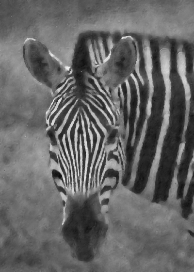
In Fig. 10 a natural image with additive white Gaussian noise ( $N\sim\mathcal{N}(0,0.2)$ , $PSNR=14dB$ ) is denoised. Filtering is performed using OrthoNS, based on the $p$ -Laplacian with $p=1.01$ . Modes with high eigenvalues (lower extinction time) are filtered out. This yields an edge preserving denoising. As expected, we lose some small details but the zebra’s texture in general is preserved.

4.3.3 Spectrum

In Fig. 11 we demonstrate a qualitative comparison between the nonlinear spectral $p$ -decomposition of [25], the OrthoNS decomposition and the posterior OrthoNS. We apply these methods on the zebra (Fig. 10a) for $p=1.01$ . On the left column, the spectra of the $p$ -decomposition, the OrthoNS, and the posterior scheme are given. The images from the second left column to the right represent four different bands in the spectra. One can see that the bands are automatically sorted from fine to coarse spatial structures.

4.4 Run time Vs. Image size

A prominent advantage of this method is the running time. The $p$ -decomposition [25] requires evaluating the (p-Flow) with a uniform small step size. Then, fractional derivative is calculated pointwise. This involves applying FFT and IFFT (along the sampling time axis) for every point in the image. In Fig. 12, we show the computation time versus the size of the image.

Figure 12: Running time Vs. Image size

The $X$ -axis indicates the size of the image (number of pixels) in log scale and the $Y$ -axis indicates the running time taken to compute the decomposition. The running time of OrthoNS is considerably lower than [25] in 1-2 orders of magnitude.

5 Conclusion and future work

In this work we investigated how to recover the main modes of homogeneous gradient flows through a linear dimensionality reduction algorithm. We examined DMD, a leading method for this purpose in fluid-dynamics. We used explicit analytic solutions of such flows for cases where the initial condition is an eigenfunction of the nonlinear operator. The analytic solution of DMD in these cases clearly shows its inability to express such flows faithfully. A significant observation is that DMD can recover well homogeneous flows which are of degree one. We thus proposed a time re-scaling of the sampling points, such that it mimics the dynamics of 1-homogeneous flows sampled with uniform time steps. It was shown how this adaptation allows to fully recover the dynamics with analytic solutions.

Following these insights, two algorithms were proposed for time re-scaling, also when the original time samples and the operator of the flow are not known. Additionally, a different DMD optimization was suggested in order to obtain a symmetric DMD matrix (for non-oscillating flows). We have shown that the modes correspond to approximations of nonlinear eigenfunctions (with respect to the operator of the flow). The OrhoNS mode decomposition was proposed. It yields a small set of the main modes of the flow and can be viewed as a linearization of the nonlinear spectral decomposition ( $p$ -spectra) introduced in [25]. We believe this analysis and proposed representation can further advance the understanding of gradient flows and be used in various fields, wherever such flows are relevant.

List of Symbols

$P$	A nonlinear homogeneous operator
$f$	An initial condition
$\lambda$	An eigenvalue of $P$
$a(t)$	A decay profile
$F(\psi,f)$	A fidelity term
$R(\psi)$	A regularization term
$\partial_{p}siR$	The variational derivative of $R$
$T_{ext}$	The extinction time. The smallest time for which the system gets its steady state
$\nabla$	The gradient of a function
$J_{p}$	The Dirichlet energy
$\Delta_{p}$	The $p$ -Laplacian operator
$dt,\,dt_{k}$	A fixed step size, a step size from $k-1$ th sample to the $k$ th
$f$	Belongs to $\mathbb{R}^{M}$ (column vector), the initial condition of the dynamical system
$\psi_{k}$	The snapshot of the system after $k$ th step in $\mathbb{R}^{M}$ (resulted from sampling or evolving a explicit scheme)
$\Psi_{0}^{N-1},\Psi_{1}^{N}$	Data matrices $[\psi_{0},\cdots,\psi_{N-1}],[\psi_{1},\cdots,\psi_{N}]$
$U,\Sigma,V$	SVD (SVD) of $\Psi_{0}^{N-1}$
$U_{r},V_{r}$	Sub-matrices of $U,V$ containing the first $r$ columns
$\Sigma_{r}$	Sub-matrix of $\Sigma$ containing the most significant $r$ eigenvalues of the SVD which are the diagonal of $\Sigma$
$X,Y$	Dimensional reduced matrices of $\Psi_{0}^{N-1},\Psi_{1}^{N}$ , respectively
$F$	The DMD matrix ,approximating a linear mapping from $X$ to $Y$ (size $r\times r$ )
$w_{i}$	A column vector, the $i$ th right eigenvectors of $F$
$W$	$W=[{\bm{w_{1}}},\cdots,{\bm{w_{r}}}]$
$\{\phi_{i},\mu_{i},\alpha_{i}\}_{i=1}^{r}$	Modes, eigenvalues, and coefficients resulted form DMD (DMD)
$D$	$D=diag([\mu_{1},\cdots,\mu_{r}])$
${\bm{\tilde{\psi}_{k}}}$	Data reconstruction by DMD (discrete time setting)
$A$	$M\times M$ matrix, approximating a linear mapping from $\Psi_{0}^{N-1}$ to $\Psi_{1}^{N}$
${\bm{\tilde{\psi(t)}}}$	Data reconstruction by DMD (continuous time setting)
$ERR_{DMD}$ , $ERR_{Rec}^{d}$ , $ERR_{Rec}^{c}$	The DMD, the (time-discrete) and the (time-continuous) reconstruction errors
$\{\tilde{\mu}\}_{i=1}^{r}$	Eigenvalues in the time continuous setting
$\tilde{dt}_{k},\,\tilde{t}_{k}$	Rescaled step size and time point
$\lambda_{\phi},\,\lambda_{\mu}$	A nonlinear eigenvalue restoration via the mode $\phi$ , the eigenvalue $\mu$

Appendix A Finding a symmetric DMD matrix

We are looking for linear mapping, $F$ , between $X$ and $Y$ when the mapping is symmetric, i.e.

\min_{F}\norm{Y-FX}^{2}_{F},\hskip 9.24994pts.t.\,\,F=F^{T}.

(45)

In addition, according to the spectral theorem every symmetric real matrix can be diagonalized. Therefore, we can express the matrix as $F=Q^{T}DQ$ when $Q$ and $D$ are orthogonal and diagonal matrices. We can rewrite this expression as $F=Q^{T}\sqrt{D}^{T}\sqrt{D}Q$ . Then, we can reformulate the optimization problem as

\min_{F}\norm{Y-FX}^{2}_{F},\hskip 9.24994pts.t.\,\,F=B^{T}B.

(46)

Note, that $B$ is over the complex field and ^T denotes for the transpose operator. Embedding the constrain in the optimization expression, we get

\min_{B}\norm{Y-B^TBX}^{2}_{F}.

Using $\norm{Y-B^TBX}^{2}_{F}=\Tr{Y-B^TBX}^{T}\{Y-B^{T}BX\}$ and the derivatives

\begin{split}\frac{\partial}{\partial B}\Tr{FBG}&=F^{T}G^{T}\\ \frac{\partial}{\partial B}\Tr{FB^TG}&=GF,\end{split}

we get that the minimizer, $B$ , admits

B^{T}BXX^{T}+XX^{T}B^{T}B=XY^{T}+YX^{T}.

Substituting $B^{T}B$ with $F$ , we get that for the minimizer, $F$ , of (45) the following Sylvester equation holds

FXX^{T}+XX^{T}F=XY^{T}+YX^{T}.

(47)

The solution for $F$ exists and unique in this case. There are plenty of algorithm to solve this equation (see e.g. [52][53][54]). In addition, for the specific form of the Sylvester equation (47) a farther study was conducted in [55][56][57]. We use the Matlab implementation (command “sylvester”) for solving the Sylvester equation, which is based on the algorithm of Hessenberg-Schur method. The implementation is based on the routines SB04QD.

Appendix B SDMD (SDMD)

(a)

\lambda=-0.5

(b)

\lambda=0.7

Figure 13: Spectrum Reconstruction. We compare DMD [13], tlsDMD [39], fbDMD [41] and SDMD based on their approximation for the eigenvalue of system (48) when various levels of noise are introduced,

-4\leq SNR\leq 4

Here, we implement the SDMD on a discrete stable linear system

\psi_{k+1}=\begin{bmatrix}0.1&0.6\\ 0.6&0.1\end{bmatrix}\psi_{k}.

(48)

The eigenvalues are $\lambda_{1,2}=-0.5,0.7$ and the initial condition is a normalized summation of the eigenvectors (namely $[1,0]^{T}$ ). We approximate the eigenvalues of this system based on $8$ snapshots in presence of white Gaussian noise. We repeat our experiment $N=1000$ times and average of each of the methods. In Fig. 13 we showcase the results and plot the ellipses which enclose the region of $95\%$ of the estimates that are closest to the true eigenvalue for each of the techniques (see [41]). One can see that for this kind of systems, DMD is superior on the tlsDMD and the fbDMD. In particularly, a method that takes into account the system and its inverse is doom to fail for every stable system since the inverse system is not stable. Therefore, whilst the fbDMD has good performances when the roots are on the unit cycle (BIBO stability) it fails when the roots are in the unit cycle.

Appendix C Proof of Theorem 3

Proof.

The functional $R(\psi)$ is convex, therefore

R(\psi)-R(0)\leq-\langle P(\psi),\psi-0\rangle.

The functional $R$ is zero at the point $0$ (it is assumed to be in its kernel). And thus

R(\psi)\leq-\langle P(\psi),\psi\rangle.

Applying the Brezis chain rule [58], we can write

\begin{split}\frac{d}{dt}R(\psi)=\langle-P(\psi),\psi_{t}\rangle=\langle-P(\psi),-\frac{\langle P(\psi),\psi\rangle}{\norm{P(\psi)}^{2}}P(\psi)\rangle=\langle P(\psi),\psi\rangle\leq-R(\psi).\end{split}

Using the Grönwall’s inequality, we can write $R(\psi(t))\leq R(\psi(0))\cdot e^{-t}=R(f)\cdot e^{-t}$ . Therefore, it converges.

Let the initial condition, $f$ , be an eigenfunction of $P$ with a corresponding eigenvalue $\lambda\neq 0$ ( $f$ is not trivial). Then, the initial condition is an eigenfunction of the operator $G$ with the corresponding eigenvalue $-1$

G(f)=-\frac{\langle P(f),f\rangle}{\norm{P(f)}^{2}}P(f)=-\frac{\lambda}{\lambda^{2}}\frac{\langle f,f\rangle}{\norm{f}^{2}}\lambda f=-f.

In addition, the operator $G(\cdot)$ from Eq. (TRC) is a one-homogeneous operator. Then, the solution is [25] $\psi(t)=f\cdot e^{-t}$ .

∎

References

[1] Norman Ricker. Wavelet contraction, wavelet expansion, and the control of seismic resolution. Geophysics, 18(4):769–792, 1953.
[2] Michael Elad and Michal Aharon. Image denoising via learned dictionaries and sparse representation. In 2006 IEEE Computer Society Conference on Computer Vision and Pattern Recognition (CVPR’06), volume 1, pages 895–900. IEEE, 2006.
[3] Shamgar Gurevich, Ronny Hadani, and Nir Sochen. The finite harmonic oscillator and its applications to sequences, communication, and radar. IEEE Transactions on Information Theory, 54(9):4239–4253, 2008.
[4] Mihailo R Jovanović, Peter J Schmid, and Joseph W Nichols. Sparsity-promoting dynamic mode decomposition. Physics of Fluids, 26(2):024103, 2014.
[5] Yuya Ohmichi. Preconditioned dynamic mode decomposition and mode selection algorithms for large datasets using incremental proper orthogonal decomposition. AIP Advances, 7(7):075318, 2017.
[6] Vardan Papyan, Yaniv Romano, Jeremias Sulam, and Michael Elad. Theoretical foundations of deep learning via sparse representations: A multilayer sparse model and its connection to convolutional neural networks. IEEE Signal Processing Magazine, 35(4):72–89, 2018.
[7] Andrew Y Ng, Michael I Jordan, and Yair Weiss. On spectral clustering: Analysis and an algorithm. In Advances in neural information processing systems, pages 849–856, 2002.
[8] Damian Kaliroff and Guy Gilboa. Self-supervised unconstrained illumination invariant representation. arXiv preprint arXiv:1911.12641, 2019.
[9] Uri Shaham, Kelly Stanton, Henry Li, Boaz Nadler, Ronen Basri, and Yuval Kluger. Spectralnet: Spectral clustering using deep neural networks. arXiv preprint arXiv:1801.01587, 2018.
[10] Tamar Rott Shaham, Tali Dekel, and Tomer Michaeli. Singan: Learning a generative model from a single natural image. In Proceedings of the IEEE International Conference on Computer Vision, pages 4570–4580, 2019.
[11] Martin Burger, Guy Gilboa, Michael Moeller, Lina Eckardt, and Daniel Cremers. Spectral decompositions using one-homogeneous functionals. SIAM Journal on Imaging Sciences, 9(3):1374–1408, 2016.
[12] Shai Biton, Nadav Arbel, Gilad Drozdov, Guy Gilboa, and Amir Rosenthal. Optoacoustic model-based inversion using anisotropic adaptive total-variation regularization. Photoacoustics, 16:100142, 2019.
[13] Peter J Schmid. Dynamic mode decomposition of numerical and experimental data. Journal of fluid mechanics, 656:5–28, 2010.
[14] Da Kuang, P Jeffrey Brantingham, and Andrea L Bertozzi. Crime topic modeling. Crime Science, 6(1):12, 2017.
[15] Naman Agarwal, Brian Bullins, Elad Hazan, Sham Kakade, and Karan Singh. Online control with adversarial disturbances. In International Conference on Machine Learning, pages 111–119, 2019.
[16] Léon Bottou, Frank E Curtis, and Jorge Nocedal. Optimization methods for large-scale machine learning. Siam Review, 60(2):223–311, 2018.
[17] Stanley Osher, Bao Wang, Penghang Yin, Xiyang Luo, Farzin Barekat, Minh Pham, and Alex Lin. Laplacian smoothing gradient descent. arXiv preprint arXiv:1806.06317, 2018.
[18] Paula Gradu, John Hallman, and Elad Hazan. Non-stochastic control with bandit feedback. arXiv preprint arXiv:2008.05523, 2020.
[19] Sanjeev Arora, Elad Hazan, Holden Lee, Karan Singh, Cyril Zhang, and Yi Zhang. Towards provable control for unknown linear dynamical systems, 2018.
[20] Travis Askham and J Nathan Kutz. Variable projection methods for an optimized dynamic mode decomposition. SIAM Journal on Applied Dynamical Systems, 17(1):380–416, 2018.
[21] Romain Leroux and Laurent Cordier. Dynamic mode decomposition for non-uniformly sampled data. Experiments in Fluids, 57(5):94, 2016.
[22] Florimond Guéniat, Lionel Mathelin, and Luc R Pastur. A dynamic mode decomposition approach for large and arbitrarily sampled systems. Physics of Fluids, 27(2):025113, 2015.
[23] Bernard O Koopman. Hamiltonian systems and transformation in hilbert space. Proceedings of the national academy of sciences of the united states of america, 17(5):315, 1931.
[24] Igor Mezić. Spectral properties of dynamical systems, model reduction and decompositions. Nonlinear Dynamics, 41(1-3):309–325, 2005.
[25] Ido Cohen and Guy Gilboa. Introducing the p-laplacian spectra. Signal Processing, 167, 2020.
[26] Ido Cohen, Adi Falik, and Guy Gilboa. Stable explicit p-laplacian flows based on nonlinear eigenvalue analysis. In International Conference on Scale Space and Variational Methods in Computer Vision, pages 315–327. Springer, 2019.
[27] Guy Gilboa. A spectral approach to total variation. In International Conference on Scale Space and Variational Methods in Computer Vision, pages 36–47. Springer, 2013.
[28] Guy Gilboa. A total variation spectral framework for scale and texture analysis. SIAM journal on Imaging Sciences, 7(4):1937–1961, 2014.
[29] Leon Bungert, Martin Burger, Antonin Chambolle, and Matteo Novaga. Nonlinear spectral decompositions by gradient flows of one-homogeneous functionals. arXiv preprint arXiv:1901.06979, 2019.
[30] Oren Katzir. On the scale-space of filters and their applications. Master’s thesis, Technion — Israel Institute of Technology, Haifa 3200003, March 2017.
[31] Guy Gilboa. Nonlinear Eigenproblems in Image Processing and Computer Vision. Springer, 2018.
[32] Andrei Nikolaevich Tikhonov, AV Goncharsky, VV Stepanov, and Anatoly G Yagola. Numerical methods for the solution of ill-posed problems, volume 328. Springer Science & Business Media, 2013.
[33] Leonid I Rudin, Stanley Osher, and Emad Fatemi. Nonlinear total variation based noise removal algorithms. Physica D: nonlinear phenomena, 60(1-4):259–268, 1992.
[34] Arjan Kuijper. p-laplacian driven image processing. In 2007 IEEE International Conference on Image Processing, volume 5, pages V–257. IEEE, 2007.
[35] Martin Welk and Joachim Weickert. PDE evolutions for M-smoothers in one, two, and three dimensions. Journal of Mathematical Imaging and Vision, pages 1–29, 2020.
[36] Gilbert Strang. Linear algebra and learning from data. Wellesley-Cambridge Press, 2019.
[37] Lloyd N Trefethen and David Bau III. Numerical linear algebra, volume 50. Siam, 1997.
[38] J Nathan Kutz, Steven L Brunton, Bingni W Brunton, and Joshua L Proctor. Dynamic mode decomposition: data-driven modeling of complex systems. SIAM, 2016.
[39] Maziar S Hemati, Clarence W Rowley, Eric A Deem, and Louis N Cattafesta. De-biasing the dynamic mode decomposition for applied koopman spectral analysis of noisy datasets. Theoretical and Computational Fluid Dynamics, 31(4):349–368, 2017.
[40] Shervin Bagheri. Effects of small noise on the dmd/koopman spectrum. Bulletin Am. Phys. Soc, 58(18):H35, 2013.
[41] Scott TM Dawson, Maziar S Hemati, Matthew O Williams, and Clarence W Rowley. Characterizing and correcting for the effect of sensor noise in the dynamic mode decomposition. Experiments in Fluids, 57(3):42, 2016.
[42] Omri Azencot, Wotao Yin, and Andrea Bertozzi. Consistent dynamic mode decomposition. SIAM Journal on Applied Dynamical Systems, 18(3):1565–1585, 2019.
[43] Taku Nonomura, Hisaichi Shibata, and Ryoji Takaki. Dynamic mode decomposition using a kalman filter for parameter estimation. AIP Advances, 8(10):105106, 2018.
[44] Taku Nonomura, Hisaichi Shibata, and Ryoji Takaki. Extended-kalman-filter-based dynamic mode decomposition for simultaneous system identification and denoising. PloS one, 14(2), 2019.
[45] Matthew O Williams, Ioannis G Kevrekidis, and Clarence W Rowley. A data–driven approximation of the koopman operator: Extending dynamic mode decomposition. Journal of Nonlinear Science, 25(6):1307–1346, 2015.
[46] Qianxiao Li, Felix Dietrich, Erik M Bollt, and Ioannis G Kevrekidis. Extended dynamic mode decomposition with dictionary learning: A data-driven adaptive spectral decomposition of the koopman operator. Chaos: An Interdisciplinary Journal of Nonlinear Science, 27(10):103111, 2017.
[47] Omri Azencot, N Benjamin Erichson, Vanessa Lin, and Michael W Mahoney. Forecasting sequential data using consistent koopman autoencoders. arXiv preprint arXiv:2003.02236, 2020.
[48] Ido Cohen and Guy Gilboa. Energy dissipating flows for solving nonlinear eigenpair problems. Journal of Computational Physics, 375:1138–1158, 2018.
[49] Joachim Weickert. Anisotropic diffusion in image processing, volume 1. Teubner Stuttgart, 1998.
[50] Jürgen Appell, Espedito De Pascale, and Alfonso Vignoli. Nonlinear spectral theory, volume 10. Walter de Gruyter, 2008.
[51] Matan Gavish and David L Donoho. The optimal hard threshold for singular values is $4/\sqrt{3}$ . IEEE Transactions on Information Theory, 60(8):5040–5053, 2014.
[52] Antony Jameson. Solution of the equation ax+xb=c by inversion of an m*m or n*n matrix. SIAM Journal on Applied Mathematics, 16(5):1020–1023, 1968.
[53] Lu Tongxing. Solution of the matrix equation ax- xb= c. Computing, 37(4):351–355, 1986.
[54] Richard H. Bartels and George W Stewart. Solution of the matrix equation ax+ xb= c [f4]. Communications of the ACM, 15(9):820–826, 1972.
[55] Salle La and S Lefschet. Stability by lyapunov’s direct method. Academic Press, New York, 1961.
[56] RA Smith. Matrix calculations for liapunov quadratic forms. Journal of Differential Equations, 2(2):208–217, 1966.
[57] S Barnett and C Storey. Analysis and synthesis of stability matrices. Journal of Differential Equations, 3(3):414–422, 1967.
[58] Haim Brezis. Opérateurs maximaux monotones et semi-groupes de contractions dans les espaces de Hilbert, volume 5. Elsevier, 1973.