Probabilistic Inversions for Time–Distance Helioseismology
Abstract
Time–distance helioseismology is a set of powerful tools to study localized features below the Sun’s surface. Inverse methods are needed to robustly interpret time–distance measurements, with many examples in the literature. However, techniques that utilize a more statistical approach to inferences, and that are broadly used in the astronomical community, are less-commonly found in helioseismology. This article aims to introduce a potentially powerful inversion scheme based on Bayesian probability theory and Monte Carlo sampling that is suitable for local helioseismology. We first describe the probabilistic method and how it is conceptually different from standard inversions used in local helioseismology. Several example calculations are carried out to compare and contrast the setup of the problems and the results that are obtained. The examples focus on two important phenomena that are currently outstanding issues in helioseismology: meridional circulation and supergranulation. Numerical models are used to compute synthetic observations, providing the added benefit of knowing the solution against which the results can be tested. For demonstration purposes, the problems are formulated in two and three dimensions, using both ray- and Born-theoretical approaches. The results seem to indicate that the probabilistic inversions not only find a better solution with much more realistic estimation of the uncertainties, but they also provide a broader view of the range of solutions possible for any given model, making the interpretation of the inversion more quantitative in nature. The probabilistic inversions are also easy to set up for a broad range of problems, and they can take advantage of software that is publicly available. Unlike the progress being made in fundamental measurement schemes in local helioseismology that image the far side of the Sun, or have detected signatures of global Rossby waves, among many others, inversions of those measurements have had significantly less success. Such statistical methods may help overcome some of these barriers to move the field forward.
Keywords:
Helioseismology, Inverse Modeling; Interior, Convective Zone; Oscillations, SolarI Introduction
Inversions play a critical role for the interpretation of helioseismic measurements. In global helioseismology, inversions of the frequency spectrum of the Sun’s low-degree modes have been used to determine its interior structure (Christensen-Dalsgaard et al. 1996), including internal differential rotation (Thompson et al. 2003; Howe 2009). In the local framework of seismology, inversions of wave-packet travel times, or of ring parameters, are employed for measuring sub-surface flows (Komm et al. 2007), such as meridional circulation (Giles et al. 1997; Zhao et al. 2013; Jackiewicz et al. 2015; Rajaguru & Antia 2015), supergranulation (Zhao & Kosovichev 2003; Švanda 2012), and velocity structures in the vicinity of sunspots (Couvidat et al. 2006; Gizon et al. 2009; Moradi et al. 2010).
Helioseismic inversions estimate sub-surface quantities. Two popular classes of techniques used for this estimation are Regularized Least Squares (RLS) and Optimally Localized Averages (OLA) (Gough & Thompson 1991; Christensen-Dalsgaard et al. 1993; Pijpers & Thompson 1994; Schou et al. 1994; Corbard et al. 1997; Jensen et al. 1998; Jackiewicz et al. 2008; Švanda et al. 2011; Jackiewicz et al. 2012; Korda & Švanda 2019). These methods rely on inversions of large matrices that may suffer from numerical instabilities when the matrices are ill-conditioned, which they often are. Furthermore, the cost or misfit function to be minimized may be very irregular in the parameter space, and strong regularization or smoothing often needs to be applied. Due to various tuning strategies, it is recognized that computing these inversions is sometimes as much “art” as science (Basu 2016).
An alternative framework to interpret observational data relies on Bayesian theory and statistics. In its simplest form, Bayesian inference combines prior information on a model and its parameters with observational data to produce a posterior probability distribution function (PDF hereafter) of the model parameters. The PDF represents the complete solution to the inverse problem, and all of the information is formulated in terms of probabilities. For this to work, one must know the statistical properties of the noise in the data. For helioseismology, these properties are typically well understood (Gizon & Birch 2004; Fournier et al. 2014).
The Bayesian computation of the PDF spans the whole model space. In the case that the PDF is Gaussian, then the inverse problem can be straightforwardly solved using the methods described above to give a reasonable “most-probable model.” However, if the nature of the data or prior information is complex, such that the PDF is not very smooth or is multimodal, then a most-probable model has little meaning. In this case, it is important to characterize the full shape of the PDF as to provide realistic uncertainties on the estimations. The problem becomes one of sampling, rather than optimization.
This is where methods of Markov Chain Monte Carlo (MCMC hereafter) come in. Modern MCMC techniques are actively being developed that efficiently and effectively sample multi-modal, multi-dimensional distribution functions of the parameter space. They work by drawing random samples that are distributed according to the properties of the PDF. Coupling these samplers to Bayesian inferences to solve problems is what will be referred to in this article as probabilistic inversions.
Apart from Earth seismology, which has a very mature MCMC inversion literature (Sambridge & Mosegaard 2002, see the references within, and the references to), global helioseismology and asteroseismology have employed probabilistic methods much more sparsely. The applications have not primarily been for standard inversions either, but for statistical measurements of the properties of individual seismic mode parameters (frequencies, amplitudes, linewidths) (Corsaro & De Ridder 2014, e.g. the Diamonds package of). Local helioseismology has seen even less adoption. A notable exception is the current solar coronal seismology work led by I. Arregui (see Arregui 2018, and references therein). In other areas of astronomy, probabilistic inversions have proven to be a robust way to interpret astronomical observations (Sharma 2017). Indeed, in a relatively recent article presenting a new MCMC Bayesian tool for the Python programming language, Foreman-Mackey et al. 2013 discuss its usage for general astronomical problems. That publication has over 3000 citations in ADS (as of January 2020). A couple dozen are related to asteroseismology, but none to local helioseismology.
Therefore, we feel it could be useful to provide some examples of probabilistic inversions for local helioseismology. This article is written for people working in the field of solar physics and helioseismology who might not be very familiar with the utility of such techniques. We caution that there will be few details in the derivation of Bayesian statistics and MCMC, so that more focus can be appled to example tools and methods that can be used to solve certain classes of helioseismic problems.
The rest of the article is organized as follows: In Section II, the basic formulations of standard linear inversions and Bayesian inferences are described, as well as how they are connected in certain cases. Section III provides examples of both types of inversions for two relevant problems in local helioseismology: inferring the flows of meridional circulation and those of supergranulation. This section compares in detail the results and outputs from the inversions. The final sections present a discussion of when one inversion technique might be preferable to another, and we end with a summary of the work presented. The appendices provide more details of the inversions, as well as a brief description of the probabilistic inversions in a simplified example to understand their usefulness at a conceptual level.
II Deterministic and Bayesian Inferences
II.1 Formulation of Standard Helioseismic Inversions
The majority of local helioseismic inversions published over the last decade or so rely on variants of the Optimally Localized Averages (OLA) method that was developed for terrestrial seismology by Backus & Gilbert 1968. The most widely used form of this class of linear, deterministic inversions may be the Subtractive OLA (Pijpers & Thompson 1994; Jackiewicz et al. 2008; Švanda et al. 2011; Jackiewicz et al. 2012; Greer et al. 2016, SOLA: ). However, some recent studies have begun to employ full-waveform techniques that are very promising, yet very computationally demanding. The methods are iterative in nature and do not assume linearity between the response of seismic waves and the perturbation. Hanasoge and collaborators are at the forefront of this effort (Hanasoge et al. 2011; Hanasoge 2014; Bhattacharya & Hanasoge 2016), which also has a mature history in terrestrial seismology.
In any case, SOLA inversions essentially provide a way to infer the perturbation one spatial location at a time. Unlike RLS-type algorithms, which try to find a best fit to the data, SOLA forms linear combinations of the data (while minimizing the errors) that spatially localize the inference. The solution can critically depend on the tuning of certain parameters. These are not model parameters, but parameters that control the type of solution one desires. There are tradeoffs in the solution, such as those between spatial resolution and noise amplification, which are tunable. There are also parameters that allow for regularizing of possible ill-conditioned, large matrices. The choices of these parameters can be somewhat subjective and non-rigorous.
Standard derivations of the SOLA method are common in the literature (Švanda et al. 2011; Jackiewicz et al. 2012; Korda & Švanda 2019, e.g.). Here, a slightly modified version is presented that will connect to the probabilistic equations in Section II.2. We follow closely the notation of Tarantola 2005. Where appropriate, the relationship to standard inversion terminology is given in parenthesis with italicized text.
Assume any model can be described by , where denotes space. By model, we mean the quantity that inversions are seeking, such as the flow structure of a supergranule or the sound-speed profile under sunspots. Consider a generalized discrete dataset that is linearly related to the model through an integral equation
| (1) |
where is some functional that describes the physics of the problem. If such an equation exists, it will be called a generative model. For now, this relationship will be given as
| (2) |
where vector functions (sensitivity kernels). The true, but as of yet unknown, model is related to some set of observed data through
| (3) |
which we consider error free for simplicity. We want to obtain a good estimate of at some location, and we therefore assume that the estimator model is linearly related to the observed data as
| (4) |
where the are constants (weights). Defining some resolution operator (averaging kernels) as
| (5) |
gives
| (6) |
This equation implies that the estimation that will be found is a smoothed version of the true model, since with finite data will never be a delta function.
The constants [] are computed by minimizing a cost function
| (7) |
where represents a delta function, but in practice it is something more reasonable (Gaussian target function). Minimization with respect to the weights gives
| (8) |
This expression shows that a (usually) large matrix inversion is necessary to compute (kernel convolution matrix).
Finally, once the weights are obtained, the estimate is given by
| (9) |
and
| (10) |
Notice that the observations are only involved in the last step: the calculation of is not conditioned on the data at all.
It is interesting to point out that the model estimate is likely not the true model (again using a finite amount of data). So it is reasonable to postulate that the true model may have a form in which it is related to the estimated model, plus some arbitrary, properly scaled model of similar smoothness
| (11) |
This expression serves as a general solution to the inverse problem
II.2 Background to Bayesian inferences
Full discussions of MCMC in the general context of Bayesian theory and astronomy applications can be found in many places (Sharma 2017; Hilbe et al. 2017, e.g.). A particularly useful pedagogical treatment is given by Hogg & Foreman-Mackey 2018. Here a simple overview is provided to guide the later discussion and examples.
Imagine we have measurements of some observable comprising a data set , and each measurement has an uncertainty , which are normally distributed . Now assume that we possess a generative model that can, in principle, make predictions of the data through the operation , as in Equation 1. is a model made up of parameters . If many repeated measurements are made, then the expected frequency distribution (probability) of datum is
| (12) |
The vertical bar is read as “given,” so this expression is the probability of the datum given the model and the uncertainty on . Clearly, if the operation
| (13) |
gives a number far from , the resulting probability will be small. One wishes to maximize the probability, not just of one data point, but the entire set of observations. This is usually referred to as the likelihood function , which is a product of individual probabilities
| (14) |
In practice, one may stop here and find the parameters that maximize the likelihood function, or, more conveniently, minimize the negative logarithm of it. The problem then reduces to least-squares fitting. The resulting model, identified from the probability of the data given the parameters, is interpreted, however, as the likelihood of the parameters given the data. This interpretation presents a formal inconsistency.
Bayes’s Theorem can be easily derived from sum and product rules of probability theory. The result has four quantities. One quantity is the likelihood function in Equation 14. Another is any prior information [] that we possess on the model and the uncertainties, which will be denoted . The third is the evidence, [], which is a effectively a normalization term and will not be important for our discussion. The final ingredient is the posterior probability distribution function, which is computed as
| (15) |
and defines Bayes’s Theorem. This important quantity is the statistical probability of the model given the data, uncertainties, and any prior knowledge.
The model PDF is therefore related to the likelihood function, and it will closely resemble it if the priors are not very specific or informative. In this case the interpretation stated above is not so fatal. However, some of the power of the Bayes framework is that if the prior knowledge of model parameters is non-trivial, then the PDF is too, and its complexity requires more sophisticated inference methods to be applied. Priors also restrict the parameter space to a smaller region than a likelihood function alone can.
In general, and in the examples below, the likelihood function is a multivariate normal distribution
| (16) |
where is the data covariance matrix, is its determinant, and is the dimension of the problem (length of ).
To summarize, probabilistic inversions use Equation 15 to compute the posterior PDF – the joint probability distribution of parameters that is consistent with the data. The PDF will rarely have an analytic form, and it is not necessarily well-behaved or uni-modal. The goal is not to optimize (maximize) the PDF, or find its peak, but to know the whole distribution and sufficiently sample it. One can imagine one strategy, which would be looping over a (uniform) grid of parameter values and computing the resulting PDF. However, for high-dimensional problems, this would be extremely expensive and inefficient. Too many low-probability realizations would be calculated. Fortunately, there are alternative approaches. There is a robust literature of different probability distribution sampling methods, but most modern ones rely on MCMC techniques. The basic difference among these methods is how the sampler “moves” through the parameter space; i.e. how an algorithm decides to choose trial parameter values, so that it hopefully spends more time in high-probability space. MCMC uses random numbers to drive the process. Metropolis–Hastings is one of the simplest and well-known algorithms (Press et al. 2007).
A recently developed MCMC algorithm, affine-invariant sampling (Goodman & Weare 2010), is what we adopt in this work. This method is in a class of ensemble MCMC, since multiple chains, called “walkers,” are all in execution simultaneously as they explore the parameter space. The walkers can therefore be run in parallel, but they are allowed to interact in certain ways to adapt the proposal densities and maintain their Markov properties. It is a promising tool for sampling PDFs that are not extremely complex (Foreman-Mackey et al. 2013).
The connection of the SOLA inversion described in Section II.1 to the probabilistic language where priors and covariances are considered is useful, and it can be made quite easily. Consider a linear least-squares problem. Including model priors, one could construct a cost function (or least-squares function, or -function) as
| (17) | |||||
| (18) |
and are the covariance matrices of the data and model priors (if known), respectively. As outlined above, the Gaussian posterior PDF can be computed from the cost function that has a form . The center of the distribution, i.e. the most likely model of the Gaussian PDF (the model that minimizes the cost function) and its covariance can be computed by differentiation and shown to be
| (19) | |||||
| (20) |
In the SOLA method, there are no priors in the model space. In the probabilistic language, this implies white noise with no correlations and a (possibly) infinite variance of the priors:
| (21) |
Using the definitions in Section II.1, the posterior centers then reduce to
| (22) | |||||
| (23) |
The first equation is precisely Equation 11, a general solution of a SOLA inversion with the prior information replacing the arbitrary model . In the SOLA language, if (a -function like averaging kernel), then . In the probabilistic language, this implies there are no uncertainties in the posterior solution, so .
These two conclusions are identical, showing that, in principle, the methods can arrive at similar results, yet only in ideal circumstances. What is hopefully demonstrated throughout the rest of this article is that the probabilistic method, in practice, is robust, practical, and gives more uncertainties.
III Examples for Time–Distance Local Helioseismology
The forward problem in time–distance helioseismology is symbolically formulated as (Kosovichev & Duvall 1997; Gizon & Birch 2002; Gizon & Birch 2004, e.g.)
| (24) |
where the travel-time shifts [] between two surface locations are caused by some (small) interior perturbation . The sensitivity kernels [] mediate this relationship, which is considered to be linear. Any inversion consists of using the observed surface and computed to find the unknown . In SOLA methods, is inferred at each spatial location, or at least one depth at a time. In probabilistic inversions, must first be parametrized by some number of free parameters. The parameters are estimated using Bayes’s theorem and MCMC, and then can be studied over the whole domain.
We elucidate two rather simple examples of inversions based on common research areas in local helioseismology. We compare the probabilistic inversions with the SOLA method and contrast the computational particulars. We will only consider examples of flows, and therefore travel-time differences are the important observables.
It is important to keep in mind that in what follows we are not solving any real problem. In one case, we are only inverting synthetic observations that are computed in the forward sense from Equation 24. This does not tell us anything about the accuracy of the sensitivity kernels. They could be completely wrong. It only tells us about the inverse process, which is the goal here. In the other case, inversions of a realistic numerical model are shown. Most helioseismic studies employ two ways of modeling the interaction of seismic waves with inhomogeneities: ray theory or Born theory. Our examples span these two cases.
III.1 Meridional Circulation in a Ray-Theory Approach
III.1.1 The Toy Problem


We use a simple, single-cell, meridional-flow model first described by van Ballegooijen & Choudhuri 1988 and utilized by Dikpati & Charbonneau 1999, among others. The parametric model is given by Equations 57 – 61 of van Ballegooijen & Choudhuri 1988 and will not be reproduced here. For our purposes, the meridional profile has effectively three free parameters, which will be denoted , , and . controls the flow amplitude, while and control the latitudinal and radial (depth) dependence of the flow structure, respectively. The model provides two-dimensional flows in the radial and latitudinal directions that satisfy mass conservation in the 2D domain: . The input values of the three parameters are such that the poleward surface flow reverses direction at . We use a grid that has 150 points in latitude and 100 points in radius, covering and from to .
Ray kernels are computed for a set of latitudes and distances that sample the model relatively well (although by no means exhaustively). We consider ten skip distances from to . The central latitude range is , resulting in a total of 122 ray kernels. Figure 1 shows the given circulation model with all ray paths overplotted. The weaker radial flows of the model are not shown here.
Synthetic forward travel-time differences are then computed from the flow model and kernels, shown on the right of Figure 1. To these travel times, artificial, random noise is added at two different levels: In the low-noise case, is about 2 % of the rms of the travel-time differences (0.8 seconds), and about 20 % in the high-noise case ( These noise levels roughly correspond to typical measurements made over three years and one month, respectively (Braun & Birch 2009).
III.1.2 SOLA Solution to the Problem


We first demonstrate the standard inversion method described in Section II.1. It is the SOLA inversion applied by Jackiewicz et al. 2015 and other recent studies. The synthetic travel-time differences are considered to be uncorrelated, and thus the noise-covariance matrix used in the inversion is diagonal. No mass-conserving constraint is imposed, and therefore it is hopeless to try to recover the small radial velocity in this inversion, which is about 10 % of the amplitude of the latitudinal flows.
The SOLA inversion estimates the velocities at specific target locations. In this example, there are 110 target locations, 10 in depth and 11 in latitude. At each location, a 2D Gaussian target function was computed with a full-width-half-maximum (FWHM) in the radial direction of and in the latitudinal direction of . The target function replaces the unrealistic function given in Equation 7, and it gives a measure of the spatial resolution of the inversion results.
The results of the SOLA inversion are shown in Figure 2 after inverting the low-noise and the high-noise travel times. To aid in comparison with the known model, the retrieved flows at the 110 spatial locations have been interpolated onto the model grid. The recovered flows generally follow the pattern of the model. The deeper return flow is not reliably found in either case. Since the SOLA inversion always returns a flow pattern that is a smoothed version of the real one (Jackiewicz et al. 2012; Švanda 2012, see), the amplitude is underestimated. On average, the underestimation is about in the low-noise case, about in the high-noise case, but in some locations up to
The inferred noise is too small and not consistent with the errors. Specifically, the retrieved velocity is away from the input in the high-noise case. In other words, if the true answer were not known and we surmised that our result is within 1 or 2 away from the truth, we would make an error of one order of magnitude. Another feature of the inversions reveals the expected less-localized averaging kernel for the case of the noisier travel times. Note that one can tune the trade-off parameters to obtain different results (smoother/less noisy, more localized/noiser, etc.), making the interpretation of the validity of the inferences challenging.
III.1.3 Probabilistic Solution to the Problem: Parameter Posteriors

Before showing the results of the Bayesian MCMC inversion in a standard way, it is important to explore the output at the level of the walkers and the multidimensional PDF of the parameters. In this example, the total number of steps (iterations) was chosen to be . Each of the three free parameters was assigned 60 walkers (chains). The sampling of each walker was every five steps, which is a “thinning” procedure, whereby only the fifth step is stored. The PDF was therefore sampled times per walker. The choice of the standard deviation of Gaussian likelihood function is second. Since the measurements are assumed to be uncorrelated, , the likelihood function in Equation 16 reduces to
| (25) |
The priors are taken as flat and rather wide, for demonstration purposes, as if we did not have a good idea of their values.
Figure 3 shows the time series of all of the walkers during the run. Upon inspection, the first thing to point out is that the initial steps are when the sampling “burns-in.” This essentially means that the chains take a few steps to wander towards and reach a high-probability region, since the starting values typically might be far from such regions, as in this example (by choice). There is endless debate about burn-in validity in the literature (e.g. Hogg & Foreman-Mackey 2018, Section 7) into which we will not delve. In any case, the walker behavior is acceptable, in that once burnt-in, the space of the PDF is fully explored. The acceptance rate of the proposed steps is about 30 % – a good value for MCMC algorithms.
Sample draws can be correlated in MCMC algorithms due to noise or other factors. If each draw were completely independent, then the variance would decrease as more and more samples are drawn. It is critical to know if independent samples are drawn from the PDF so that the parameter estimation is not biased, and reliable estimates of the mean/median and variance can be computed. The standard way of determining this is by calculating the autocorrelation of the walkers of each parameter. When and if the autocorrelation approaches zero, one can be confident that the walkers “lose their memory” of where they started and reach some state of equilibrium. The autocorrelation can be computed empirically from the time series of walkers, and it is shown in Figure 3 in the right panel. In this case, the rate of convergence is quite rapid compared to the length of the run, and even fewer total steps could have been chosen. The effective sample size (ESS) is another concept to understand how many independent samples were drawn in the walker time series, and it is found from the autorcorrelation (Sokal 1997). In this example, the ESS is 1168. For a standard deviation of the PDF of a given parameter, the Monte Carlo standard error goes as . This means that we are able to measure the median of a parameter with about a 3 % error compared to the overall uncertainty .

The PDF in this example is three-dimensional. The “corner” plot matrix in Figure 4 shows histograms of all of the one- and two-dimensional projections of the PDF of the parameters. The marginalized 1D PDFs are along the diagonal, and correlations between parameters are given in the off-diagonal elements (marginalized 2D PDFs). In this case, the PDFs are not multimodal, which can be an indication that the model is parametrized well. This should not be surprising since the input model follows the same parametrization as the forward model.
The power of the projected model parameter PDFs in Figure 4 is that one immediately sees the distribution widths, as well as any correlations between model parameters. In this example, the PDFs bracket the known input value of the parameters within the 16 and 84 percentiles, except parameter , which is just beyond that range. This parameter also has the least Gaussian PDF.
III.1.4 Probabilistic Solution to the Problem: Model Space

The median of the PDFs of the inversion for the three parameters are used to generate a flow circulation profile. This provides a way to visualize the results in the space of the model, similar to what was shown earlier for SOLA. The resulting profiles are very comparable to the input model, so much so that in Figure 5 only the differences with the model are shown. The differences are significantly less than the SOLA example described in Section III.1.2. In the low-noise example, the inversion very slightly overestimate the poleward flow amplitude (parameter ), and therefore the equatorward flow is weakly underestimated. This affects the radial-velocity differences in the manner shown. In the case of noisier travel times, is again overestimated, but the other two parameters are slightly underestimated, leading to some small-scale differences in the relative flows.
III.1.5 Probabilistic Solution to the Problem: Data Space

The MCMC method allows for a visualization of the results in data space too, much more naturally and quickly than the SOLA method. Figure 6 presents the data-space solutions for both inversion methods using noisier travel times. One immediately sees the manifestation of the underestimated velocity in the SOLA inversion in the smaller-amplitude travel times. The near-surface region (left of the figure at smaller skip distances) is particularly evident. On the other hand, the travel times generated from the median of the PDF are highly consistent with the input ones. Also shown are 100 random realizations of the PDF, which quickly gives a picture of the statistical uncertainties in the data space.
III.2 Supergranulation in the Born theory
The Sun’s supergranulation is an important component of near-surface convection-zone dynamics and a strong source of advection of magnetic fields. While its sub-surface flow structure has not yet been faithfully determined by helioseismology, it may have a simple enough form to be parametrized by a model. It is therefore another suitable test case for a probabilistic inversion. For this example, we consider five new aspects that add complexity and richness to the demonstration:
- •
The problem is set up in three dimensions (rather than two);
- •
Born-sensitivity kernels are used (instead of ray kernels);
- •
The observations are from a 3D numerical simulation with stochastic, realistic noise properties (not synthetic forward-modeled observations);
- •
A proper noise covariance matrix is computed and used in the inversions (not just diagonal variances); and
- •
The supergranule model in the simulation is different from the model and parameters used to estimate the PDF.
Regarding the last point, this means that the “true” values of the parameters used to simulate the supergranule are essentially unknown, unlike the meridional-flow example where the input could be directly compared to the posteriors. We briefly describe the problem setup before studying the results.
III.2.1 The Models
The supergranulation model is taken from Dombroski et al. 2013. In that work, realistic wave propagation using the SPARC code (Hanasoge et al. 2006) was simulated through a single, kinematic supergranule flow pattern to quantify the effects on seismic waves. The mass-conserving flow structure was modeled using seven parameters. Two control the horizontal extent of the divergent flow, three control the depth-dependence and strength of the outflow, and two more parameters control the depth dependence of the boundary inflow.
The has a radial extent of about Mm at the surface, where the maximum horizontal speed and the vertical speed is and , respectively. The outflow switches to an inflow at a depth of Mm. The maximum vertical speed is about , peaked around Mm below the photosphere. For purposes later, this will be referred to as the reference (“ref”) model.
As a notable aside, while this model is reasonable and at least consistent with surface observations (Duvall & Birch 2010; Rieutord & Rincon 2010), supergranulation has proven very difficult to fully understand. There are even questions about whether models that have separable flows (in horizontal and vertical directions) are appropriate for supergranulation (Ferret 2019; Dhruv et al. 2019). Addressing such issues is beyond the scope of this article.
The model that we use in the probabilistic inversion is instead from Duvall & Hanasoge 2012. Also employing a separable, mass-conserving flow, this model has five free parameters. In fact, two of the parameters are equivalent between the models, those that control the horizontal diverging flow as
| (26) |
where is an order-one Bessel function, is a wavenumber, and represents a decay length in the distance coordinate from the origin []. The values from Dombroski et al. 2013 are and Mm, identical to those in Duvall & Hanasoge 2012. In addition, this model has a Gaussian depth-dependence of the velocities, determined by three additional parameters: a peak amplitude [], a peak flow location [], and a Gaussian width [], leading to the function
| (27) |
Once is computed, the model vertical flows are constructed first as . Then the horizontal flows are , where is obtained from applying the continuity equation. We compute this model in three spatial Cartesian dimensions for illustration sake, even though it is axisymmetric and the problem can be solved in only two. This will be referred to as the “trial” model.
Apart from the two common free parameters, each model is derived differently enough that the priors on the other three free parameters are not well known. We take uniform priors that are kept identical in each of the probabilistic inversions discussed below. The priors are given in Table 1.
| Parameter | Label | Min. | Max. | Unit |
|---|---|---|---|---|
| 50 | 400 | |||
| 0 | 12 | Mm | ||
| 0 | -12aaNegative values denote sub-surface | Mm | ||
| 20 | 40 | |||
| 10 | 25 | Mm |
III.2.2 Setup of the Problem
Helioseismic measurements were computed from the numerical simulation using a time series of the vertical velocity, which is sampled every 1 minute at 200 km above the model photosphere over a total of 24 hours. The horizontal spatial domain extends 100 Mm and is sampled every 1/3 Mm. The vertical velocity is first filtered to isolate different ridges (radial orders ), including the -mode () and the first two acoustic-mode ridges (, ) using standard methods (Braun & Birch 2008b; Gizon et al. 2009; DeGrave et al. 2014). Cross correlations were measured in center-to-annulus and center-to-quadrant geometries for 15 different travel distances, ranging from 6 Mm to 20 Mm. For each ridge and each distance, three travel-time difference maps are computed (at the same spatial resolution) across 50 Mm of the simulation domain: “out–in” [], “west–east” [], and “north–south” []. Such geometries are sensitive to flows (Duvall et al. 1997). This results in 135 unique travel-time maps, which are very comparable to the ones computed using helioseismic holography by Dombroski et al. 2013. Only a fraction of these measurements are used in the sample inversions.
Dombroski et al. 2013 computed a second simulation without a background supergranule. We use these data (split into twelve two-hour cubes) to estimate the noise covariance in the travel times according to the noise model of Gizon & Birch 2004. The exact same measurement procedure explained above is carried out on these cubes to determine the covariances .
The linear forward problem (Gizon & Birch 2002) in this example can be written
| (28) |
where flows are , the sensitivity kernels are vector-valued, and each index corresponds to a given ridge, geometry, and travel distance. Born-approximation kernels are computed from Birch & Gizon 2007 in a point-to-point fashion, and then averaged over annuli to be consistent with the travel-time geometries . The -superscripts refer to the particular measurement source or supergranule model under consideration.
We can be precise about this example. The SOLA inversion is looking to infer in Equation 28 given the kernels and the measurements of , and so . Let’s call the estimate . The probabilistic inversion is using Equation 28 with and the same kernels to forward compute , thus in that case. The are used in the computation of the likelihood function along with . In model space, the probabilistic inversion is seeking to estimate suitable values of parameters such that will resemble . Further details in the setup of the inversions are mentioned in Appendix A.
III.2.3 Results
SOLA inversions in 3D are not very convenient to compare with the probabilistic inversions, neither in model space nor data space. The reason is that, typically, the flows in are inferred one depth at a time, and these depths are usually few. Furthermore, the prescribed “resolution” in both directions can vary from depth to depth. In this example, the SOLA inversions were carried out at three target depths Mm. Each target depth had a different target width in the horizontal and vertical directions. The actual depth at which the inversion is most sensitive can also be distant from due to non-localized averaging kernels. By contrast, and by construction, the probabilistic inversions provide parameters that allow one to estimate flows over the full (or any) spatial domain.
To make meaningful comparisons between inversion results and the reference model, several steps need to be taken. Since the SOLA results are rather coarse in depth and smooth in the horizontal direction, we decide to adapt everything else to them. Firstly, for a given target depth, the reference model velocities are convolved with the target function of the inversion [the in Equation 7, which in this case is not a -function but a 3D Gaussian sphere]. This process is represented by Equation 6, whereby the estimated flows are a smoothed version of the true ones: . The result is then integrated over depth, giving a 2D flow map that can be compared to the SOLA inferences.


For the probabilistic inversion, we use draws of the model PDF parameters (median or otherwise) and compute the flow model on the same spatial grid as and the . It is also appropriately smoothed by the SOLA inversion target function and integrated over depth in the same manner. This process results in three sets of flow maps at three nominal target depths for three flow components, although we restrict comparisons to and . Only results in model (velocity) space will be presented.
Figure 7 shows a comparison of these two flow components at 3 Mm beneath the photosphere, where the horizontally divergent structure is apparent. In general, we find the SOLA inversions severely underestimate horizontal velocities (note the scaling factor), while the probabilistic inversions weakly overestimate them. The bottom panel of Figure 7 shows a cut through the models at . The noise in the SOLA inversion, even using covariance matrices, is highly underestimated. The horizontal error bars show the FWHM of the target function, which were quite wide to get sensible results. On the other hand, a random sample of the parameter PDF from the probabilistic inversion gives a reasonable spread of solutions in model space.
At the same depth, the inferences on the weaker vertical velocity are also shown in Figure 7 on the right. In this case, the SOLA flow inferences are marginal at best. At inversions just below this depth, the SOLA flows are anticorrelated with the reference flows, as in Figure 11 in Appendix B. Dombroski et al. 2013 found the same result in their inversions of this model, and they demonstrated that the culprit was the “cross talk” between vertical and horizontal flows that the sensitivity kernels, and inversions, are unable to disentangle. In our SOLA inversion, an explicit cross-talk term is included (Švanda et al. 2011), and even still, the problem persists. The sensitivity kernels are not completely accurate. This can be verified by comparing measured and forward-modeled travel-time differences, and as Dombroski et al. 2013 showed (and we verified) there are anomalies in some of the travel-time maps. However, since both inversions use the same kernel functions, the relative comparsions are meaningful. Examples at other depths are given in Appendix B.
Figure 9 in Appendix B shows the corner plot for the probabilistic inversion. The only “known” parameters are and , so comparisons between the input ones and inferred ones cannot be made due to the differing models. The probabilistic inversion overestimates the flow speeds, and is mainly due to the estimation of the and parameters (Section III.2.4 gives more evidence of this). These control the location of the peak of the vertical-velocity profile and its width. There are (at least) two reasons for the poor estimation of and . The first, as the corner plot shows in the 2D marginalized PDFs, is that these two parameters are not highly correlated with the others, but more so with themselves. There must be some correlations due to the continuity-equation constraint, but it is a weak one. This could indicate a poor parametrization of this particular model for supergranulation11 1 Indeed, the conclusions from earlier work using this model (Duvall & Hanasoge 2012; Duvall et al. 2014) showed a very shallow supergranule that is quite different than what other studies have found in the literature. While the analysis may very well be correct, more checks on the model need to be carried out, which is beyond the scope of this article. The second reason has to do with the sensitivity functions used here. They have very little sensitivity below 8 Mm, while the depth of the profile extends to a depth of about 12 Mm. The likelihood is thus not informative, and the 1D PDF for parameter is not very Gaussian.
III.2.4 Does Additional Data Bring New Information?
For researchers who have experience computing inversions in local helioseismology, it can be non-trivial to understand how the addition of extra observations will (positively or adversely) affect the results. Indeed, a brief discussion regarding this point is presented by Dombroski et al. 2013 in their results section. For instance, consider one set of measurements using particular seismic waves. Now, consider another set of measurements using the same seismic waves but where the only difference is different travel distances. Will including the second set with the first improve the inversion, just add unwanted noise, or improve the noise? Just doing this experiment may not answer the question either, since the differences may be subtle, and SOLA or RLS inversions can be very sensitive to measurement points.
The probabilistic inversion provides a way to study this question more quantitatively. We design a simple demonstration experiment, and leave a full analysis to another article. Eleven probabilistic inversions are computed, each one having different combinations or different numbers of input data sets. Everything else is kept fixed.
Two metrics are then calculated to assess the results. We compare the variance of the priors to the variance of the posteriors. Imagine the worst case scenario, when the variance is not reduced at all. This would imply that the addition of data has provided no new information on the model parameters. The goal of any inversion is to reduce the variance of the parameter estimation. The variance reduction metric is computed as
| (29) |
where is the prior distribution function (Equation 15) whose range of values is in Table 1. The other metric is the simple correlation coefficient between the travel-time measurements and the forward measurements computed using the median of the PDF.

The results are provided in Figure 8. To understand what is shown, consider, for example, the second row of the matrix. means there are two travel-time maps used, and for the -mode at a travel distance of 6 Mm. The black for these quantities are filled. To the right of the dashed line, the variance reduction of the five parameters (as a percentage) are given by the gray scale. To be specific, the values for through in row 2 are . The data have not provided much information on at all, as suspected. After that, is the correlation coefficient, and is the slope of a simple linear fit between the travel-time vectors. In almost all trials, the inferred data have larger amplitudes ().
The third row is an inversion with only one change: the measurements are removed and an extra travel distance is added. The precise values of the variance reduction are now . The first parameter has gone from dark gray to black, over the 80 % level, and are marginally worse, and is marginally better. Finally, the fourth row also uses two sets of measurements, with only one annulus geometry and one distance, but now two ridges ( and ). This results in a better variance reduction of than the other cases, and brings the slope closer to one. One might conclude, for this scenario, that given a very limited number of measurements, it is best to use more ridges than adding distances or anything else.
One can continue this way for the other cases to find interesting trends. Inspecting the matrix as a whole, a few things stand out. and are the best “resolved” parameters, and and are the least. A quick glance at the PDFs in the corner plot in Figure 9 confirms this. The last row in the matrix is from an inversion using 18 different travel-time maps, and the variance reduction for and are 62 % and 40 %, respectively, the best in the set. The correlation between maps is consistently high, and the slope fluctuates a bit, but is overall acceptable.
To answer the question posed in this subsection – yes, at least in this particular example. While the addition of new data might not visually and qualitatively improve the comparison in data space or model space (as evidenced by the unchanging correlations), the variance, or uncertainties of the parameters, generally does improve.
In principle, such an analysis could also be achieved from the SOLA inversions, but it would be more cumbersome. Minimizing the cost function properly, i.e. calculating a good averaging kernel, becomes much more difficult with fewer and fewer kernels. Then the trade-off parameters change and some of the results would not be sensible. However, in the probabilistic framework, this is entirely reasonable and instructive.
IV Discussion
The previous sections have contrasted two linear methods for interpreting helioseismic measurements. For comparison, we label the class of inversions similar to SOLA as Method 1, and the class of statistical and probabilistic inverions as Method 2. There are several similarities between these two approaches. Both methods require a type of forward equation relating the unknowns and measurements. Several such equations are provided (Equations 1, 24, 28). Both methods can be run numerically using parallelization when formulated appropriately.
The practical differences outnumber the similarities. Method 2 needs more than a forward equation; it requires a generative model that can be parametrized with a manageable number of parameters. It would be difficult to utilize Method 2 to make synoptic flow maps of the Sun that contain many different convective structures and size scales, as standard “pipeline” inversions now do for local helioseismic data (Zhao et al. 2012). Method 1 does not use the data until the last step, whereby it combines the measurements in an “optimal” way based on how the sensitivity functions were combined . Method 1 requires ways to deal with computing the inverse of a large, usually ill-conditioned matrix. Method 2 provides a statistical interpretation of the solution, while Method 1 is forced to provide a “best model.”
Beyond similarities and differences, inversion methods need to be validated. Numerous helioseismic studies over the past decade have employed numerical models for validation purposes. This is a powerful strategy, since one can quantitatively test inversion results on the known answer from the model. The results of these studies provide very consistent conclusions. On the one hand, there are those that use Method 1 and measurements of (non-magnetic) numerical models that do not have realistic noise, although usually some form of noise is added to the measurements after the fact. The findings are generally encouraging (Hartlep et al. 2013; Jackiewicz et al. 2015; Korda & Švanda 2019, e.g. example 1 in this article;). This would seem to indicate rather persuasively that Method 1, as well as the sensitivity functions (either ray or Born), can be used to accurately solve problems. On the other hand, when more realistic simulation models are studied in the same way, the results are somewhat in agreement near the surface, but quickly diverge below Mm (Zhao et al. 2007; Dombroski et al. 2013; DeGrave et al. 2014; DeGrave et al. 2018, example 2 in this article;). The solar-like realization noise in these models is a significant barrier, which brings skepticism to any inversion results using actual solar data and Method 1 (Braun & Birch 2008a; Švanda 2015; Korda et al. 2019, as commented on by).
Despite heroic efforts and substantial progress, there unfortunately have not been as many significant advancements as one would expect in our understanding of the Sun from explicit inversions of local helioseismic data (Gizon et al. 2010). The two examples in this work are cases in point, where still no consensus has been established (Giles et al. 1997; Zhao et al. 2013; Rajaguru & Antia 2015; Liang & Chou 2015; Jackiewicz et al. 2015; Duvall & Hanasoge 2012; Hathaway 2012; Greer et al. 2016).
Indeed, most of the fundamental breakthroughs in local helioseismology have come from the observations alone, rather than the formal interpretation of them. Examples include far-side imaging from acoustic holography and time distance (Lindsey & Braun 2000; Zhao 2007), direct imaging of large-scale flows (Woodard 2002), acoustic absorption by sunspots (Braun et al. 1987), flared-induced sunquakes (Kosovichev & Zharkova 1998), and the recent detection of solar Rossby waves using different helioseismic measurement strategies (Löptien et al. 2018; Hanasoge & Mandal 2019; Proxauf et al. 2019), among many others.
The potential issues that inhibit a full helioseismic analysis of certain outstanding problems include systematics and realization noise inherent in measurements, the theoretical treatment of seismic wave scattering from solar perturbations, and the inverse methods applied. There are many ways for dealing with each of these factors at various levels, and this work provides a possible avenue forward for exploration of the inversion component.
V Summary and Outlook
In this article we described a probabilistic inversion scheme for time–distance helioseismology that uses Bayesian statistics and Monte Carlo sampling. A few simple examples were carried out and compared with the commonly used SOLA technique. The examples used synthetic data where the known answer was the target of the inversions. Given that the input sets of measurements and sensitivity functions were rather minimal, the goal was not to solve these problems completely (i.e. infer the flows as well as possible), but to demonstrate some of the strengths and weaknesses of these two approaches.
While the examples were highly idealized, the intercomparison consistently showed that the SOLA inversions systematically underestimate the flow speeds and the noise levels, the probabilistic inversions also crucially provide informative posterior probability distribution functions on the model parameters that are more consistent with the known answer. One may question the need to use for (likely) highly linear problems like meridional circulation. In some of the example cases, however, the posteriors are not Gaussian, which could be a possible reason why SOLA or least-squares methods are not optimal. At the very least, the probabilistic method could be used to explore which helioseismic problems have complex PDFs and demonstrate why other inverse methods get trapped in local minima.
SOLA inversions can be tuned at some level to obtain different properties of the solution. A particular advantage of the probabilistic inversion scheme is that many realizations of the solution (in data space and/or model space) are computed automatically, allowing for a broad view of any particular model and its relative probability given the data.
Future work in this area should concentrate on developing well-parametrized models of solar structures amenable to helioseismic investigation. For example, the recent meridional circulation model of Liang et al. 2018 is much more flexible than the one presented here. Good models may also increase computational efficiency. Finally, one could imagine forward (generative) models that compute other observables than travel times, such as the more fundamental and information-laden cross correlations. This would be another move in the direction of full-waveform inversions.
While this work is focused on time–distance helioseismology, application to ring-diagram analysis, helioseismic holography, or direct modeling is straightforward. For those interested in similar applications, the affine-invariant ensemble MCMC algorithm has been made available in Python (emcee: https://github.com/dfm/emcee) and Matlab (GWMCMC: https://github.com/grinsted/gwmcmc) and can be adapted to many types of problems.
Appendix A Supergranulation Inversion Details

This article presents a comparison of six SOLA inversions (two flow components at three target depths) to the probabilistic one for a simulated supergranule model. For completeness, details of the inversions and how they are compared are itemized here:
- •
The simulation domain is Mm on a side horizontally, sampled evenly at Mm. It extends to Mm at the bottom boundary. Cross correlations and travel times were measured in an area Mm on a side at the same sampling. Each map is therefore points.
- •
Born sensitivity kernels are computed on the same horizontal grid as the travel times and they extend to 15 Mm below the surface using 55 points in depth. The kernels use input model power spectra that have been Fourier filtered to separately retain the first 3 radial orders, including the -mode. Everything is computed to match the details of the travel times as discussed in Section III.2.2.
- •
The SOLA inversion code is the faster formulation in Fourier space that can be run in parallel (Jackiewicz et al. 2012). It includes a cross-talk parameter as in Švanda et al. 2011. Trade-off curves (L-curves) were studied to find the best regularization parameters. To obtain sensible results in terms of noise and misfit, the 3D Gaussian target functions have FWHM on the order of 10 Mm and 3 Mm in the horizontal and vertical directions, respectively. In general, the SOLA inversion results are very similar to the ones published by Dombroski et al. 2013 using an RLS inversion scheme.
- •
The probabilistic inversion has steps. Each of the five parameters was assigned 120 walkers. With thinning every five steps, the PDF was sampled times per walker, as before. More walkers were used in this inversion than the meridional example because the PDFs are more complicated, and it is suggested to use more walkers for good sampling. These values are sufficient to give good autocorrelation properties of the walker time series.
- •
The data vector is composed of only a small subset (12 of the 135) of the travel-time measurement maps. To speed up the computation, each of the pixel maps was binned down to only pixels. The data vector is therefore 4332 measurements. To match the size of the data vector, the forward vector resulting from the operation uses kernels that are also binned down. This is noteworthy, in that the SOLA inversion uses the full maps. The probabilistic inversion is quite powerful with substantially less data. Of course, the 4332 measurements are not all completely independent, as described by the covariance matrix.
- •
The full noise covariance matrix used in the likelihood function (Equation 16) was constructed from smaller pairs of covariances and ordered to correctly match the travel-time data vector.
- •
The uniform priors on the model are given in Table 1. As is common (Foreman-Mackey et al. 2013), the walkers are initialized with values in a small Gaussian ball, centered somewhere within the prior bounds. The initial guess is not critical, as the walkers soon quickly explore the full parameter space after the burn-in stage.
- •
The entire run on a two-core desktop machine (thus minimal parallelization) was about 80 minutes. The most expensive task is the computation of the forward travel times in Equation 28, which takes about 0.2 seconds each.
Appendix B Supergranulation Flow Inversions
A few more results are presented here to add to those in Section III.2.3. The corner plot for the probabilistic inversion is given in Figure 9.
The flow inversion comparison near the top of the simulation domain is shown in Figure 10. For the horizontal flows, the SOLA inversion underestimates the (smoothed) flow amplitude by about a factor of two, while the probabilistic inversion overestimates the amplitude by . The profile structure is primarily determined by parameters and . The peak vertical velocity is underestimated by 35 % in the SOLA inversion, and it is overestimated by 60 % in the probabilistic inversion. The -mode is generally the most sensitive at these layers, but its sensitivity to vertical flows is weak. This affects both inversions. also has artifacts in its flow structure.
A comparison near 5 Mm beneath the surface is given in Figure 11. As is common in standard helioseismic inversions using typical data sets, the inferences at this depth are uninformative (Zhao et al. 2007). The vertical velocity inferred is weak and is the wrong sign, which was also noticed in Dombroski et al. 2013. The probabilistic inversion provides a good estimate of the flow structure at this depth.


Appendix C Why do probabilistic inversions work better?
The comparisons of the different inversion methods reveal that the probabilistic ones are more robust at inferring the true flows in the examples provided. To try to understand these results at a conceptual level, it is necessary to look at simpler examples that remove unneccesary complications.
We will focus on a problem that is basic, yet very similar to the form of helioseismic inversions – recovering an image that has been blurred and corrupted with noise. Consider an initial image and the operation
| (C1) |
where is some blurring operator and is independent Gaussian noise with zero mean []. is the resulting image that represents the “data.” This expression closely resembles the relationship between travel-time measurements and (), sensitivity kernels (), internal flows (), and the inherent noise in travel times ().
To make this even more straightforward, we will take to be a binary image of a curly W letter, which only has values of (black) and (white). An example of and the resulting data () with signal-to-noise ratio (SNR) of is shown in Figure 12. The goal is to use the corrupted image on the right to try to infer the original image on the left.

C.1 SOLA-Type Solution
One of the most straightforward ways of solving this image-recovery problem that most closely relates to the SOLA formulation described in the article is using a least-squares estimate. In fact, it is almost completely analogous to SOLA mathematically. The problem of estimating requires solving
| (C2) |
The least-squares solution can be found analytically as
| (C3) |
where is the covariance matrix, which in this case is diagonal with value . Note the similarity to Equations 7 and 9.
The solution computed using Equation C3 is shown in Figure 13 in the left panel. Evidently, the solution is very unstable, as the matrix A is ill-conditioned and sparse with small values, which causes the inverse (if it exists, as it does in this case) to blow up. There are methods to avoid this behavior by regularizing the problem. Instead of solving Equation C2, one rewrites the problem as
| (C4) |
where solutions can be controlled by a regularization parameter . The analytic solution in this case is
| (C5) |
where is the identity matrix, and the covariance matrix has been omitted for clarity. The regularizing parameter essentially controls the smoothness of the reconstructed image. When small, the solution fits the data well at the expense of amplified noise and not being smooth; when large, the solution is smooth but does not fit the data well. The key is that the solution either resembles in some fashion but is very noisy, or is smoother with a much smaller amplitude.
This is demonstrated in Figure 13 in the final three panels, which are computed using Equation C5. When there is minor regularization, the image shows the curly W, but with rather high-amplitude pixels caused by the noise amplification. The maximum values reach about 20, and the rms over all pixels is 4 (the rms of the original image is 1). Even though this solution is technically the best fit to the data, it is very noisy. As is common in helioseismic inversions, an “L”-curve can be computed from the series of solutions based on the regularization trade off. The optimal regularization solution in the third panel is where the bend in the “L”-curve occurs in this example. It represents a compromise between smoothness and noise. The final panel is overly regularized and smooth, with the letter almost completely washed out. Its values are between .
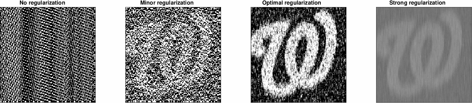
In this example, as in SOLA inversions for helioseismology, a set of solutions is calculated based on different levels of regularization. The “best” solution is not chosen arbitrarily, but it is chosen with little guidance about the physics of the problem. It is the solution that “looks good,” and is mostly due to the addition of an unphysical regularization parameter. If none of the solutions look good, there are not many options left.
C.2 Probabilistic Solution
The image reconstruction inverse problem can also be solved in a probabilistic fashion using the Bayesian formalism. One strategy is to try to determine, for every pixel in the noisy image, if it came from a in or from a in the original.
First, we need a likelihood function and priors. The likelihood function of the data () given some model image estimate () of the true image is
| (C6) |
where the sum is over all x pixels in the image. The value of any th pixel in our model can only take on or .
The Bayesian framework allows one to use various priors. A uniform prior means that any model image is equally probable, and each pixel is independent from every other pixel. In this case, uniform priors do not work so well. The reason is that for noisy images made up with pixels of large amplitude, the probability that any pixel was derived from is very similar to the probability it came from . From testing, this does not help significantly reduce the noise on the reconstructed image.
However, using a priori knowledge that the goal is to reconstruct the binary image of a letter, where pixels of the same value tend to be clumped together, we can compute a more useful prior in the following fashion. A pixel is compared to its four neighbors. If this pixel is embedded near pixels of the same sign, the probability that it has that sign is larger than otherwise. Therefore, the prior for any given pixel can be expressed as
| (C7) |
where is simply the number of neighboring pixels around that have a different sign. is a (positive) tunable coupling constant. A large , for example, produces big blobs of white or black pixels. In these examples we use , which tends to give reasonable results. This prior is motivated by the Ising model used in the study of magnetism in solid-state physics (Brush 1967) and now utilized in many areas of MCMC sampling (Donner & Opper 2017, e.g.). The Ising prior would be, to our knowledge, challenging or impossible to implement in the least-squares inversion framework.
The posterior probability function can now be computed and sampled using MCMC. A few details of how the Markov chains proceed are worthwhile to explain. The model trial image is initialized to all ones. The algorithm iterates pixel-by-pixel. For each pixel, the sign gets flipped as a proposal, and the probability of accepting this new state of the pixel is computed as the ratio of the PDF of the new state to the PDF of the original state. If the ratio is greater than 1, the new state is accepted. If not, a random number is drawn between 0 and 1, and if the number is less the ratio, the new state is accepted anyway. This is a familiar MCMC update procedure (e.g. Metropolis-Hastings), even simpler than the one used in the rest of this article.
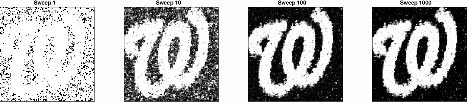
Figure 14 shows a few stages, or sweeps, of the Bayesian inversion as it samples the PDF. A snapshot of the current MCMC state is taken every 10,000 iterations, and the th sweep is an average over snapshots. It is analagous to studying means or other modes of the PDF, rather than the value of a parameter at any state (e.g., the value of any walker at some arbitrary iteration is not very informative). During the first sweep, the model image is initialized to all ones, and after 10,000 proposed pixel flips, the curly W is only marginally visible. Each pixel may only have been visited on average once, or less (). At sweep 10 the algorithm has gone through iterations, and the reconstruction is getting smoother. After iterations, the final recovered image is quite similar to the original one.
C.3 Summary
The Bayesian framework is more flexible and works better than least-squares algorithms for problems of the form of Equation C1, whose form is the generally the same as in helioseismology. Not only do the probablistic inversions work better, they allow for potentially many different types of solutions since they explore the full posterior probability, whose landscape may be complex. The least-square solution only gives one class of solutions, which are often very sensitive to numerical instabilities and noise. With different prior assumptions, other sets of solutions can be explored with the Bayesian method.
C.4 Animations
A few animations of the inversions as they proceed can be found at http://astronomy.nmsu.edu/jasonj/MCMC/. The three animations show example reconstructions using both methods for different noise levels ; for , , and . The last case only has an SNR. The animation updates after each sweep of 100,000 iterations. The top panels are the original image and the blurred and noisy image. The bottom left is the current MCMC state, which is a binary image. The bottom center is the image at the th sweep. The bottom right shows the least-squares solution for the given regularization (smoothing), whos value increases with time. All panels have a grayscale with limits set to .
The example with no added noise is interesting. The image is blurred only. The least-squares solution can recover the blurred image, but not the source image, as the Bayesian inversion does.
References
- Arregui (2018) Arregui, I. 2018, Advances in Space Research, 61, 655
- Backus & Gilbert (1968) Backus, G., & Gilbert, J. 1968, Geophys. J. Roy. Astr. Soc., 16, 169
- Basu (2016) Basu, S. 2016, Living Reviews in Solar Physics, 13, 2
- Bhattacharya & Hanasoge (2016) Bhattacharya, J., & Hanasoge, S. M. 2016, ApJ, 826, 105
- Birch & Gizon (2007) Birch, A. C., & Gizon, L. 2007, Astronomische Nachrichten, 328, 228
- Böning et al. (2017) Böning, V. G. A., Roth, M., Jackiewicz, J., & Kholikov, S. 2017, ApJ, 838, 53
- Braun & Birch (2008a) Braun, D. C., & Birch, A. C. 2008a, ApJ, 689, L161
- Braun & Birch (2008b) —. 2008b, Sol. Phys., 251, 267
- Braun & Birch (2009) Braun, D. C., & Birch, A. C. 2009, in Astronomical Society of the Pacific Conference Series, Vol. 416, Solar-Stellar Dynamos as Revealed by Helio- and Asteroseismology: GONG 2008/SOHO 21, ed. M. Dikpati, T. Arentoft, I. González Hernández, C. Lindsey, & F. Hill, 131
- Braun et al. (1987) Braun, D. C., Duvall, T. L., J., & Labonte, B. J. 1987, ApJ, 319, L27
- Brush (1967) Brush, S. G. 1967, Reviews of Modern Physics, 39, 883
- Christensen-Dalsgaard et al. (1993) Christensen-Dalsgaard, J., Hansen, P. C., & Thompson, M. J. 1993, MNRAS, 264, 541
- Christensen-Dalsgaard et al. (1996) Christensen-Dalsgaard, J., Dappen, W., Ajukov, S. V., et al. 1996, Science, 272, 1286
- Corbard et al. (1997) Corbard, T., Berthomieu, G., Morel, P., et al. 1997, A&A, 324, 298
- Corsaro & De Ridder (2014) Corsaro, E., & De Ridder, J. 2014, A&A, 571, A71
- Couvidat et al. (2006) Couvidat, S., Birch, A. C., & Kosovichev, A. G. 2006, ApJ, 640, 516
- DeGrave et al. (2018) DeGrave, K., Braun, D. C., Birch, A. C., Crouch, A. D., & Javornik, B. 2018, ApJ, 863, 34
- DeGrave et al. (2014) DeGrave, K., Jackiewicz, J., & Rempel, M. 2014, ApJ, 788, 127
- Dhruv et al. (2019) Dhruv, V., Bhattacharya, J., & Hanasoge, S. M. 2019, ApJ, 883, 136
- Dikpati & Charbonneau (1999) Dikpati, M., & Charbonneau, P. 1999, ApJ, 518, 508
- Dombroski et al. (2013) Dombroski, D. E., Birch, A. C., Braun, D. C., & Hanasoge, S. M. 2013, Sol. Phys., 282, 361
- Donner & Opper (2017) Donner, C., & Opper, M. 2017, Phys. Rev. E, 96, 062104
- Duvall & Hanasoge (2012) Duvall, T. L., & Hanasoge, S. M. 2012, Sol. Phys., 136
- Duvall et al. (2014) Duvall, T. L., Hanasoge, S. M., & Chakraborty, S. 2014, Sol. Phys., 289, 3421
- Duvall & Birch (2010) Duvall, Jr., T. L., & Birch, A. C. 2010, ApJ, 725, L47
- Duvall et al. (1997) Duvall, Jr., T. L., Kosovichev, A. G., Scherrer, P. H., et al. 1997, Sol. Phys., 170, 63
- Ferret (2019) Ferret, R. Z. 2019, A&A, 623, A98
- Foreman-Mackey et al. (2013) Foreman-Mackey, D., Hogg, D. W., Lang, D., & Goodman, J. 2013, PASP, 125, 306
- Fournier et al. (2014) Fournier, D., Gizon, L., Hohage, T., & Birch, A. C. 2014, A&A, 567, A137
- Giles et al. (1997) Giles, P. M., Duvall, T. L., Scherrer, P. H., & Bogart, R. S. 1997, Nature, 390, 52
- Gizon & Birch (2002) Gizon, L., & Birch, A. C. 2002, ApJ, 571, 966
- Gizon & Birch (2004) —. 2004, ApJ, 614, 472
- Gizon et al. (2010) Gizon, L., Birch, A. C., & Spruit, H. C. 2010, ARA&A, 48, 289
- Gizon et al. (2009) Gizon, L., Schunker, H., Baldner, C. S., et al. 2009, Space Science Rev., 144, 249
- Goodman & Weare (2010) Goodman, J., & Weare, J. 2010, Communications in Applied Mathematics and Computational Science, Vol. 5, No. 1, p. 65-80, 2010, 5, 65
- Gough & Thompson (1991) Gough, D. O., & Thompson, M. J. 1991, The inversion problem, ed. Cox, A. N., Livingston, W. C., & Matthews, M. S., 519–561
- Greer et al. (2016) Greer, B. J., Hindman, B. W., & Toomre, J. 2016, ApJ, 824, 128
- Hanasoge & Mandal (2019) Hanasoge, S., & Mandal, K. 2019, arXiv e-prints, arXiv:1901.06479
- Hanasoge (2014) Hanasoge, S. M. 2014, ApJ, 797, 23
- Hanasoge et al. (2011) Hanasoge, S. M., Birch, A., Gizon, L., & Tromp, J. 2011, ApJ, 738, 100
- Hanasoge et al. (2006) Hanasoge, S. M., Larsen, R. M., Duvall, Jr., T. L., et al. 2006, ApJ, 648, 1268
- Hartlep et al. (2013) Hartlep, T., Zhao, J., Kosovichev, A. G., & Mansour, N. N. 2013, ApJ, 762, 132
- Hathaway (2012) Hathaway, D. H. 2012, ApJ, 749, L13
- Hilbe et al. (2017) Hilbe, J. M., de Souza, R. S., & Ishida, E. E. O. 2017, Bayesian Models for Astrophysical Data Using R, JAGS, Python, and Stan, doi:10.1017/CBO9781316459515
- Hogg & Foreman-Mackey (2018) Hogg, D. W., & Foreman-Mackey, D. 2018, ApJS, 236, 11
- Howe (2009) Howe, R. 2009, Living Reviews in Solar Physics, 6, 1
- Jackiewicz et al. (2012) Jackiewicz, J., Birch, A. C., Gizon, L., et al. 2012, Sol. Phys., 276, 19
- Jackiewicz et al. (2008) Jackiewicz, J., Gizon, L., & Birch, A. C. 2008, Sol. Phys., 251, 381
- Jackiewicz et al. (2015) Jackiewicz, J., Serebryanskiy, A., & Kholikov, S. 2015, ApJ, 805, 133
- Jensen et al. (1998) Jensen, J. M., Jacobsen, B. H., & Christensen–Dalsgaard, J. 1998, in SP, Vol. 418, Structure and Dynamics of the Interior of the Sun and Sun-like Stars, ed. S. Korzennik, 635
- Komm et al. (2007) Komm, R., Howe, R., Hill, F., et al. 2007, ApJ, 667, 571
- Korda & Švanda (2019) Korda, D., & Švanda, M. 2019, A&A, 622, A163
- Korda et al. (2019) Korda, D., Švanda, M., & Zhao, J. 2019, A&A, 629, A55
- Kosovichev & Duvall (1997) Kosovichev, A. G., & Duvall, Jr., T. L. 1997, in ASSL 225: SCORe’96: Solar Convection and Oscillations and their Relationship, ed. F. P. Pijpers, J. Christensen-Dalsgaard, & C. S. Rosenthal, 241–260
- Kosovichev & Zharkova (1998) Kosovichev, A. G., & Zharkova, V. V. 1998, Nature, 393, 317
- Liang & Chou (2015) Liang, Z.-C., & Chou, D.-Y. 2015, ApJ, 805, 165
- Liang et al. (2018) Liang, Z.-C., Gizon, L., Birch, A. C., Duvall, T. L., & Rajaguru, S. P. 2018, A&A, 619, A99
- Lindsey & Braun (2000) Lindsey, C., & Braun, D. C. 2000, Sol. Phys., 192, 261
- Löptien et al. (2018) Löptien, B., Gizon, L., Birch, A. C., et al. 2018, Nature Astronomy, 2, 568
- Moradi et al. (2010) Moradi, H., Baldner, C., Birch, A. C., et al. 2010, Sol. Phys., 171
- Pijpers & Thompson (1994) Pijpers, F. P., & Thompson, M. J. 1994, A&A, 281, 231
- Press et al. (2007) Press, W. H., Teukolsky, S. A., Vetterling, W. T., & Flannery, B. P. 2007, Numerical Recipes 3rd Edition: The Art of Scientific Computing, 3rd edn. (USA: Cambridge University Press)
- Proxauf et al. (2019) Proxauf, B., Gizon, L., Löptien, B., et al. 2019, arXiv e-prints, arXiv:1912.02056
- Rajaguru & Antia (2015) Rajaguru, S. P., & Antia, H. M. 2015, ApJ, 813, 114
- Rieutord & Rincon (2010) Rieutord, M., & Rincon, F. 2010, Living Reviews in Solar Physics, 7, 2
- Sambridge & Mosegaard (2002) Sambridge, M., & Mosegaard, K. 2002, Reviews of Geophysics, 40, 1009
- Schou et al. (1994) Schou, J., Christensen-Dalsgaard, J., & Thompson, M. J. 1994, ApJ, 433, 389
- Sharma (2017) Sharma, S. 2017, ARA&A, 55, 213
- Sokal (1997) Sokal, A. 1997, Monte Carlo Methods in Statistical Mechanics: Foundations and New Algorithms, ed. C. DeWitt-Morette, P. Cartier, & A. Folacci (Boston, MA: Springer US), 131–192
- Tarantola (2005) Tarantola, A. 2005, Inverse problem theory and methods for model parameter estimation (Society for Industrial and Applied Mathematics)
- Thompson et al. (2003) Thompson, M. J., Christensen-Dalsgaard, J., Miesch, M. S., & Toomre, J. 2003, ARA&A, 41, 599
- Švanda (2012) Švanda, M. 2012, ApJ, 759, L29
- Švanda et al. (2011) Švanda, M., Gizon, L., Hanasoge, S. M., & Ustyugov, S. D. 2011, A&A, 530, A148
- van Ballegooijen & Choudhuri (1988) van Ballegooijen, A. A., & Choudhuri, A. R. 1988, ApJ, 333, 965
- Švanda (2015) Švanda, M. 2015, A&A, 575, A122
- Woodard (2002) Woodard, M. F. 2002, ApJ, 565, 634
- Zhao (2007) Zhao, J. 2007, ApJ, 664, L139
- Zhao et al. (2013) Zhao, J., Bogart, R. S., Kosovichev, A. G., Duvall, Jr., T. L., & Hartlep, T. 2013, ApJ, 774, L29
- Zhao et al. (2007) Zhao, J., Georgobiani, D., Kosovichev, A. G., et al. 2007, ApJ, 659, 848
- Zhao & Kosovichev (2003) Zhao, J., & Kosovichev, A. G. 2003, in ESA Special Publication, Vol. 517, GONG+ 2002. Local and Global Helioseismology: the Present and Future, ed. H. Sawaya-Lacoste, 417–420
- Zhao et al. (2012) Zhao, J., Couvidat, S., Bogart, R. S., et al. 2012, Sol. Phys., 275, 375