Pricing service maintenance contracts using predictive analytics
Abstract
As more manufacturers shift their focus from selling products to end solutions, full-service maintenance contracts gain traction in the business world. These contracts cover all maintenance related costs during a predetermined horizon in exchange for a fixed service fee and relieve customers from uncertain maintenance costs. To guarantee profitability, the service fees should at least cover the expected costs during the contract horizon. As these expected costs may depend on several machine-dependent characteristics, e.g. operational environment, the service fees should also be differentiated based on these characteristics. If not, customers that are less prone to high maintenance costs will not buy into or renege on the contract. The latter can lead to adverse selection and leave the service provider with a maintenance-heavy portfolio, which may be detrimental to the profitability of the service contracts. We contribute to the literature with a data-driven tariff plan based on the calibration of predictive models that take into account the different machine profiles. This conveys to the service provider which machine profiles should be attracted at which price. We demonstrate the advantage of a differentiated tariff plan and show how it better protects against adverse selection.
Keywords: maintenance, servitization, contract pricing, predictive analytics, risk management, calibration
1 Introduction
Product maintenance plays a central role in the business model of several manufacturing firms as they change their focus from selling products to selling product-service bundles. In the latter case, firms are responsible for the maintenance and functionality of their products. This servitization trend is motivated by the need to escape the product commoditization trap [Visnjic and Van Looy, 2013]. Service providers and OEMs in the capital goods industry offer a range of service contracts to suit the needs of their customers. Maintenance can either be provided by on-call service, which means that each preventive or corrective intervention is charged to the equipment user based on materials used and time spent. Alternatively, maintenance can be offered under a service plan such as a full-service contract. A full-service contract covers all future costs of preventive and corrective maintenance, over a predetermined time horizon in exchange for a (series of) fee(s) or fixed premium(s). Potentially, these contracts also include down-time compensation, to protect against the moral hazard of being served later than on-call customers. In practice, a company could offer a combination of an on-call and a full-service contract. This hybrid contract could for example only cover periodic maintenance or only certain failure types. Examples of companies shifting their focus on services are General Electric Co., Siemens AG, and Hewlett-Packard Co. [Sawhney et al., 2003].
In this paper, we study full-service contracts from the viewpoint of the service provider, who offers (sells) the contract to the user of the equipment. Under a full-service contract, the user no longer bears the risk of stochastic maintenance costs in exchange for the certitude of a fixed service fee; shifting the risk to the service provider. For the service provider, these contracts offer a guaranteed revenue stream. They are also profitable in case the total premium volume of a portfolio, i.e. the collection of machines covered by a full-service contract, exceeds the maintenance costs.
Accurate price setting is a major challenge for service providers offering full-service maintenance contracts. Simply pricing full-service contracts based on historical estimation of expected total costs incurred over the contract period plus a safety margin (e.g. a factor reflecting the risk-averseness of the service provider times the standard deviation of the historical total costs) does not take the heterogeneity between machines and customers into account. On the one hand, estimating expected costs for only a subset of machines with equal characteristics (by subdividing the data into different classes), stratifies the data into small sample sets for which costs cannot be accurately estimated [Denuit et al., 2007]. As a consequence, a justified price differentiation for a specific customer or machine is less straightforward. On the other hand, if all customers pay the same price for a contract, this may lead to adverse selection. ‘Low-risk’ customers, who require less maintenance and thus should be offered a lower price than maintenance-heavy customers, may not sign a full-service contract when they pay the same premium as the high-risk customers. As a result proportionally more high-risk customers will remain in the portfolio. This phenomenon is also observed in insurance and is detrimental for the profitability of a service contracts portfolio. Market research on services suggests that coming up with profitable service solutions is hard [Gebauer et al., 2005; Hancock et al., 2005; Ulaga and Reinartz, 2011]; it seems that inadequate pricing makes it hard to exploit the financial potential of extended services [Rapaccini, 2015].
In an era of big data and data analytics the collection and statistical analysis of data can provide useful insights to many decision support systems, including tariff plans of full service contracts. We propose a method to determine the price, or premium, of full-service contracts inspired by insights and techniques developed in the actuarial literature. A full-service maintenance contract can be considered an insurance covering the maintenance costs during a certain period of time. A key concept in insurance pricing that can be carried over to pricing full-service maintenance contracts, is the frequency-severity approach of handling claims or incurred costs [Henckaerts et al., 2018; Verbelen et al., 2018, see e.g.]. This involves modelling and predicting the frequency of failures and their associated costs, i.e. severity, separately and (statistically) independent. A second element of insurance pricing is the use of ‘risk factors’ to reflect the heterogeneity of the risks in the portfolio [Henckaerts et al., 2018]. To avoid lapses in a competitive market, insurance companies use rating factors (e.g. age, postal code area) to classify risks and to differentiate prices of their insurance products. Pricing through risk classification is the mechanism for insurance companies to compete as it allows an insurer to express which risk profiles should be attracted at which price. Insurance companies therefore maintain large databases with policy(holder) characteristics, i.e. contract and customer information, and claim histories to build personalized risk-based pricing models.
Using predictive analytics we develop an approach similar to insurance analytics that takes into account risk factors to predict the machine-specific costs under a full-service contract, and price it accordingly. For example, the reliability of a machine can be influenced by operating conditions, operator skills, service history and quality, among others. Some risk factors, such as temperature or humidity, can have a direct influence on the reliability. Other risk factors are proxies for the real influencing factor. For instance, the machine location can be a proxy for the environmental conditions. This information can be collected either by sensors installed on the machines, e.g. temperature measurements, or by sales people or technicians, at the time of sales or at a maintenance intervention respectively. The latter is known as the Internet of people (IoP) and the former as the Internet of things (IoT).
This idea is new in the context of pricing maintenance contracts and will be used to detect which risk factors indicate significant differences in the expected number of maintenance interventions (frequency) and the expected costs incurred (severity). Including these risk factors allows a machine and customer specific tariff plan based on proper risk assessment. A differentiated tariff plan taking the heterogeneity of the machine portfolio into account also provides a better protection against adverse selection and makes the offering of the service provider more competitive.
Our predictive data-driven approach relies on the availability of historical data. We will demonstrate our methodology on simulated data. The use of a simulation data provides a controlled environment to study the performance of our methodology in different scenarios prior to applying it to real data. We develop a simulation engine that is capable to simulate both (time-to-)failure data, and repair and maintenance costs in a variety of different machine environments such that it captures the heterogeneity in the contract data induced by the risk factors. The resulting data format is similar to what can be available to a service provider with a maintenance contract portfolio. The latter has been verified with an industrial partner. We apply our predictive analytics models to our simulated data to determine the break-even price, which is the minimum premium required to have a profitable contract portfolio and we show the economic value of this pricing approach.
2 Literature
The literature on service maintenance contracts makes a distinction between resource-based service and performance-based contracts. With resource-based service, maintenance is priced based on the time and materials spent; it can either be on-call or by use of a full-service maintenance plan. With on-call service the customer contacts the service provider in case of failure and is charged for the corresponding maintenance. In contrast to full-service plans, the customer bears all the maintenance risk. We focus in this article on resource-based full-service contracts. Performance-based contracts ensure the availability (or up-time) of the equipment, and their compensation is based on the availability of the underlying product [Kim et al., 2017]. The literature comparing resource-based and performance-based contracts indicates that product reliability is generally higher under performance-based contracts [Guajardo et al., 2012; Bakshi et al., 2015]. Chan et al., 2018 study sales and service records of medical equipment. Their dataset consists of service records for 700 devices over a four-year period including the maintenance visits and their associated part costs and labor. They analyze the frequency of maintenance visits using a Poisson regression model and their associated part and labor costs using an exponential regression model. They find that moving from on-call service to full-service plans reduces reliability and increases maintenance costs. Not only do operators reduce the level of their own care of the equipment under full-service contracts, the service provider also expends more resources to the equipment.
Rapaccini, 2015 presents a general overview of the literature on pricing service contracts. He distinguishes three pricing approaches: the price can be based on the predicted costs under the contract; it can be based on the perceived value of the service contract; or it can be benchmarked against the price of similar contracts offered by competitors. Our method is a cost-based pricing approach, based on the expected costs of maintenance and repair, which can then be augmented by a desired risk and profit margin. The stochastic and machine-dependent nature of the frequency and severity of failures makes this a non-obvious exercise. When this pricing scheme is then benchmarked with competition, small adaptations can be made for specific machine profiles to ensure that the ‘desired’ profiles are attracted to the portfolio.
Huber and Spinler, 2012; Huber and Spinler, 2014 describe a value-based pricing approach for full-service repair contracts, which do not include preventive maintenance. They first develop a cost-based price, based on the failures and their associated costs, which are modelled independently by a non-homogeneous Poisson process and a distribution with finite support. The value-based price is then obtained by the customer’s choice (and utility) of on-call versus full-service, by means of a mean-variance utility function. Huber and Spinler, 2014 come up with a competition-based price by considering competition with other service providers. Whereas Huber and Spinler, 2012 set out a stochastic model for the frequency of failures and associated costs to price full-service repair contracts, they do not calibrate their model on (historical) maintenance data, neither do they assess the future costs in a contract by a predictive model.
The non-renewing free replacement warranty policy, where the manufacturer repairs or replaces a product at no cost, is similar to full-service contracts. It also involves an upfront payment of the warranty price, which is included in the sales price. Luo and Wu, 2018a; Luo and Wu, 2018b optimize the warranty policy for different product types jointly, by determining the optimal warranty price and the optimal length of the warranty period. The frequency of the incoming warranty claims and their associated costs are modelled as statistically independent. Although the latter is similar to actuarial pricing and the work by Huber and Spinler, 2012; Huber and Spinler, 2014, Luo and Wu, 2018a; Luo and Wu, 2018b do not include product characteristics (as risk factors) in their analysis, nor do they provide a data-driven approach to optimize the warranty policy.
The asset covered by a full-service maintenance contract is a repairable system. The reliability literature discusses how to model time-to-failure for these repairable systems taking into account the effect of both preventive and corrective maintenance actions. We refer to Lindqvist et al., 2006, Wu and Zuo, 2010 and Doyen and Gaudoin, 2011 for an introduction to these models. We use their approach to model the frequency of failures for full-service maintenance contracts.
Motivated by the current state-of-the art in insurance pricing [see Denuit et al., 2007; De Jong et al., 2008, for an overview], our paper extends the literature on service contracts by introducing a data-driven pricing methodology to accommodate price differentiation based on a proper risk assessment using predictive analytics. This is also in line with Luo and Wu, 2018b’s call for data-driven methodologies for warranty contracts and Bertsimas and Kallus, 2020’s insights on the inclusion of covariate data in problems in operations research and management science.
3 Predictive analytics for full-service contracts
In this section we describe the different aspects of a full-service maintenance contract, introduce its break-even price, and propose our methodology to calibrate this price using predictive models. Appendix A gives an overview of the key notations used in the paper.
3.1 Problem description
We consider a service provider who provides maintenance to a collection of machines, potentially of different type, under a full-service contract. We denote this collection of full-service contracts as the contract portfolio. A full-service contract covers all maintenance and repair costs for that machine during a period , with the finite and predetermined duration of the contract. The start of the contract can either be the moment of the machine sale or a later moment. The start can be different for the different machines in the portfolio. During this coverage period , preventive maintenance interventions are included in the contract, which are typically also scheduled at initiation of the contract. Whereas is usually deterministic, the associated costs of preventive maintenance, for , are not. We will assume that each preventive maintenance is of the same type and has the same effectiveness. This does not mean that all preventive maintenances have exactly the same cost – we assume they are intrinsically stochastic, but this difference in costs is not related to the effectiveness; as a result in our model the cost of the preventive maintenance does not impact the subsequent failure intensity. We note that the influence of preventive maintenance actions could be further incorporated via time-varying covariates in our statistical models. These time-varying covariates could represent e.g. the time since last maintenance event, the number of maintenance events in the past year, the cost of the last preventive maintenance, etc.
The contract additionally covers the costs of the corrective maintenance due to unplanned failures and/or due to malfunctioning of a component of the machine that requires repair or even replacement. These can be minor failures, requiring minimal corrective maintenance, or catastrophic failures requiring a major overhaul of the machine. Both the corrective maintenance and the overhaul are unplanned and consequently their occurrence and timing are stochastic. We distinguish between different types of failures, and denote the number of failures of type that occur during the contract period and the associated cost of the th failure of type . Both and are unknown at initiation of the contract.
Figure 1 illustrates the timeline of a contract during the coverage period , with on the horizontal axis (indicating the time dimension) the planned preventive maintenance interventions and the unplanned failures of type , . The vertical lines, for every event, represent the size of the associated costs, and respectively. The probability density functions on the vertical axis illustrate the stochastic nature of these costs.
The total costs covered by the service contract, , equal the total aggregated failure costs and the total aggregated preventive maintenance costs, , covered by the contract over the period :
| (1) |
with
| (2) |
and
| (3) |
We consider the occurrence of a failure and its associated cost to be statistically independent, in line with most literature [Huber and Spinler, 2012; Luo and Wu, 2018a; Luo and Wu, 2018b; Henckaerts et al., 2018]. Taking the dependence between frequency and severity into account is much more involved. This has for instance been done by Gschlößl and Czado, 2007 and Czado et al., 2012. The assumption of independence between severity and frequency of failures is typical in insurance pricing and makes the frequency and severity analysis more tractable.
The preventive maintenance scheme influences the occurrence of failures and consequently affects the failure costs . We consider this maintenance scheme exogenous [Poppe et al., 2018, as in e.g.] and focus on determining the premium given this maintenance scheme. When this preventive maintenance scheme would be optimized by trading off the cost of preventive maintenance with the cost of failure [Barlow and Hunter, 1960; Rebaiaia et al., 2017, see e.g.], the expected costs and resulting break-even price are adapted accordingly.
The heterogeneity between machines in the portfolio is reflected in the variety in costs, incurred for different machines. Some machines may incur more failures and/or costs than others, as Figure 2 illustrates. In Figure 2, machine 2 is more expensive to maintain during the contract horizon than machine 1 due to more failures. This heterogeneity in the costs motivates the need for a differentiated tariff plan. We will use observable and measurable risk factors to reflect this heterogeneity and set prices accordingly. These risk factors can be both static, e.g. the country of residence, operational environment, operator and maintenance crew skill level, as well as dynamic over time, e.g. the temperature of the machine, maintenance and service history [Barabadi, 2012; Barabadi et al., 2014; Nouri Qarahasanlou et al., 2016]. This requires the service provider to keep track of the values of these risk factors for each machine, at contract initiation (static) as well as over time (dynamic).

3.2 Technical price of full-service contracts
Denote the premium paid at initiation of the contract, and the profit at termination of the contract,
| (4) |
The break-even or technical price is the premium for which the expected profit . The commercial price includes additional loadings added to the break-even price , e.g. risk margins, profit margins, commissions and expenses, adjustments based on a competitive analysis in collaboration with the marketing department. Risk margins that account for the risk-averseness of the service provider and distributional properties of the incurred costs, can be determined by making use of so-called ‘premium principles’ [Kaas et al., 2008] studied in actuarial science. The break-even price is expressed as
| (5) | ||||
where the last equality assumes independence between the frequency of failure and their associated costs. Equation (5) shows how the break-even price depends on the expected frequency of failure and the number of preventive maintenance actions on the one hand and the expected severity of failure and preventive maintenance, and resp., on the other hand. To account for machine heterogeneity, we need to determine the technical price conditional on the machine characteristics, which are represented by covariates that can be fixed, , or time-varying, :
| (6) |
In the above expression, the machine characteristics impact both the expected frequency of failure and the expected costs of maintenance and failure. The resulting conditional break-even price will then be different for each machine profile, reflecting the heterogeneity in the machine population.
3.3 Data description
To apply our pricing methodology, a dataset is required with a history of failures and preventive maintenance interventions, together with their costs. We rely on maximum likelihood estimation to fit the time-to-failure, failure types and costs distribution on this dataset. The purpose of this calibration is to obtain data driven values for the parameters used in the distributions, instead of fixing parameter values upfront without taking the available data into account. This dataset stores the maintenance activities performed on each machine in the portfolio of, say , machines, during an observation window . Each machine has a number of characteristics or covariates , where we make a distinction between time-independent and time-dependent covariates. We consider different failure types, consisting of minor failure types on the one hand and a catastrophic failure on the other hand. The minor failures types, denoted , require minimal, as-good-as-old corrective maintenance [Lindqvist et al., 2006; Wu and Zuo, 2010; Doyen and Gaudoin, 2011, see e.g.], which does not impact the overall reliability of the machine. Catastrophic failures, denoted , require a full overhaul of the machine and bring the machine in a new state. The overhaul is considered a perfect corrective maintenance and the virtual age [Kijima, 1989] of the machine is zero afterwards [Sheu et al., 2012]. Furthermore, the periodic maintenance events, denoted , follow a time-based preventive maintenance strategy specified by the maintenance interval . This fixes the number of periodic maintenance actions during the contract duration . Table 1 provides an excerpt of such a dataset. Each line corresponds to a failure or preventive maintenance and takes the form: , with the machine number, the event time, the time of the previous failure or maintenance (if the current event is respectively a failure or maintenance), the censoring status with if the event is observed and if the timeline is censored, the type of the event, the costs, and and the values of respectively the fixed and time-dependent covariates of a machine at the event time . The timeline of a machine is censored at the end of a contract as well as at the end of the period of data collection, since both the ending of the contract as well as the historical data collection prevent the observation of the next failure. In Table 1, the covariate represents the (static) country code and indicates 1 if a type 3 failure has occurred in the past, and zero otherwise. The event timeline of a single machine is defined by the set of all events registered on the same machine in the dataset, see Table 1.
| 1 | 0.12 | 0 | 1 | 229.31 | BE | 0 | |
| 1 | 1 | 0 | 1 | 63.06 | BE | 1 | |
| 1 | 1.53 | 0.12 | 1 | 230.97 | BE | 1 | |
| 1 | 3.14 | 3.09 | 0 | 0 | 0 | BE | 1 |
| 1 | 0 | 1 | 46.98 | NL | 0 | ||
| 2 | 1 | 1 | 77.31 | NL | 0 | ||
| 3 | 2 | 1 | 54.10 | NL | 0 | ||
| 3.49 | 0 | 1 | 195.78 | NL | 0 | ||
| 5 | 4.99 | 0 | 0 | 0 | NL | 1 |
4 Calibration of predictive models for pricing
Making use of maximum likelihood estimation, we calibrate predictive models to the contract data, as described in Section 3.3, capturing the failure occurrences, failure types, and the failure and maintenance costs observed over the machine-specific timelines. We hereby identify the impact of the machine-dependent characteristics and to determine a machine-dependent technical (break-even) price .
4.1 Likelihoods of the predictive models
We propose a hierarchical approach inspired by Frees and Valdez, 2008 and decompose the joint probability distribution of the contract data in its stochastic elements: failure times and types, costs of failures and maintenance events. The joint probability distribution of the timeline of a single machine with failure times , failure types , failure costs and maintenance costs denoted by , can be decomposed as follows:
| (7) |
where covariates are omitted to promote legibility.
Time-to-failure likelihood
The first component deals with the failures times and types. First, we analyze the failure times while only distinguishing between minor, denoted , and catastrophic, denoted , failures. To price full-service maintenance contracts, it is not necessary to know the exact failure times, it suffices to estimate the number of failures during the contract period, see Equation (5). This gives us two possible approaches to model the data on occurrences of failures as observed over the lifetime of a machine or service contract. On the one hand we can propose and calibrate a time-to-failure model which uses the full detail of the failure times, as displayed in Table 1. Such a model does not only allow to assess the number of failures during the contract horizon, but also to predict the failure times. On the other hand, aggregating the time-to-failure data into discrete time periods allows the use of count models. Such regression models predict the number of failures in a next time period. In line with the granularity of the data in Table 1, we opt for time-to-failure models as they provide more detail than count models.
To calibrate the time-to-failure model, we maximize its specific time-to-event log-likelihood. Each failure in the dataset is characterized by a vector , where is the failure type, indicates the failure time, the time of the previous failure and , with indicating censoring of the event. In first instance we aggregate the different minor failure types, , as a single type . The contribution of each failure to the log-likelihood is,
| (8) |
Summing over all machines and failures gives the full log-likelihood. is the type-specific failure intensity function and is the survival function for the time-to-next-failure,
| (9) |
The total failure intensity is the sum of the type-specific failure intensity functions for the minor and the catastrophic failures and totally specifies the survival function for the time-to-next-failure.
The type-specific failure intensity function for the minor failures, denoted , is machine-specific and depends on the machine characteristics and as follows:
| (10) |
We denote and as the subset of the machine characteristics incorporated in the failure intensity for minor failures. Not all characteristics available in the data necessarily influence the failure intensity. This failure intensity function consists of a baseline , i.e. common to all machines, and proportional influence of the covariates [Cox, 1975]. The effect of the covariates scales the failure intensity function but does not influence its functional form. The baseline failure intensity depends on the preventive maintenance scheme, defined by the maintenance interval . For a time-based imperfect preventive maintenance with interval , the baseline failure intensity is characterized by [Lindqvist et al., 2006; Wu and Zuo, 2010]:
| (11) |
where is the scale, is the intercept and is the improvement after each maintenance. The modulo operator mod returns the remainder after Euclidian division. The floor operator gives as output the greatest integer smaller than the argument. Figure 3 illustrates the influence of on the baseline failure intensity function. After each preventive maintenance action, the failure intensity decreases with percentage. Consequently, the effectiveness of each preventive maintenance action is the same. The closer gets to one, the better the maintenance; if then the maintenance is perfect.
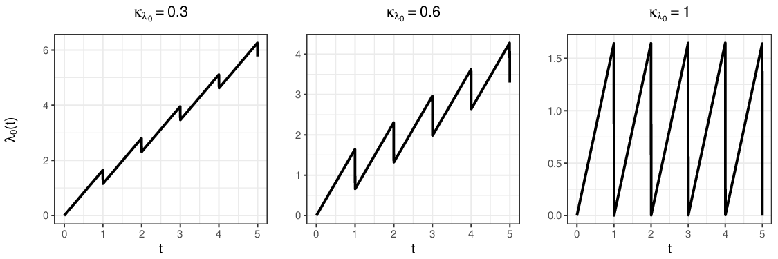
The type-specific failure intensity function for the catastrophic failures, denoted , is modelled as follows
| (12) |
Here we assume a Weibull failure intensity, which is widely used in reliability engineering due to its versatility and relative simplicity [Bobbio et al., 1980; Wang et al., 2000; Wu, 2019], but other choices can be valid. In our model the risk factors do not influence the catastrophic failure mode, however adding this influence is a possible extension of this model.
Maximizing the log-likelihood gives estimates for the model parameters, i.e. and for the baseline hazard, and for the influence of the machine covariates, and and for the catastrophic failures.
Likelihood for minor failure types
The component also contains the failure types. Previously, we incorporated only the distinction between minor and catastrophic failures. Now we handle the different minor failure types. We estimate the parameters of a multinomial logit model which delivers the probabilities for the minor failure types , where [Frees and Valdez, 2008]. Using the observed data, the contribution to the log-likelihood of an observed minor failure type is
| (13) |
Summing over all machines and minor failures gives the full log-likelihood. Following Frees and Valdez, 2008, these probabilities are specified as
| (14) | ||||
where denotes the covariates influencing the failure type probabilities. can include a selection of both fixed and time-dependent covariates, where the time-dependent covariates are evaluated at the failure time. These probabilities specify a multinomial distribution which is typically used to classify multiclass data. If multiple minor failures occur at the same time, they are modelled as a single minor (extra) failure type, e.g. type 3 could be the co-occurrence of a type 1 and a type 2 failure. Maximizing the log-likelihood gives estimates for the parameters driving each minor failure type .11 1 In the R [R Core Team, 2017] package ‘nnet’ [Venables and Ripley, 2002], maximum likelihood estimation for the multinomial logit model is available.
Severity likelihood
The last two components of the decomposition and
deal with the failure and maintenance costs respectively.
We compose a distributional model for the costs using marginal severity distributions on the one hand and a copula for the dependency of costs in case of co-occurring failures on the other hand.
We model the probability density function of the preventive maintenance costs with a positive and right-skewed distribution, e.g. a gamma distribution,
| (15) |
with the location parameter and the scale parameter. We use the following parameterization for the location parameters: , where the link function is chosen in such a way that the location is positive. We include heterogeneity in these costs through a set of contract specific covariates . Once again, these covariates can include a selection of both fixed and time-dependent covariates, where the time-dependent covariates are evaluated at the failure time. Maximizing the log-likelihood gives estimates for . A similar approach can be followed for minor failure costs (with and the catastrophic failure costs (with . We make a distinction between the cost distribution of the minor and catastrophic failures, because they are different in nature. We denote the influencing covariates on the minor and catastrophic failures as and respectively. The parameters of the cost distributions of the minor and catastrophic failures are denoted as , and (with and , and respectively. A copula with positive dependence, e.g. the Frank copula, captures the statistical dependence between the multiple minor failures costs occurring at the same time [Frees and Valdez, 2008]. We opt for a positive dependence since we assume high failure costs in a failure type will induce high failure costs in the other co-occurring failure type.
4.2 From predictive models to pricing
Based on the calibrated predictive models, the break-even price in Equations (5) and (6), can now be determined. We make this explicit by reformulating the break-even price in function of the predictive models, taking into account the risk factors:
| (16) | ||||
where is the predicted number of minor failures within the contract duration and the predicted number of catastrophic failures for machine characteristics and , obtained from the predictive time-to-failure models with likelihood given in Equation (8). Remark that the explicit dependence of the price on the contract duration is omitted from Equation (16), however it is evident that its components are dependent on the contract duration. As the break-even price depends on the machine characteristics, different tariff plans are generated depending on the set of characteristics that are included in the predictive models. As the contract portfolio of the service provider grows, or changes, the models should be re-calibrated to learn from this new data.
Note that the estimates from the predictive models could also be used for other purposes than pricing. An example of this would be data-driven maintenance optimization, where the predictive models for the failure intensity could serve as an input for the optimization of the preventive maintenance interval.
5 Simulation engine and numerical experiment
5.1 Motivation and properties
We develop an engine to generate maintenance and failure data for a portfolio of machines reflecting their heterogeneity induced by the different risk factors. This engine allows testing the performance and adequacy of our analytic models [Bender et al., 2005; Metcalfe and Thompson, 2006; Montez-Rath et al., 2017]. Simulated data provide a controlled environment to study the performance of the methodology in different scenarios preparatory to applying it to real data. At the same time, simulated data provide a recipe for data collection since real data (after cleaning) should have a similar format and features as the simulated data.
The dataset used for pricing should contain the time stamps of failures, including their type and associated costs, the time of preventive maintenance and their costs, together with the machine characteristics. Simulating event occurrences and their associated impact (as in Figure 1) is not straightforward, as extensively documented in the biostatistical literature where the recurrence of events during an individual’s lifetime is studied [Metcalfe and Thompson, 2006; Beyersmann et al., 2009; Hendry, 2014; Jahn-Eimermacher et al., 2015; Pénichoux et al., 2015]. The simulation engine should be capable of handling the following list of analytic ingredients. First, the engine simulates the occurrence of recurrent events over time [Cook and Lawless, 2007; Pénichoux et al., 2015] to generate multiple occurrences of the same type of failure. Next, the engine generates occurrences of different types of events [Beyersmann et al., 2009; Frees and Valdez, 2008] of which some can be terminal, i.e. equivalent to death in the biostatistical setting. The data should also include machine characteristics, which can be time-independent [Metcalfe and Thompson, 2006], e.g. the country of residence, operational environment, operator and maintenance crew skill level, or time-dependent [Hendry, 2014], e.g. temperature, maintenance and service history, which impact failure times, types and costs, and maintenance costs. To introduce non-observable heterogeneity, i.e. not reflected by the observed machine characteristics, the engine could be extended with the inclusion of frailties or random effects [Pénichoux et al., 2015]. Machines may have exactly the same risk factors, but at the same time some of them might fail significantly more. The inclusion of frailties creates additional complexity; since our focus is on observable risk factors, we have not included them in our model. Finally, risk-free intervals [Jahn-Eimermacher et al., 2015], during which no failures can occur, may account for the actual duration of a maintenance intervention.
5.2 Set up of the engine
We generate data for each machine in a portfolio of machines, during an observation time . These machines could be of different types, in which case the machine type should be added as an extra covariate. In our numerical experiment we will assume that all machines have the same type. The observation time of each machine is either 5 years or uniformly distributed between three and five years. We simulate each machine in a time window . Without loss of generality we will consider for all machines. Each machine has a number of characteristics or covariates , where we make a distinction between time-independent and time-dependent covariates. Each machine has 4 fixed covariates, . For the purpose of simulation, we randomly allocate the values with equal probability to the fixed covariates. We adhere to a general specification of the fixed covariates, while in reality these will collect machine-specific risk factors as outlined in Section 1. We let indicate the time-varying covariate whether a type 3 minor failure has occurred,
| (17) |
The time-varying covariate can be seen as a collateral damage of a type 3 failure: i.e. if a type 3 failure occurs, the overall reliability of the machine deteriorates. Other time-varying covariates could represent e.g. the time since last maintenance event, the number of maintenance events in the past year, the cost of the last preventive maintenance, etc.
Next, we determine the number of failure types , with the number of minor failure types, and we additionally consider one catastrophic failure. We consider minor failure types (type 1, type 2 and type 3), of which type 3 is the co-occurrence of failures of type 1 and 2. The number of periodic maintenance actions during the contract duration is determined by fixing the maintenance interval . In our experiment, we let the covariates only impact the distribution of the time-to-failure and failure types, but not the costs, although that should not necessarily be the case. Consequently and , , and and in Equations (10), (14) and (15) respectively. An overview of the simulation parameters can be found in Table 4 in Appendix C.
We provide the pseudo-code of our simulation engine in Algorithm 1, see Appendix B. In what follows we describe how the algorithm generates for each machine failures (times, types and costs), and periodic maintenance actions (and their associated costs) within the observation time .
Failure times
Failure times are generated independent of the failure type by the function getFailureTime(,), where is the covariate vector of machine and the event time of the previous failure on machine . We simulate the failure times making use of failure intensities, see Equations (10) and (12) for minor and catastrophic failures respectively. Recurrent minor failure times as well as a catastrophic (terminal) failure are generated from making use of inverse transform sampling [Metcalfe and Thompson, 2006; Cook and Lawless, 2007; Jahn-Eimermacher et al., 2015; Pénichoux et al., 2015]. To facilitate inverse transform sampling, the time-varying covariates should be piecewise constant functions. The latter is the case for our simulation.
Failure type
For each failure with failure time , the function getFailureType(,) generates the failure type through a two-step process, where is the covariate vector of machine . First, we determine if the failure is minor or catastrophic. These failure types occur with probabilities [Beyersmann et al., 2009],
| (18) | ||||
for a failure at time . Minor and catastrophic failures cannot occur at the same time in the current specification of the model. However, the simulation engine could be extended by introducing an extra event-type capturing the co-occurrence of a minor failure and catastrophic failure with its own specific failure intensity.
Second, the type of a minor failure, i.e. , is generated by sampling from a multinomial distribution [Frees and Valdez, 2008] with the probabilities of Equation (14). Multiple coinciding minor failures are modelled as a single minor failure type, in our set-up type 3 is the co-occurrence of a type 1 and a type 2 failure.
Costs of failure and maintenance
We generate , the costs of the th maintenance, and , the costs of the th failure of type , with the functions getMaintenanceCosts() and getFailureCosts(). Hereto, we simulate from a positive and right-skewed distribution, i.e. a gamma distribution. The specifications of the distributions were introduced in Equation (15). A copula with positive dependence, i.e. the Frank copula, captures the statistical dependence between the costs of minor failures occurring at the same time [Frees and Valdez, 2008].
Figure 4 illustrates the generated event time-lines of three arbitrary machines, which result from our simulation engine.

5.3 Data exploration
Empirical distribution of exposure and covariates
We first explore the distribution of the ‘exposure(-to-risk)’ of our simulated contract portfolio [Denuit et al., 2007]. This quantifies the risk each machine in the dataset is exposed to, expressed in terms of its observation time . Although we use time as the unit of exposure, machine run-time could equally be used. The relative exposure for each machine is
| (19) |
Summing the relative exposures for machines taking the same values in the risk factors leads to Figure 5. Figure 5 (top left panel) illustrates that for our dataset, more than of the total exposure is represented by machines for which five years of data is available. Figure 5 (right panels) shows that each fixed covariate in has equal exposure in each of its values in the dataset, whereas the type 3 minor failure (represented by the time-varying covariate ) is only observed (at least once) in less than of the total exposure.

Influence of the covariates
We explore the influence of the covariates on the number of failures by picturing the empirical failure frequency for specific machine profiles, e.g. machines with . This empirical failure frequency is expressed as the ratio of the number of failures of a specified type and the total exposure, both calculated for the machine profile under consideration. Taking the ratio is necessary to take the exposure (observation time) into account, since more failures are expected when a machine profile is observed for a longer period. Figure 6 illustrates how the covariates influence the failure behaviour for the minor failures, illustrated for minor failure type 1, but have no influence on the catastrophic failures.

5.4 Calibration of the predictive models and resulting pricing schemes
Table 4 (see Appendix C) provides the estimated parameters and their confidence intervals resulting from the calibration of the predictive models using the calibration strategy outlined in Section 4. The confidence intervals follow from the properties of maximum likelihood estimators.
The choice (or availability) of the machine-dependent covariates , , and determines the tariff plan. For a real-life dataset, the relevant covariates have to be obtained by means of variable selection strategies [Henckaerts et al., 2018]. For the purpose of our experiment, however, we assume all covariates are relevant and omit the selection step. In what follows, we introduce three different tariff plans with respective break-even prices and . In tariff plan we do not include any covariates, which means there is no price differentiation and all customers pay the same price. Tariff plan only takes the fixed covariates into account, and tariff plan takes both the fixed and time-dependent covariates into account, see Table 2. We calibrate the predictive models for each combination of covariates taken into consideration.
| failure time | ||||
|---|---|---|---|---|
| failure types | ||||
| costs |
For each machine profile, Figure 7 displays the resulting break-even prices prescribed by the different tariff plans for a contract duration of two years. The different machine profiles arise from the four fixed covariates in vector , taking two different levels each. Additionally, a machine either has experienced a minor failure of type before the start of the contract, , or not, . This leads to different machine profiles upon initiation of the contract, resulting in different prices under tariff plan . Tariff plan does not take into account the time-varying covariate and as such it generates only different prices. Tariff plan returns the same price for every machine profile since it does not consider any risk factors.
Although the average, over all machine profiles, break-even price under all tariff plans is very similar, the difference between the price under tariff and the prices under tariffs and can be quite significant. This effect arises because tariff overcharges low risk machines and undercharges high risk machines. The difference between tariff and is less pronounced since the influence of the time-varying covariate is minor. It is necessary to stress that the price of a one-year contract is not half of the two-year contract prices displayed in Figure 7, nor is the price of a four-year contract double the price of a two-year contract. The price of the contracts is non-homogeneous in time since the failure intensity is non-homogeneous.

In Appendix D (Supplementary material) we provide the results of an extensive simulation study, where we generate multiple portfolios of machines over time (along the recipe in Section 5.2) and calibrate the proposed hierarchical likelihood on each of these simulated datasets. The purpose of this simulation study is to verify the accurracy of the calibration strategy described in Section 4.
6 Model lift: Evaluation of different tariff plans
We evaluate the different tariff plans and introduced in Table 2 for our simulated portfolio of machines by comparing the collected service fees, with the actual, out-of-time collected costs. We divide the machine data in two parts: an in-time training set to calibrate the predictive models and to determine the prices, and an out-of-time set, which returns the actual costs [Goldburd et al., 2016], see Figure 8. With our simulation engine we generate both in-time data (with an observation time of maximum five years), as well as out-of-time data (five extra years data for each machine) with the same simulation settings. We not only measure the accuracy of the tariff plan, i.e. the extent to which the tariff plan (calibrated in-time) covers the actual costs (as observed out-of-time) in the portfolio, but also its capability to identify machine heterogeneity and adapt prices accordingly.
6.1 Accuracy of tariff plans
The loss ratio for a given tariff plan is a measure for tariff accuracy. It is defined as the ratio of the total actual costs realized in the entire contract portfolio over the total collected services fees under the tariff plan. As such, we can express the loss ratio as follows,
| (20) |
where the sum is over all contracts in the portfolio. Table 3 confirms that over a horizon of two years, the three considered tariff plans all have an out-of-time loss ratio close to one. Figure 9 plots the out-of-time loss ratio over time, confirming Table 3 that the loss ratio rapidly stabilizes to a value close to one. That means that at the (aggregated) level of the contract portfolio, all three tariff plans are break-even. Nevertheless, that does not imply that each contract (at the level of the individual machine) is expected to be break-even under the three tariff plans.
| tariff plan | |||
|---|---|---|---|
| loss ratio |

6.2 Capability to differentiate
To measure the capability of a tariff plan to differentiate its prices based on the machine profiles (and their corresponding risk), we use the so-called model lift [Goldburd et al., 2016]. A better capability to differentiate prices implies that the contracts of each machine profile are expected to be break-even, and it prevents adverse selection, as low-risk customers will be offered a lower price than high-risk customers and thus have less incentive to leave.
Quantile plot
The quantile plots in Figure 10 graphically compare the actual, out-of-time, total costs incurred during the contract with the proposed machine-specific break-even price over a two year horizon. For a portfolio of contracts with price for machine , incurred costs and machine characteristics , the quantile plot is obtained by first sorting the contracts in ascending order of price and binning them in equal groups, so-called quantiles; for each bin we then compare the average costs against the corresponding average price. The quantile plots in Figure 10 indicate that tariff plans and succeed in charging a higher price to the more maintenance-heavy contracts. The gap between the average price and average costs for each bin is small, indicating that the contracts in each bin are (close to) break-even on average. Tariff plan sorts the contracts randomly since all contracts have the same price and consequently each bin has a similar average cost. This contrasts to tariffs and , who impose an ordering of the contracts from maintenance-light to maintenance-heavy and as such there is an upward trend in average costs for each quantile. Clearly, under tariff plan , the average maintenance-light contract is profitable, but the average maintenance-heavy contract is loss-making.

Adverse selection
The heterogeneity in maintenance costs of the different contracts is identified by tariff plans and that take into account the risk factors. These tariff plans effectively classify contracts based on their risk and distinguish between maintenance intensive (high risk) versus maintenance light (low risk) contracts. In Figure 10, we can observe that the first 5 quantiles of contracts for tariff plans and have average costs and prices below . We will call these contracts ‘low-risk’ contracts and we will call the 5 last quantiles ‘high-risk’ contracts. Since tariff plan charges all contracts more than , the low-risk customers have an incentive to renege from their contract under tariff . This would leave the service provider, in case he offers tariff plan to all customers, with a portfolio of high-risk contracts only. From Figure 10, we can see that these high-risk contracts have higher average costs than the premium charged by tariff plan . This puts the service provider at risk that he is left with a portfolio that is no longer break-even. In contrast, tariff plans and charge a premium in line with the expected costs of a contract. Therefore, the customers have less incentive to renege on their contract. Moreover, when customers leave, this is not detrimental to the profitability since the lost premiums are in line with the costs, which in that case no longer have to be covered by the service provider.
Lorenz curves and Gini index
A Lorenz curve [Lorenz, 1905] is a tool to compare distributions, frequently used in welfare economics. We use it here to gain insight in the distribution of incurred costs and prices prescribed by the different tariff plans. The Lorenz curve is obtained by sorting the machines in ascending order of price , with the cumulative percentage of the machine population on the abscissa and the cumulative percentage of costs on the ordinate [Frees et al., 2011; Frees et al., 2014]. The larger the gap between the Lorenz curve and the Line of Equality, i.e., the degree line, the better the tariff plan’s capability to reflect heterogeneity between machines via a differentiated price list. The Gini index [Gini, 1912] is twice the area between the Lorenz Curve and the Line of Equality. Figure 11 shows the Lorenz curves and corresponding Gini coefficients for the different tariff plans. The larger Gini index of tariff plans and indicate that they outperform tariff plan in differentiating between low-risk and high-risk contracts (which is expected since tariff plan charges every customer the same price). Remark that we can construct the Lorenz curve for any tariff plan, since it only requires prices and costs as input. As such, we could use the Lorenz curve and Gini index to evaluate our pricing methodology against current pricing practices.

Ordered Lorenz curves and Gini index
As an extension to the Lorenz curves, Frees et al., 2011; Frees et al., 2014 introduce ordered Lorenz curves. These consider whether an alternative tariff plan is preferred over the current plan because it is better capable to differentiate prices. The relativity for contract is defined by the ratio of the alternative tariff plan over the current plan,
| (21) |
When both tariff plans cover the expected costs, the average over all contracts will be close to one. A low relativity indicates that price is lower than , suggesting that tariff plan is more competitive than tariff for contract , and contract is potentially lost to a competitor with tariff plan . A high value for contract indicates that is underpriced and could indicate potential losses when adopting tariff . Hence, the more contracts with a relativity differing from 1, the worse tariff plan is compared to . This interpretation of the relativities assumes that prices are a more accurate representation of the actual costs than .
To set up the ordered Lorenz curve, the contracts in the portfolio are ordered in increasing values of . The distribution of the current prices and distribution of the costs can then be calculated as:
| (22) |
with the indicator function, returning 1 if the argument is true and zero otherwise.
The graph
then defines the ordered Lorenz curve [Frees et al., 2011; Frees et al., 2014].
The associated Gini index is again twice the area between the Lorenz curve and the Line of Equality.
Figure 12 shows a two-way comparison of the three tariff plans resulting in six ordered Lorenz curves. As shown in the top left panel for tariff plan , the contracts with lowest are priced too high with respect to their costs (i.e., contribute disproportional to the total price than to the total costs), and vice versa for the contracts with high . This results in a convex curve below the Line of Equality. An ordered Lorenz curve corresponding to the Line of Equality (for instance in the bottom panels) indicates that the cumulative percentage of the costs equals the cumulative percentage of the prices, both in increasing relativities. Consequently, the alternative tariff is not preferred over the current tariff . Tariff plan is preferred over in case the ordered Lorenz curve is further away from the Line of Equality, indicating that more contracts have a relativity further away from 1. The more convex the ordered Lorenz curve, the more tariff can recognize deficiencies in tariff . The latter is equivalent with a larger Gini index. In this sense tariff plans and both clearly dominate scheme . The advantage of tariff over is, however, minor.

7 Conclusions
We study full-service maintenance agreements that cover all maintenance costs over a predetermined time horizon in exchange for a fixed premium. The stochastic and machine-dependent nature of the maintenance costs renders the determination of the premium challenging for the service provider. Inspired by insurance pricing, we use predictive analytics to determine the break-even price based on customer- and machine-dependent characteristics. We build a simulation engine to simulate data that reflect this heterogeneity in maintenance occurrences and their costs and we show the economic value of price differentiation.
We demonstrate how price differentiation can help withstand adverse selection in case of a machine population with diverse maintenance costs. We provide visual tools, such as quantile plots and (ordered) Lorenz curves, and quantitative measures, i.e. the Gini coefficient, to provide insight in the performance of the resulting tariff plans with respect to the heterogeneity of the machine population and with respect to each other.
We propose a couple of directions for further research, some of which are relaxations of the assumptions made in this paper. First, we assumed the independence between occurrence, or frequency, of failures and their associated costs. The insurance pricing literature proposes to deal with dependence between occurrence and costs of claims by making use of for instance copulas. This approach could also be transferred to pricing full-service maintenance contracts. Second, we have demonstrated our approach on simulated data. Although our simulation engine reflects a lot of properties of real-world data, a validation of our approach on a real dataset seems a logical next step. Third, our method relies on observable and measurable covariates to classify machines. We assume that most of the heterogeneity between machines is captured by these measurable covariates or risk factors. In the event that some heterogeneity is not explained by the observed covariates, we could rely on frailties, also known as random effects, to model the unobserved heterogeneity.
Acknowledgments
The authors thank the anonymous referees and the editor for useful comments which led to significant improvements of the paper.
References
- Bakshi et al., [2015] Bakshi, N., Kim, S.-H., and Savva, N. (2015). Signaling new product reliability with after-sales service contracts. Management Science, 61(8):1812–1829.
- Barabadi, [2012] Barabadi, A. (2012). Reliability and spare parts provision considering operational environment: A case study. International Journal of Performability Engineering, 8(5).
- Barabadi et al., [2014] Barabadi, A., Barabady, J., and Markeset, T. (2014). Application of reliability models with covariates in spare part prediction and optimization–a case study. Reliability Engineering & System Safety, 123:1–7.
- Barlow and Hunter, [1960] Barlow, R. and Hunter, L. (1960). Optimum preventive maintenance policies. Operations Research, 8(1):90–100.
- Bender et al., [2005] Bender, R., Augustin, T., and Blettner, M. (2005). Generating survival times to simulate Cox proportional hazards models. Statistics in medicine, 24(11):1713–1723.
- Bertsimas and Kallus, [2020] Bertsimas, D. and Kallus, N. (2020). From predictive to prescriptive analytics. Management Science, 66(3):1025–1044.
- Beyersmann et al., [2009] Beyersmann, J., Latouche, A., Buchholz, A., and Schumacher, M. (2009). Simulating competing risks data in survival analysis. Statistics in medicine, 28(6):956–971.
- Bobbio et al., [1980] Bobbio, A., Cumani, A., Premoli, A., and Saracco, O. (1980). Modeling and identification of nonexponential distributions by homogeneous Markov processes. In Proc. of the Sixth Advances in Reliability Symposium.
- Chan et al., [2018] Chan, T. H., de Véricourt, F., and Besbes, O. (2018). Contracting in medical equipment maintenance services: An empirical investigation. Management Science, 65(3):1136–1150.
- Cook and Lawless, [2007] Cook, R. J. and Lawless, J. (2007). The statistical analysis of recurrent events. Springer Science & Business Media.
- Cox, [1975] Cox, D. R. (1975). Partial likelihood. Biometrika, 62(2):269–276.
- Czado et al., [2012] Czado, C., Kastenmeier, R., Brechmann, E. C., and Min, A. (2012). A mixed copula model for insurance claims and claim sizes. Scandinavian Actuarial Journal, 2012(4):278–305.
- De Jong et al., [2008] De Jong, P., Heller, G. Z., et al. (2008). Generalized linear models for insurance data, volume 10. Cambridge University Press Cambridge.
- Denuit et al., [2007] Denuit, M., Maréchal, X., Pitrebois, S., and Walhin, J.-F. (2007). Actuarial modelling of claim counts: Risk classification, credibility and bonus-malus systems. John Wiley & Sons.
- Doyen and Gaudoin, [2011] Doyen, L. and Gaudoin, O. (2011). Modeling and assessment of aging and efficiency of corrective and planned preventive maintenance. IEEE Transactions on Reliability, 60(4):759–769.
- Frees et al., [2011] Frees, E. W., Meyers, G., and Cummings, A. D. (2011). Summarizing insurance scores using a Gini index. Journal of the American Statistical Association, 106(495):1085–1098.
- Frees et al., [2014] Frees, E. W., Meyers, G., and Cummings, A. D. (2014). Insurance ratemaking and a Gini index. Journal of Risk and Insurance, 81(2):335–366.
- Frees and Valdez, [2008] Frees, E. W. and Valdez, E. A. (2008). Hierarchical insurance claims modeling. Journal of the American Statistical Association, 103(484):1457–1469.
- Gebauer et al., [2005] Gebauer, H., Fleisch, E., and Friedli, T. (2005). Overcoming the service paradox in manufacturing companies. European management journal, 23(1):14–26.
- Gini, [1912] Gini, C. (1912). Italian: Variabilità e mutabilità. Variability and Mutability’, C. Cuppini, Bologna.
- Goldburd et al., [2016] Goldburd, M., Khare, A., and Tevet, D. (2016). Generalized linear models for insurance rating. Casualty Actuarial Society, CAS Monographs Series, (5).
- Gschlößl and Czado, [2007] Gschlößl, S. and Czado, C. (2007). Spatial modelling of claim frequency and claim size in non-life insurance. Scandinavian Actuarial Journal, 2007(3):202–225.
- Guajardo et al., [2012] Guajardo, J. A., Cohen, M. A., Kim, S.-H., and Netessine (2012). Impact of performance-based contracting on product reliability: An empirical analysis. Management Science, 58(5):961–979.
- Hancock et al., [2005] Hancock, M. Q., John, R. H., and Wojcik, P. J. (2005). Better B2B selling. McKinsey Quarterly, 38(3):15.
- Henckaerts et al., [2018] Henckaerts, R., Antonio, K., Clijsters, M., and Verbelen, R. (2018). A data driven binning strategy for the construction of insurance tariff classes. Scandinavian Actuarial Journal, 2018(8):681–705.
- Hendry, [2014] Hendry, D. J. (2014). Data generation for the Cox proportional hazards model with time-dependent covariates: a method for medical researchers. Statistics in medicine, 33(3):436–454.
- Huber and Spinler, [2012] Huber, S. and Spinler, S. (2012). Pricing of full-service repair contracts. European Journal of Operational Research, 222(1):113–121.
- Huber and Spinler, [2014] Huber, S. and Spinler, S. (2014). Pricing of full-service repair contracts with learning, optimized maintenance, and information asymmetry. Decision Sciences, 45(4):791–815.
- Jahn-Eimermacher et al., [2015] Jahn-Eimermacher, A., Ingel, K., Ozga, A.-K., Preussler, S., and Binder, H. (2015). Simulating recurrent event data with hazard functions defined on a total time scale. BMC medical research methodology, 15(1):16.
- Kaas et al., [2008] Kaas, R., Goovaerts, M., Dhaene, J., and Denuit, M. (2008). Modern actuarial risk theory: using R, volume 128. Springer Science & Business Media.
- Kijima, [1989] Kijima, M. (1989). Some results for repairable systems with general repair. Journal of Applied probability, 26(1):89–102.
- Kim et al., [2017] Kim, S.-H., Cohen, M. A., and Netessine, S. (2017). Reliability or inventory? an analysis of performance-based contracts for product support services. In Handbook of Information Exchange in Supply Chain Management, pages 65–88. Springer.
- Lindqvist et al., [2006] Lindqvist, B. H. et al. (2006). On the statistical modeling and analysis of repairable systems. Statistical science, 21(4):532–551.
- Lorenz, [1905] Lorenz, M. O. (1905). Methods of measuring the concentration of wealth. Publications of the American statistical association, 9(70):209–219.
- [35] Luo, M. and Wu, S. (2018a). A mean-variance optimisation approach to collectively pricing warranty policies. International Journal of Production Economics, 196:101–112.
- [36] Luo, M. and Wu, S. (2018b). A value-at-risk approach to optimisation of warranty policy. European Journal of Operational Research, 267(2):513 – 522.
- Metcalfe and Thompson, [2006] Metcalfe, C. and Thompson, S. G. (2006). The importance of varying the event generation process in simulation studies of statistical methods for recurrent events. Statistics in medicine, 25(1):165–179.
- Montez-Rath et al., [2017] Montez-Rath, M. E., Kapphahn, K., Mathur, M. B., Purington, N., Joyce, V. R., and Desai, M. (2017). Simulating realistically complex comparative effectiveness studies with time-varying covariates and right-censored outcomes. arXiv preprint arXiv:1709.10074.
- Nouri Qarahasanlou et al., [2016] Nouri Qarahasanlou, A., Ataei, M., Khalokakaie, R., Ghodrati, B., and Jafarei, R. (2016). Tire demand planning based on reliability and operating environment. Int. Journal of Mining & Geo-Engineering, 50(2):239–248.
- Pénichoux et al., [2015] Pénichoux, J., Moreau, T., and Latouche, A. (2015). Simulating recurrent events that mimic actual data: a review of the literature with emphasis on event-dependence. arXiv preprint arXiv:1503.05798.
- Poppe et al., [2018] Poppe, J., Boute, R. N., and Lambrecht, M. R. (2018). A hybrid condition-based maintenance policy for continuously monitored components with two degradation thresholds. European Journal of Operational Research, 268(2):515–532.
- R Core Team, [2017] R Core Team (2017). R: A Language and Environment for Statistical Computing. R Foundation for Statistical Computing, Vienna, Austria.
- Rapaccini, [2015] Rapaccini, M. (2015). Pricing strategies of service offerings in manufacturing companies: a literature review and empirical investigation. Production Planning & Control, 26(14-15):1247–1263.
- Rebaiaia et al., [2017] Rebaiaia, M. L., Ait-kadi, D., and Jamshidi, A. (2017). Periodic replacement strategies: optimality conditions and numerical performance comparisons. International Journal of Production Research, 55(23):7135–7152.
- Sawhney et al., [2003] Sawhney, M., Balasubramanian, S., and Krishnan, V. V. (2003). Creating growth with services. MIT Sloan management review, 45(2):34–44.
- Sheu et al., [2012] Sheu, S.-H., Li, S.-H., and Chang, C.-C. (2012). A generalised maintenance policy with age-dependent minimal repair cost for a system subject to shocks under periodic overhaul. International Journal of Systems Science, 43(6):1007–1013.
- Ulaga and Reinartz, [2011] Ulaga, W. and Reinartz, W. J. (2011). Hybrid offerings: how manufacturing firms combine goods and services successfully. Journal of marketing, 75(6):5–23.
- Venables and Ripley, [2002] Venables, W. N. and Ripley, B. D. (2002). Modern Applied Statistics with S. Springer, New York, fourth edition. ISBN 0-387-95457-0.
- Verbelen et al., [2018] Verbelen, R., Antonio, K., and Claeskens, G. (2018). Unravelling the predictive power of telematics data in car insurance pricing. Journal of the Royal Statistical Society: Series C (Applied Statistics), 67(5):1275–1304.
- Visnjic and Van Looy, [2013] Visnjic, I. and Van Looy, B. (2013). Servitization: Disentangling the impact of service business model innovation on manufacturing firm performance. Journal of Operations Management, 31(4):169–180.
- Wang et al., [2000] Wang, W., Scarf, P., and Smith, M. (2000). On the application of a model of condition-based maintenance. Journal of the Operational Research Society, 51(11):1218–1227.
- Wu, [2019] Wu, S. (2019). A failure process model with the exponential smoothing of intensity functions. European Journal of Operational Research, 275(2):502–513.
- Wu and Zuo, [2010] Wu, S. and Zuo, M. J. (2010). Linear and nonlinear preventive maintenance models. IEEE transactions on reliability, 59(1):242 – 249.
Appendix A List Of Notations
Appendix B Pseudo-code of the simulation engine
Appendix C Results of the calibration of the predictive models in our numerical experiment
We present the calibrated parameters and their -confidence intervals of the predictive models for the simulation settings as introduced in Section 5 in Table 4. These are obtained by the calibration of a single simulation run.
| Parameter | Simulation | Calibration | |
|---|---|---|---|
| estimate | conf. | ||
| interval | |||
| - | - | ||
| Pricing scheme | Pricing scheme | Pricing scheme | |||
|---|---|---|---|---|---|
| estimate | conf. | estimate | conf. | estimate | conf. |
| interval | interval | interval | |||
| - | - | - | - | - | - |
| - | - | ||||
| - | - | ||||
| - | - | ||||
| - | - | ||||
| - | - | - | - | ||
| - | - | ||||
| - | - | ||||
| - | - | ||||
| - | - | ||||
| - | - | ||||
| - | - | ||||
| - | - | ||||
| - | - | ||||
Appendix D Simulation study to verify the calibration method
To verify the calibration of our predictive models, we simulate replications of the simulation setting described in Section 5. The number of machines for this verification is equal to , in contrast to in Section 5, that we used to illustrate our pricing methodology. Each replication leads a single estimate for the simulation parameters. Consequently it is possible to compare these estimates with the simulation parameters by means of a boxplot. The boxplots for the time-to-failure model parameters, multinomial distribution parameters and the costs distribution parameters can be found on Figures 13, 14 and 15 respectively and the averages of the estimates in Table 5. The average estimates are very close to the simulation parameters and this confirms the accuracy of calibration strategy.
| parameter | simulation | average |
|---|---|---|
| value | estimate | |


