跳到论文正文
W Papers独立论文阅读器 arXiv:2007.01012 论文正文 计算阅读时间 · 0%
引用这篇论文根据当前论文元数据生成,正式投稿前建议核对。


License: arXiv.org perpetual non-exclusive license
arXiv:2007.01012v2 [cs.LG] 27 Jul 2020

Consistent Structured Prediction with Max-Min Margin Markov Networks

Alex Nowak-Vila Affiliation: INRIA - Département d’Informatique de l’Ecole Normale Supérieure, PSL Research University Correspondence to: alex.nowak-vila@inria.fr    Francis Bach Affiliation: INRIA - Département d’Informatique de l’Ecole Normale Supérieure, PSL Research University    Alessandro Rudi Affiliation: INRIA - Département d’Informatique de l’Ecole Normale Supérieure, PSL Research University
Abstract

Max-margin methods for binary classification such as the support vector machine (SVM) have been extended to the structured prediction setting under the name of max-margin Markov networks (M3​N\operatorname{M^{3}N}), or more generally structural SVMs. Unfortunately, these methods are statistically inconsistent when the relationship between inputs and labels is far from deterministic. We overcome such limitations by defining the learning problem in terms of a “max-min” margin formulation, naming the resulting method max-min margin Markov networks (M4​N\operatorname{M^{4}N}). We prove consistency and finite sample generalization bounds for M4​N\operatorname{M^{4}N} and provide an explicit algorithm to compute the estimator. The algorithm achieves a generalization error of O⁡(1/n)O(1/\sqrt{n}) for a total cost of O⁡(n)O(n) projection-oracle calls (which have at most the same cost as the max-oracle from M3​N\operatorname{M^{3}N}). Experiments on multi-class classification, ordinal regression, sequence prediction and ranking demonstrate the effectiveness of the proposed method.

Keywords: 
Machine Learning, ICML

1 Introduction

Many classification tasks in machine learning lie beyond the classical binary and multi-class classification settings. In those tasks, the output elements are structured objects made of interdependent parts, such as sequences in natural language processing (Smith 2011), images in computer vision (Nowozin & Lampert 2011), permutations in ranking or matching problems (Caetano et al. 2009) to name just a few (BakIr et al. 2007). The structured prediction setting has two key properties that makes it radically different from multi-class classification, namely, the exponential growth of the size of the output space with the number of its parts, and the cost-sensitive nature of the learning task, as prediction mistakes are not equally costly. In sequence prediction, for instance, the number of possible outputs grows exponentially with the length of the sequences, and predicting a sequence with one incorrect character is better than predicting the whole sequence wrong.

Classical approaches in binary classification such as the non-smooth support vector machine (SVM), and the smooth logistic and quadratic plug-in classifiers have been extended to the structured setting under the name of max-margin Markov networks (M3​N\operatorname{M^{3}N}) (Taskar et al. 2004) (or more generally structural SVM (SSVM) (Tsochantaridis et al. 2005)), conditional random fields (CRFs) (Lafferty et al. 2001) and quadratic surrogate (QS) (Ciliberto et al. 2016; Ciliberto et al. 2019), respectively. Theoretical properties of CRF and QS are well-understood. In particular, it is possible to obtain finite-sample generalization bounds of the resulting estimator on the cost-sensitive structured loss (Nowak-Vila et al. 2019a). Unfortunately, these guarantees are not satisfied by M3​N\operatorname{M^{3}N}s even though the method is based on an upper bound of the loss. More precisely, it is known that the upper bound can be not tight (and lead to inconsistent estimation) when the relationship between input and output labels is far from deterministic (Liu 2007), which it is essentially always the case in structured prediction due to the exponentially large output space. This means that the estimator does not converge to the minimizer of the problem leading to inconsistency.

Recently, a line of work (Fathony et al. 2016; Fathony et al. 2018a; Fathony et al. 2018b; Fathony et al. 2018c) proposed a consistent method based on an adversarial game formulation on the structured problem. However, their analysis does not allow to get generalization bounds and their proposed algorithm is specific for every setting with at least a complexity of O⁡(n2)O(n^{2}) to obtain optimal statistical error when learning from nn samples. In this paper, we derive this method in the generic structured output setting from first principles coming from the binary SVM. We name this method max-min margin Markov networks (M4​N\operatorname{M^{4}N}), as it is based on a correction of the max-margin of M3​N\operatorname{M^{3}N} to a ‘max-min’ margin. The proposed algorithm has essentially the same complexity as state-of-the-art methods for M3​N\operatorname{M^{3}N} on the regularized empirical risk minimization problem, but it comes with consistency guarantees and finite sample generalization bounds on the discrete structured prediction loss, with constants that are polynomial in the number of parts of the structured object and do not scale as the size of the output space. More precisely, the algorithm requires a constant number of projection-oracles at every iteration, each of them having at most the same cost as the max-oracle of M3​N\operatorname{M^{3}N}. We also provide experiments on multiple tasks such as multi-class classification, ordinal regression, sequence prediction and ranking, showing the effectiveness of the algorithm. We make the following contributions:

  • -

    We introduce max-min margin Markov networks (M4​N\operatorname{M^{4}N}) in definition 3.1 and prove consistency, linear calibration and finite sample generalization bounds for the regularized ERM estimator in Thms. 3.2, 3.3 and 3.4, respectively.

  • -

    We generalize the BCFW algorithm (Lacoste-Julien et al. 2013) used for M3​N\operatorname{M^{3}N}s to M4​N\operatorname{M^{4}N}s and solve the max-min oracle iteratively with projection oracle calls using Saddle Point Mirror Prox (Nemirovski 2004). We prove bounds on the expected duality gap of the regularized ERM problem in theorem 5.1 and statistical bounds in theorem 5.2.

  • -

    In section 6, we perform a thorough experimental analysis of the proposed method on classical unstructured and structured prediction settings.

2 Surrogate Methods for Classification

In this section, we review the first principles underlying surrogate methods starting from binary classification and moving into structured prediction. We put special attention to the difference between plug-in (e.g., logistic) and direct (e.g., SVM) classifiers to show that while there is a complete picture in the binary setting, existing direct classifiers in structured prediction lack the basic properties of binary SVMs. The first goal of this paper is to complete this picture in the structured output setting.

2.1 A Motivation from Binary Classification

Let 𝒴={−1,1}\mathcal{Y}=\{-1,1\} and (x1,y1),…,(xn,yn)(x_{1},y_{1}),\ldots,(x_{n},y_{n}) be nn input-output pairs sampled from a distribution ρ\rho. The goal in binary classification is to estimate a binary-valued function f⋆:𝒳→𝒴f^{\star}:\mathcal{X}\xrightarrow{}\mathcal{Y} that minimizes the classification error

ℰ⁡(f)=𝔼(x,y)∼ρ⁡1​(f⁡(x)≠y).\textstyle{\mathcal{E}(f)=\operatorname{\mathbb{E}}_{(x,y)\sim\rho}1(f(x)\neq y)}.

We can avoid working with binary-valued functions by considering instead real-valued functions g:𝒳→ℝg:\mathcal{X}\xrightarrow{}\mathbb{R} and use the prediction model f⁡(x)=d∘g⁡(x)   .  .  =sign⁡(g⁡(x))f(x)=d\circ g(x)\mathrel{\vbox{\hbox{\scriptsize.}\hbox{\scriptsize.}}}=\operatorname{sign}(g(x)) (Bartlett et al. 2006) where dd stands for decoding. The resulting problem reads

g⋆∈arg​ming:𝒳→ℝℰ(d∘g).g^{\star}\in\operatorname*{arg\;min}_{g:\mathcal{X}\rightarrow\mathbb{R}}~\mathcal{E}(d\circ g). (1)

Unfortunately, directly estimating a g⋆g^{\star} from (1) is intractable for many classes of functions (Arora et al. 1997).

Convex surrogate methods.

The source of intractability of minimizing the classification error (1) comes from the discreteness and non-convexity of the loss. The idea of surrogate methods (Bartlett et al. 2006) is to consider a convex surrogate loss S:ℝ×𝒴→ℝS:\mathbb{R}\times\mathcal{Y}\rightarrow\mathbb{R} such that g⋆g^{\star} can be written as

g⋆=arg​ming:𝒳→ℝℛ(g)   .  .  =𝔼(x,y)∼ρS(g(x),y).g^{\star}=\operatorname*{arg\;min}_{g:\mathcal{X}\xrightarrow{}\mathbb{R}}~\mathcal{R}(g)\mathrel{\vbox{\hbox{\scriptsize.}\hbox{\scriptsize.}}}=\operatorname{\mathbb{E}}_{(x,y)\sim\rho}S(g(x),y). (2)

In this case, g⋆g^{\star} can be tractably estimated from nn samples over a family of functions 𝒢\mathcal{G} using regularized ERM. The resulting estimator gng_{n} has the form

gn=arg​ming∈𝒢⁡1n​∑i=1nS⁡(g⁡(xi),yi)+λn2​‖g‖𝒢2,g_{n}=\operatorname*{arg\;min}_{g\in\mathcal{G}}~\frac{1}{n}\sum_{i=1}^{n}S(g(x_{i}),y_{i})+\frac{\lambda_{n}}{2}\|g\|_{\mathcal{G}}^{2}, (3)

where λn>0\lambda_{n}>0 is the regularization parameter and ∥⋅∥𝒢\|\cdot\|_{\mathcal{G}} is the norm associated to the hypothesis space 𝒢\mathcal{G}. If not stated explicitly, our analysis of the surrogate method holds for any function space, such as reproducing kernel Hilbert spaces (RKHS) (Aronszajn 1950) or neural networks (LeCun et al. 2015), where we lose global theoretical convergence guarantees of problem (3).

The classical theoretical requirements of such a surrogate strategy are Fisher consistency (i) and a comparison inequality (ii):

(i)ℰ⁡(f⋆)=ℰ⁡(d∘g⋆)(ii)ζ⁡(ℰ⁡(d∘g)−ℰ⁡(f⋆))≤ℛ⁡(g)−ℛ⁡(g⋆),\begin{array}[]{ll}\text{(i)}&\mathcal{E}(f^{\star})=\mathcal{E}(d\circ g^{\star})\\ \text{(ii)}&\zeta(\mathcal{E}(d\circ g)-\mathcal{E}(f^{\star}))\leq\mathcal{R}(g)-\mathcal{R}(g^{\star}),\end{array}

for all measurable functions gg, where ζ:ℝ+→ℝ+\zeta:\mathbb{R}_{+}\xrightarrow{}\mathbb{R}_{+} is such that ζ⁡(ε)→0\zeta(\varepsilon)\to 0 when ε→0\varepsilon\to 0. Note that Condition (i) is equivalent to (1). Condition (ii) is needed to prove consistency results, to show that ℛ⁡(g)→ℛ⁡(g⋆)\mathcal{R}(g)\rightarrow\mathcal{R}(g^{\star}) implies ℰ⁡(d∘g)→ℰ⁡(f⋆)\mathcal{E}(d\circ g)\rightarrow\mathcal{E}(f^{\star}). The existence of ζ\zeta satisfying (ii) is derived from (i) and the continuity and lower boundedness of S⁡(v,y)S(v,y), see Thm. 3 by (Zhang 2004). Even though the explicit form of ζ\zeta is not needed for a consistency analysis, it is necessary to prove finite sample generalization bounds, as it is the mathematical object relating the suboptimality of the surrogate problem to the suboptimality of the original task. Note that the larger ζ⁡(ε)\zeta(\varepsilon), the better.

Plug-in classifiers.

It is known that (i) is satisfied for any function g⋆g^{\star} that continuously depends on the conditional probability ρ⁡(1|x)\rho(1|x) as g⋆​(x)   .  .  =t⁡(ρ⁡(1|x))g^{\star}(x)\mathrel{\vbox{\hbox{\scriptsize.}\hbox{\scriptsize.}}}=t(\rho(1|x)), where t:ℝ→ℝt:\mathbb{R}\rightarrow\mathbb{R} is a suitable continuous bijection of the real line11 1 It must satisfy (u−1/2)​t​(u−1/2)≥0(u-1/2)t(u-1/2)\geq 0 for all u∈ℝu\in\mathbb{R}.. In this case, eq. 2 can be satisfied using smooth losses. Some examples are the logistic loss log⁡(1+e−y​v)\log(1+e^{-yv}), the squared hinge loss max⁡(0,1−y​v)2\max(0,1-yv)^{2} and the exponential loss e−y​ve^{-yv}. In this case, the convexity and smoothness of S⁡(⋅,y)S(\cdot,y) imply that (ii) is satisfied with ζ⁡(ε)∼ε2\zeta(\varepsilon)\sim\varepsilon^{2} (Bartlett et al. 2006). Combining this with standard convergence results of regularized ERM estimators gng_{n} on RKHS, the resulting statistical rates are of the form 𝔼ℰ(d∘gn)−ℰ(f⋆)∼∥g⋆∥𝒢n−1/4\operatorname{\mathbb{E}}\mathcal{E}(d\circ g_{n})-\mathcal{E}(f^{\star})\sim\|g^{\star}\|_{\mathcal{G}}n^{-1/4}. Even if the binary learning problem is easy, g⋆g^{\star} can be highly non-smooth away from the decision boundary, resulting in large ‖g⋆‖𝒢\|g^{\star}\|_{\mathcal{G}}. It is known that the dependence on the number of samples can be improved under low noise conditions (Audibert & Tsybakov 2007).

Support vector machines (SVM).

Plug-in classifiers indirectly estimate the conditional probability as ρ⁡(1|x)=t−1​(g⋆​(x))\rho(1|x)=t^{-1}(g^{\star}(x)), which is more than just falling in the right binary decision set. SVMs directly tackle the classification task by estimating g⋆   .  .  =f⋆=sign⁡(ρ⁡(1|x)−1/2)g^{\star}\mathrel{\vbox{\hbox{\scriptsize.}\hbox{\scriptsize.}}}=f^{\star}=\operatorname{sign}(\rho(1|x)-1/2). In this case, the non-smooth hinge loss S⁡(v,y)=max⁡(0,1−y​v)S(v,y)=\max(0,1-yv) satisfies (2). Moreover, (ii) is satisfied with ζ⁡(ε)=ε\zeta(\varepsilon)=\varepsilon and statistical rates are of the form 𝔼ℰ(d∘g^n)−ℰ(f⋆)∼∥f⋆∥𝒢n−1/2\operatorname{\mathbb{E}}\mathcal{E}(d\circ\widehat{g}_{n})-\mathcal{E}(f^{\star})\sim\|f^{\star}\|_{\mathcal{G}}n^{-1/2}. Note that f⋆f^{\star} is piece-wise constant on the support of ρ\rho, but it can be shown f⋆∈𝒢f^{\star}\in\mathcal{G}, (i.e., ‖f⋆‖𝒢<∞\|f^{\star}\|_{\mathcal{G}}<\infty), for standard hypothesis spaces 𝒢{\mathcal{G}} such as Sobolev spaces with input space ℝd\mathbb{R}^{d} and smoothness s>d/2s>d/2 under low noise conditions (Pillaud-Vivien et al. 2018b).

2.2 Structured Prediction Setting

In binary classification, the output data are naturally embedded in ℝ\mathbb{R} as 𝒴={−1,1}⊂ℝ\mathcal{Y}=\{-1,1\}\subset\mathbb{R}. However, as this is not necessarily the case in structured prediction, it is classical (Taskar et al. 2005) to represent the output with an embedding φ:𝒴→ℝk\varphi:\mathcal{Y}\rightarrow\mathbb{R}^{k} encoding the parts structure with k≪|𝒴|k\ll|\mathcal{Y}|. Let g:𝒳→ℝkg:\mathcal{X}\rightarrow\mathbb{R}^{k} and define the following linear prediction model

f⁡(x)=d∘g⁡(x)   .  .  =arg​maxy∈𝒴⁡φ​(y)⊤​g​(x).\textstyle{f(x)=d\circ g(x)\mathrel{\vbox{\hbox{\scriptsize.}\hbox{\scriptsize.}}}=\operatorname*{arg\;max}_{y\in\mathcal{Y}}~\varphi(y)^{\top}g(x)}. (4)

The above decoding (4) corresponds to the classical linear prediction model over factorized joint features Φ⁡(x,y)=φ⁡(y)⊗Φ⁡(x)\Phi(x,y)=\varphi(y)\otimes\Phi(x) when g⁡(x)g(x) is linear in some input features Φ⁡(x)\Phi(x) (BakIr et al. 2007). The form in (4) is required to perform the consistency analysis but the algorithm developed in section 5 can be readily extended to joint features that do not factorize. Non-linear prediction models have been recently proposed by (Belanger & McCallum 2016), but this is out of the scope of this paper.

Let L:𝒴×𝒴→ℝL:\mathcal{Y}\times\mathcal{Y}\rightarrow\mathbb{R} be a loss function between structured outputs encoding the cost-sensitivity of predictions. For instance, it is common to take LL to be the Hamming loss over the parts of the structured object. The goal in structured prediction is to estimate f⋆:𝒳→𝒴f^{\star}:\mathcal{X}\xrightarrow{}\mathcal{Y} that minimizes the expected risk:

ℰ⁡(f)=𝔼(x,y)∼ρ⁡L⁡(f⁡(x),y).\mathcal{E}(f)=\operatorname{\mathbb{E}}_{(x,y)\sim\rho}L(f(x),y). (5)

Loss-decoding compatibility.

It is classical to assume that the loss decomposes over the structured output parts (Joachims 2006). This can be generalized as the following affine decomposition of the loss (Ramaswamy et al. 2013; Nowak-Vila et al. 2019b)

L⁡(y,y′)=φ​(y)⊤​A​φ​(y′)+a,L(y,y^{\prime})=\varphi(y)^{\top}A\varphi(y^{\prime})+a, (6)

for a matrix A∈ℝk×kA\in\mathbb{R}^{k\times k} and scalar a∈ℝa\in\mathbb{R}. Indeed, assumption (6) together with the tractability of (4) is essentially equivalent to the tractability of loss-augmented inference in structural SVMs (Joachims 2006). For the sake of notation, we drop the constant aa and work with the ‘centered’ loss L⁡(y,y′)−aL(y,y^{\prime})-a. We provide some examples below.

Example 2.1 (Structured prediction with factor graphs).

Let 𝒴=[R]M\mathcal{Y}=[R]^{M} be the set of objects made of MM parts, each in a vocabulary of size RR. In order to model interdependence between different parts, we consider embeddings that decompose over (overlapping) subsets of indices α⊆{1,…,M}\alpha\subseteq\{1,\ldots,M\} (Taskar et al. 2004) as φ⁡(y)=(φα​(yα))α\varphi(y)=(\varphi_{\alpha}(y_{\alpha}))_{\alpha}. More precisely, the prediction model corresponds to

arg​maxy∈𝒴∑αφα(yα)⊤vα,\textstyle{\operatorname*{arg\;max}_{y\in\mathcal{Y}}~\sum_{\alpha}\varphi_{\alpha}(y_{\alpha})^{\top}v_{\alpha}}, (7)

where φα​(yα)=eyα∈ℝR|α|\varphi_{\alpha}(y_{\alpha})=e_{y_{\alpha}}\in\mathbb{R}^{R^{|\alpha|}} with eje_{j} being the jj-th vector of the canonical basis and the dimension of the full-embedding φ\varphi is k=∑αR|α|≪|𝒴|=RMk=\sum_{\alpha}R^{|\alpha|}\ll|\mathcal{Y}|=R^{M}. It is common (Tsochantaridis et al. 2005) to assume that the loss decomposes additively over the coordinates as L⁡(y,y′)=1M​∑m=1Lm​(ym,ym′)L(y,y^{\prime})=\frac{1}{M}\sum_{m=1}L_{m}(y_{m},y_{m}^{\prime}) and so the matrix AA associated to the loss decomposition of LL is low-rank. Problem (7) can be solved efficiently for low tree-width structures using the junction-tree algorithm (Wainwright & Jordan 2008). More specifically, if the objects are sequences with embeddings modelling individual and adjacent pairwise characters, Problem (7) can be solved in time O⁡(M​R2)O(MR^{2}) using the Viterbi algorithm (Viterbi 1967).

Example 2.2 (Ranking and matching).

The output space is the group of permutations 𝒮M\mathcal{S}_{M} acting on {1,…,M}\{1,\ldots,M\}. This setting also includes the task of matching the nodes of two graphs of the same size (Caetano et al. 2009). We represent a permutation σ∈𝒮M\sigma\in\mathcal{S}_{M} using the corresponding permutation matrix φ⁡(σ)=Pσ∈ℝM×M\varphi(\sigma)=P_{\sigma}\in\mathbb{R}^{M\times M}. The prediction model corresponds to the linear assignment problem (Burkard et al. 2012)

arg​maxσ∈𝒮M⁡⟨Pσ,v⟩F,\textstyle{\operatorname*{arg\;max}_{\sigma\in\mathcal{S}_{M}}~\langle P_{\sigma},v\rangle_{F}}, (8)

where v∈ℝM×Mv\in\mathbb{R}^{M\times M}, ⟨⋅,⋅⟩F\langle\cdot,\cdot\rangle_{F} is the Frobenius scalar product and k=M2≪|𝒴|=M!k=M^{2}\ll|\mathcal{Y}|=M!. The Hamming loss on permutations satisfies eq. 6 as L⁡(σ,σ′)=1M​∑m=1M1​(σ⁡(m)≠σ′​(m))=1−1M​⟨Pσ,Pσ′⟩FL(\sigma,\sigma^{\prime})=\frac{1}{M}\sum_{m=1}^{M}1(\sigma(m)\neq\sigma^{\prime}(m))=1-\frac{1}{M}\langle P_{\sigma},P_{\sigma^{\prime}}\rangle_{F}. The linear assignment problem (8) can be solved in time O⁡(M3)O(M^{3}) using the Hungarian algorithm (Kuhn 1955).

Plug-in classifiers in structured prediction.

Let μ(x)=𝔼y∼ρ(⋅|x)φ(y)\mu(x)=\operatorname{\mathbb{E}}_{y\sim\rho(\cdot|x)}\varphi(y) be the conditional expectation of the output embedding. Using the fact that f⋆f^{\star} can be characterized pointwise in xx as the minimizer in yy of φ​(y)⊤​A​μ​(x)\varphi(y)^{\top}A\mu(x) (Nowak-Vila et al. 2019b), it directly follows that (i) is satisfied for g⋆​(x)=−A​μ​(x)g^{\star}(x)=-A\mu(x) and, analogously to binary classification, it can be estimated using smooth surrogates. Some examples are the quadratic surrogate (QS) ‖v+A​φ​(y)‖22\|v+A\varphi(y)\|_{2}^{2} (Ciliberto et al. 2016) that estimates g⋆g^{\star} and conditional random fields (CRF) (Lafferty et al. 2001) defined by log⁡(∑y′∈𝒴exp⁡v⊤​φ​(y′))−v⊤​φ​(y)\log\big(\sum_{y^{\prime}\in\mathcal{Y}}\exp v^{\top}\varphi(y^{\prime})\big)-v^{\top}\varphi(y) that estimate an invertible continuous transformation of μ⁡(x)\mu(x). Although CRFs have a powerful probabilistic interpretation, they cannot incorporate the cost-sensitivity matrix AA into the surrogate loss, and it must be added a posteriori in the decoding (4) to guarantee consistency. It was shown by (Nowak-Vila et al. 2019a) that these methods satisfy condition (ii) with ζ⁡(ε)∼ε2\zeta(\varepsilon)\sim\varepsilon^{2} and achieve the analogous statistical rates of binary plug-in classifiers ∼∥g⋆∥𝒢n−1/4\sim\|g^{\star}\|_{\mathcal{G}}n^{-1/4}.

SVMs for structured prediction.

The extension of binary SVM to structured outputs is the structural SVM (SSVM) (Joachims 2006) (denoted M3​N\operatorname{M^{3}N}s (Taskar et al. 2004) in the factor graph setting described in example 2.1). It corresponds to the following surrogate loss

S⁡(v,y)=maxy′∈𝒴⁡φ​(y)⊤​A​φ​(y′)+v⊤​φ​(y′)−v⊤​φ​(y).S(v,y)=\max_{y^{\prime}\in\mathcal{Y}}~\varphi(y)^{\top}A\varphi(y^{\prime})+v^{\top}\varphi(y^{\prime})-v^{\top}\varphi(y). (9)

In the multi-class case with 𝒴={1,…,k}\mathcal{Y}=\{1,\ldots,k\} and L⁡(y,y′)=1​(y≠y′)L(y,y^{\prime})=1(y\neq y^{\prime}) it is also known as the Crammer-Singer SVM (CS-SVM) (Crammer & Singer 2001) and reads S⁡(v,j)=maxr≠j⁡1+vr−vjS(v,j)=\max_{r\neq j}~1+v_{r}-v_{j}. It shares some properties of the binary SVM such as the upper bound property, i.e., L⁡(d∘v,y)≤S⁡(v,y)L(d\circ v,y)\leq S(v,y) for all y∈𝒴y\in\mathcal{Y}. However, an important drawback of this loss is that while the upper bound property holds, the minimizer of the surrogate expected risk g⋆g^{\star} and the one of the expected risk f⋆f^{\star} do not coincide when the problem is far from deterministic, as shown by the following proposition 2.3.

Proposition 2.3 (Inconsistency of CS-SVM (Liu 2007)).

The CS-SVM is Fisher-consistent if and only if for all x∈𝒳x\in\mathcal{X}, there exists y∈{1,…,k}y\in\{1,\ldots,k\} such that ρ⁡(y|x)>1/2\rho(y|x)>1/2.

Note that the consistency condition from proposition 2.3 is much harder to be met in the structured prediction case as the size of the output space is exponentially large, and it is always satisfied in the binary case (the binary SVM is always consistent). Although there exist consistent extensions of the SVM to the cost-sensitive multi-class setting such as the ones from (Lee et al. 2004; Mroueh et al. 2012), they cannot be naturally extended to the structured setting. In the following section we address this problem by introducing the max-min surrogate and studying its theoretical properties.

3 Max-Min Surrogate Loss

Assume that the loss is not degenerated, i.e., L⁡(y,y)<L⁡(y,y′)L(y,y)<L(y,y^{\prime}) for all y,y′∈𝒴y,y^{\prime}\in\mathcal{Y} such that y≠y′y\neq y^{\prime}. In this case, f⋆​(x)f^{\star}(x) is the minimizer in yy of φ​(y)⊤​A⊤​φ​(f⋆​(x))\varphi(y)^{\top}A^{\top}\varphi(f^{\star}(x)), which means that (1) is satisfied by

g⋆​(x)   .  .  =−A⊤​φ​(f⋆​(x))∈ℝk.g^{\star}(x)\mathrel{\vbox{\hbox{\scriptsize.}\hbox{\scriptsize.}}}=-A^{\top}\varphi(f^{\star}(x))\in\mathbb{R}^{k}.

Note the analogy with SVMs, where we directly estimate f⋆f^{\star} but now through the representation φ\varphi of the structured output, avoiding the full enumeration of 𝒴\mathcal{Y}. We need to find a surrogate function S⁡(v,y)S(v,y) that satisfies eq. 2 for this g⋆g^{\star}. Following the same notation as (Nowak-Vila et al. 2019a), we define the marginal polytope (Wainwright & Jordan 2008) as the convex hull of the embedded output space ℳ=hull⁡(φ⁡(𝒴))⊂ℝk\mathcal{M}=\operatorname{hull}(\varphi(\mathcal{Y}))\subset\mathbb{R}^{k}.

Definition 3.1 (Max-min surrogate loss).

Define the max-min loss as

S⁡(v,y)   .  .  =maxμ∈ℳ⁡miny′∈𝒴​φ​(y′)⊤​A​μ+v⊤​μ−v⊤​φ​(y).S(v,y)\mathrel{\vbox{\hbox{\scriptsize.}\hbox{\scriptsize.}}}=\max_{\mu\in\mathcal{M}}\min_{y^{\prime}\in\mathcal{Y}}~\varphi(y^{\prime})^{\top}A\mu+v^{\top}\mu-v^{\top}\varphi(y). (10)

The max-min loss is non-smooth, convex and can be cast as a Fenchel-Young loss (Blondel et al. 2020). More specifically, eq. 10 can be written as S⁡(v,y)=Ω∗​(v)+Ω⁡(φ⁡(y))−v⊤​φ​(y)S(v,y)=\Omega^{*}(v)+\Omega(\varphi(y))-v^{\top}\varphi(y) with

Ω⁡(μ)=−miny′∈𝒴⁡φ​(y′)⊤​A​μ+1ℳ​(μ),\Omega(\mu)=-\min_{y^{\prime}\in\mathcal{Y}}~\varphi(y^{\prime})^{\top}A\mu+1_{\mathcal{M}}(\mu), (11)

where Ω⁡(φ⁡(y))=0\Omega(\varphi(y))=0 for all y∈𝒴y\in\mathcal{Y}, Ω∗\Omega^{*} denotes the Fenchel-conjugate of Ω\Omega, and 1ℳ​(μ)=01_{\mathcal{M}}(\mu)=0 if μ∈ℳ\mu\in\mathcal{M} and +∞+\infty otherwise.

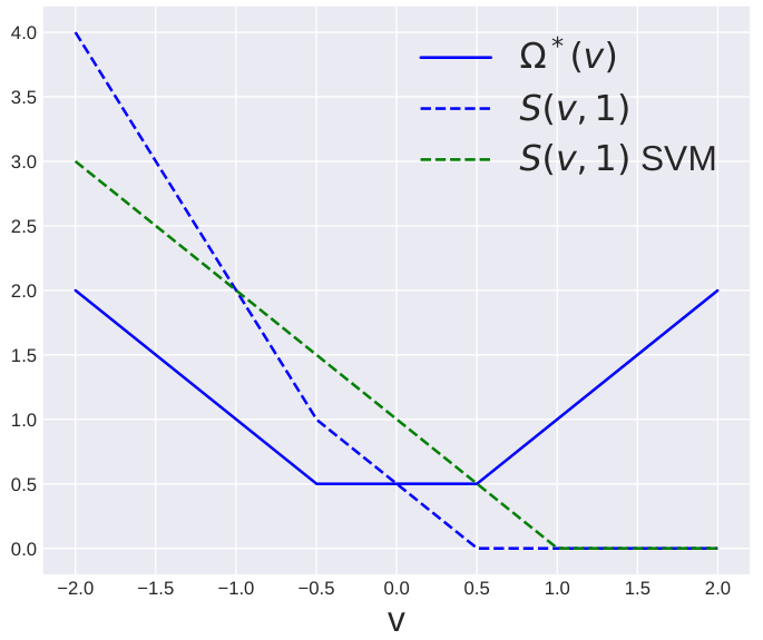
Note that the dependence on yy is only in the linear term v⊤​φ​(y)v^{\top}\varphi(y), while for SSVMs (9) it appears in the maximization. Thus, we can study the geometry of the loss through the non-smooth convex function Ω∗​(v)\Omega^{*}(v) (see fig. 1 for visualizations of some representative unstructured examples). Connections between surrogates (10) and (9) are discussed in section 4.

3.1 Fisher Consistency

Fisher consistency is provided by the following theorem 3.2.

Theorem 3.2 (Fisher Consistency (i)).

The surrogate loss (10) satisfies (i) for g⋆​(x)=−A⊤​φ​(f⋆​(x))g^{\star}(x)=-A^{\top}\varphi(f^{\star}(x)).

This result has been proven by Fathony et al. 2018a in the cost-sensitive multi-class case. Our proof of theorem 3.2 is constructive and based on Fenchel duality.

Sketch of the proof.

We want to show that −A⊤​φ​(f⋆​(x))-A^{\top}\varphi(f^{\star}(x)) is the minimizer of 𝔼y∼ρ(⋅|x)S(v,y)\operatorname{\mathbb{E}}_{y\sim\rho(\cdot|x)}~S(v,y) almost surely for every xx. The proof is constructive and based on Fenchel duality, using the Fenchel-Young loss representation of the max-min surrogate. First, note that the conditional surrogate risk can be written as 𝔼y∼ρ(⋅|x)S(v,y)=Ω∗(v)−v⊤μ(x)\operatorname{\mathbb{E}}_{y\sim\rho(\cdot|x)}~S(v,y)=\Omega^{*}(v)-v^{\top}\mu(x), where μ(x)=𝔼y∼ρ(⋅|x)φ(y)∈ℳ\mu(x)=\operatorname{\mathbb{E}}_{y\sim\rho(\cdot|x)}\varphi(y)\in\mathcal{M}. Second, note that by Fenchel-duality, ∂μΩ⁡(μ⁡(x))\partial_{\mu}\Omega(\mu(x)) is the set of minimizers of Ω∗​(v)−v⊤​μ​(x)\Omega^{*}(v)-v^{\top}\mu(x). Finally, if we assume that the set of x∈𝒳x\in\mathcal{X} such that μ⁡(x)\mu(x) is in the boundary of ℳ\mathcal{M} has measure zero, then

−A⊤​f⋆​(x)∈∂μΩ⁡(μ⁡(x)),-A^{\top}f^{\star}(x)\in\partial_{\mu}\Omega(\mu(x)),

where Ω\Omega is defined in (11) and we have used that f⋆​(x)f^{\star}(x) is the minimizer in yy of φ​(y)⊤​A​μ​(x)\varphi(y)^{\top}A\mu(x). A more detailed proof can be found in section C.1. ∎
Refer to caption
Figure 1: Left: The binary max-min loss has two symmetric kinks instead of one as the SVM. Middle: Ω∗​(v)\Omega^{*}(v) in v⊤​1=0v^{\top}1=0 for multi-class 0-1 loss 1​(y≠y′)1(y\neq y^{\prime}) with k=3k=3. Right: Ω∗​(v)\Omega^{*}(v) in v⊤​1=0v^{\top}1=0 for ordinal regression with the absolute loss |y−y′||y-y^{\prime}| with k=3k=3.

3.2 Comparison Inequality

Fisher consistency is not enough to prove finite-sample generalization bounds on the excess risk ℰ⁡(d∘g)−ℰ⁡(f⋆)\mathcal{E}(d\circ g)-\mathcal{E}(f^{\star}). For this, we provide in the following theorem 3.3 an explicit form of the comparison inequality.

Theorem 3.3 (Comparison inequality (ii)).

Assume LL is symmetric and that there exists C>0C>0 such that for any probability α∈Δ𝒴\alpha\in\Delta_{\mathcal{Y}}, it holds that αy≥1/C\alpha_{y}\geq 1/C for y∈arg​miny∈𝒴⁡𝔼z∼α​L​(y,z)y\in\operatorname*{arg\;min}_{y\in\mathcal{Y}}\mathbb{E}_{z\sim\alpha}L(y,z). Then, the comparison inequality (ii) for the max-min loss (10) reads

ℰ⁡(d∘g)−ℰ⁡(f⋆)≤C⁡(ℛ⁡(g)−ℛ⁡(g⋆)).\mathcal{E}(d\circ g)-\mathcal{E}(f^{\star})\leq C(\mathcal{R}(g)-\mathcal{R}(g^{\star})).

The second condition on the loss states that if yy is optimal for xx, then its conditional probability is bounded away from zero as ρ⁡(y|x)≥1/C\rho(y|x)\geq 1/C. This condition is used to obtain a simple quantitative lower bound on the function ζ\zeta of (ii) and more tight (albeit less explicit in general) expressions of the constant CC can be found in Appendices C.3 and C.4.

Constant 𝑪\boldsymbol{C} for multi-class.

When L⁡(y,y′)=1​(y≠y′)L(y,y^{\prime})=1(y\neq y^{\prime}) with 𝒴={1,…,k}\mathcal{Y}=\{1,\ldots,k\}, we have that C=kC=k, as the minimum conditional probability of an optimal output is 1/k1/k. The constant for this specific setting was derived independently using a different analysis by Duchi et al. 2018.

Constant 𝑪\boldsymbol{C} for factor graphs (example 2.1).

For a factor graph with separable embeddings and a decomposable loss L=1M​∑m=1MLm​(ym,ym′)L=\frac{1}{M}\sum_{m=1}^{M}L_{m}(y_{m},y_{m}^{\prime}), we have that C=maxm∈[M]⁡CmC=\max_{m\in[M]}C_{m}, where CmC_{m} is the constant associated to the individual loss LmL_{m}. This is proven in proposition C.11.

Constant 𝑪\boldsymbol{C} for ranking and matching (example 2.2).

In this setting, theorem 3.3 gives C=M!C=M!, and so the relation between both excess risks is not informative. The problem of exponential constants in the comparison inequality was pointed out by Osokin et al. 2017. We can weaken the assumption and change condition αy≥1/C\alpha_{y}\geq 1/C to

maxβ∈Δ𝒴⁡βy​s.t.​𝔼z∼β⁡φ⁡(z)=𝔼z′∼α⁡φ⁡(z′)≥1/C.\max_{\beta\in\Delta_{\mathcal{Y}}}\beta_{y}\hskip 5.69046pt\text{s.t.}\hskip 5.69046pt\operatorname{\mathbb{E}}_{z\sim\beta}\varphi(z)=\operatorname{\mathbb{E}}_{z^{\prime}\sim\alpha}\varphi(z^{\prime})\geq 1/C.

Under this assumption, we have that C=MC=M, thus avoiding the exponentially large size of the output space.

3.3 Generalization of Regularized ERM

In the following theorem 3.4, we use this result to prove a finite-sample generalization bound on the regularized ERM estimator (3) when the hypothesis space 𝒢\mathcal{G} is a vector-valued RKHS.

Theorem 3.4 (Generalization of regularized ERM).

Let 𝒢\mathcal{G} be a vector-valued RKHS, assume g⋆∈𝒢g^{\star}\in\mathcal{G} and let gng_{n} and λn=κLlog1/2(1/δ)n−1/2\lambda_{n}=\kappa L\log^{1/2}(1/\delta)n^{-1/2} as in (3). Then, with probability 1−δ1-\delta:

ℰ⁡(d∘gn)−ℰ⁡(f⋆)≤M​‖φ⁡(f⋆)‖𝒢​log⁡(1/δ)n,\mathcal{E}(d\circ g_{n})-\mathcal{E}(f^{\star})\leq M\|\varphi(f^{\star})\|_{\mathcal{G}}\sqrt{\frac{\log(1/\delta)}{n}},

with M=κ​C​L​‖A‖M=\kappa CL\|A\|. Here, L=2​maxy∈𝒴​‖φ⁡(y)‖2L=2\max_{y\in\mathcal{Y}}\|\varphi(y)\|_{2}, ‖A‖=sup‖v‖2≤1‖A​v‖2\|A\|=\sup_{\|v\|_{2}\leq 1}\|Av\|_{2}, κ=supx∈𝒳Tr⁡K​(x,x)1/2\kappa=\sup_{x\in\mathcal{X}}\operatorname{Tr}K(x,x)^{1/2} is the size of the features and CC is the one of theorem 3.3.

Analogously to the binary case, the multivariate function φ⁡(f⋆)\varphi(f^{\star}) is piecewise constant on the support of the distribution ρ\rho. In Theorem D.2 in Appendix D we prove that standard low noise conditions, analogous to the one discussed by Pillaud-Vivien et al. 2018b for the binary case, are enough to guarantee ‖φ⁡(f⋆)‖𝒢<∞\|\varphi(f^{\star})\|_{\mathcal{G}}<\infty.

4 Comparison with Structural SVM

Max-min as a correction of the Structural SVM.

We can re-write the maximization over the discrete output space 𝒴\mathcal{Y} in the definition of the SSVM (9) as a maximization over its convex hull ℳ=hull⁡(φ⁡(𝒴))\mathcal{M}=\operatorname{hull}(\varphi(\mathcal{Y}))

S⁡(v,y)=maxμ∈ℳ⁡φ​(y)⊤​A​μ+v⊤​μ−v⊤​φ​(y).\textstyle{S(v,y)=\max_{\mu\in\mathcal{M}}~\varphi(y)^{\top}A\mu+v^{\top}\mu-v^{\top}\varphi(y)}. (12)

Note the similarity between (10) and (12). In particular, the max-min loss differs from the structural SVM in that the maximization is done using miny′∈𝒴⁡φ​(y′)⊤​A​μ\min_{y^{\prime}\in\mathcal{Y}}\varphi(y^{\prime})^{\top}A\mu and not the loss at the observed output yy as φ​(y)⊤​A​μ\varphi(y)^{\top}A\mu. Hence, we can view the max-min surrogate as a correction of the SSVM so that basic statistical properties (i) and (ii) hold. Moreover, this connection might be used to properly understand the statistical properties of SSVM. This is left for future work.

Notion of max-min margin.

Given v∈ℝkv\in\mathbb{R}^{k} and yi∈𝒴y_{i}\in\mathcal{Y}, the classical SSVM is motivated by a soft version of the following notion of margin:

v⊤​φ​(yi)−v⊤​φ​(y)≥L⁡(yi,y)=φ​(yi)⊤​A​φ​(y),v^{\top}\varphi(y_{i})-v^{\top}\varphi(y)\geq L(y_{i},y)=\varphi(y_{i})^{\top}A\varphi(y),

for all y∈𝒴y\in\mathcal{Y}, which is equivalent to v⊤​φ​(yi)−v⊤​μ≥φ​(yi)⊤​A​μv^{\top}\varphi(y_{i})-v^{\top}\mu\geq\varphi(y_{i})^{\top}A\mu for all μ∈ℳ\mu\in\mathcal{M}. However, we have seen in proposition 2.3 that this condition is too strong and only leads to a consistent method if the problem is nearly deterministic, i.e., we observe the optimal yy with large probability, which, as already mentioned, is generally far from true in structured prediction. The max-min surrogate (10) deals with the case where this strong condition is not met and works with a notion of margin that compares groups of outputs instead of just pairs. We define the max-min margin as

v⊤​φ​(yi)−v⊤​μ≥miny′∈𝒴⁡φ​(y′)⊤​A​μ,\textstyle{v^{\top}\varphi(y_{i})-v^{\top}\mu\geq\min_{y^{\prime}\in\mathcal{Y}}\varphi(y^{\prime})^{\top}A\mu,} (13)

for all μ∈ℳ\mu\in\mathcal{M}. After introducing slack variables in (13) we obtain a soft version of the max-min margin that leads to the max-min regularized ERM problem (3).

5 Algorithm

Algorithm 1 GBCFW (primal)
 Let w(0)   .  .  =wi(0)   .  .  =0w^{(0)}\mathrel{\vbox{\hbox{\scriptsize.}\hbox{\scriptsize.}}}=w_{i}^{(0)}\mathrel{\vbox{\hbox{\scriptsize.}\hbox{\scriptsize.}}}=0
 for t=0t=0 to TT do
  Pick ii at random in {1,…,n}\{1,\ldots,n\}
  (μi⋆,νi⋆)∈𝒪K​(gw(t)​(xi),μi⋆,νi⋆)(\mu_{i}^{\star},\nu_{i}^{\star})\in\mathcal{O}_{K}(g_{w^{(t)}}(x_{i}),\mu_{i}^{\star},\nu_{i}^{\star})
  ws   .  .  =Φ⁡(xi)​(μi⋆−φ⁡(yi))⊤/(λ​n)w_{s}\mathrel{\vbox{\hbox{\scriptsize.}\hbox{\scriptsize.}}}=\Phi(x_{i})(\mu_{i}^{\star}-\varphi(y_{i}))^{\top}/(\lambda n)
  wi(t+1)   .  .  =(1−2​nt+2​n)​wi(t)+2​nt+2​n​wsw_{i}^{(t+1)}\mathrel{\vbox{\hbox{\scriptsize.}\hbox{\scriptsize.}}}=(1-\frac{2n}{t+2n})w_{i}^{(t)}+\frac{2n}{t+2n}w_{s}
  w(t+1)   .  .  =w(t)+wi(t+1)−wi(t)w^{(t+1)}\mathrel{\vbox{\hbox{\scriptsize.}\hbox{\scriptsize.}}}=w^{(t)}+w_{i}^{(t+1)}-w_{i}^{(t)}
 end for
Algorithm 2 SP-MP  (μ¯(K),ν¯(K))∈𝒪K​(v,μ(0)​ν(0))(\bar{\mu}^{(K)},\bar{\nu}^{(K)})\in\mathcal{O}_{K}(v,\mu^{(0)}\nu^{(0)})
 for k=0k=0 to K−1K-1 do
  μ1/2(k+1)∈arg​minμ∈ℳ−η​μ⊤​(A⊤​ν(k)+v)+D−H​(μ,μ(k))\mu_{1/2}^{(k+1)}\in{\operatorname*{arg\;min}_{\mu\in\mathcal{M}}}-\eta\mu^{\top}(A^{\top}\nu^{(k)}+v)+D_{-H}(\mu,\mu^{(k)})
  ν1/2(k+1)∈arg​minν∈ℳ⁡η​ν⊤​A​μ(k)+D−H​(ν,ν(k))\nu_{1/2}^{(k+1)}\in{\operatorname*{arg\;min}_{\nu\in\mathcal{M}}}~\eta\nu^{\top}A\mu^{(k)}+D_{-H}(\nu,\nu^{(k)})
  μ(k+1)∈arg​minμ∈ℳ−η​μ⊤​(A⊤​ν1/2(k+1)+v)+D−H​(μ,μ(k))\mu^{(k+1)}\in{\operatorname*{arg\;min}_{\mu\in\mathcal{M}}}-\eta\mu^{\top}(A^{\top}\nu_{1/2}^{(k+1)}+v)+D_{-H}(\mu,\mu^{(k)})
  ν(k+1)∈arg​minν∈ℳ⁡η​ν⊤​A​μ1/2(k+1)+D−H​(ν,ν(k))\nu^{(k+1)}\in{\operatorname*{arg\;min}_{\nu\in\mathcal{M}}}~\eta\nu^{\top}A\mu_{1/2}^{(k+1)}+D_{-H}(\nu,\nu^{(k)})
 end for
 μ¯(K)   .  .  =1K​∑k=1Kμ(k)\textstyle{\bar{\mu}^{(K)}\mathrel{\vbox{\hbox{\scriptsize.}\hbox{\scriptsize.}}}=\frac{1}{K}\sum_{k=1}^{K}\mu^{(k)}}, ν¯(K)   .  .  =1K​∑k=1Kν(k)\textstyle{\bar{\nu}^{(K)}\mathrel{\vbox{\hbox{\scriptsize.}\hbox{\scriptsize.}}}=\frac{1}{K}\sum_{k=1}^{K}\nu^{(k)}}

In this section we derive a dual-based algorithm to solve the max-min regularized ERM problem (3) when the hypothesis space is a RKHS. The algorithm can be easily adapted to the case where gg is parametrized using a neural network as commented at the end of section 5.3.

5.1 Problem Formulation

Let 𝒢⊂{g:𝒳→ℝk}\mathcal{G}\subset\{g:\mathcal{X}\rightarrow\mathbb{R}^{k}\} be a vector-valued RKHS, which we assume of the form 𝒢=ℝk⊗𝒢¯\mathcal{G}=\mathbb{R}^{k}\otimes\overline{\mathcal{G}}, where 𝒢¯\overline{\mathcal{G}} is a scalar RKHS with associated features Φ:𝒳→𝒢¯\Phi:\mathcal{X}\rightarrow\overline{\mathcal{G}}. Every function in 𝒢\mathcal{G} can be written as gw​(x)=w⊤​Φ​(x)∈ℝkg_{w}(x)=w^{\top}\Phi(x)\in\mathbb{R}^{k} where wj,Φ⁡(x)∈𝒢¯w_{j},\Phi(x)\in\overline{\mathcal{G}}. For the sake of presentation, we assume that 𝒢=ℝd×k\mathcal{G}=\mathbb{R}^{d\times k} is finite dimensional, but our analysis also holds for the infinite dimensional case. The dual (D) of the regularized ERM problem (3) for the max-min surrogate loss (10) reads

(D)   maxμ∈ℳn⁡1n​∑i=1nminy′⁡φ​(y′)⊤​A​μi−λ2​‖Φn​(μ−φn)‖22,\displaystyle\max_{\mu\in\mathcal{M}^{n}}~\frac{1}{n}\sum_{i=1}^{n}\min_{y^{\prime}}\varphi(y^{\prime})^{\top}A\mu_{i}-\frac{\lambda}{2}\|\Phi_{n}(\mu-\varphi_{n})\|_{2}^{2},

where Φn=1λ​n​(Φ⁡(x1),…,Φ⁡(xn))\Phi_{n}=\frac{1}{\lambda n}(\Phi(x_{1}),\ldots,\Phi(x_{n})) is the d×nd\times n scaled input data matrix and φn=(φ⁡(y1),…,φ⁡(yn))⊤\varphi_{n}=(\varphi(y_{1}),\ldots,\varphi(y_{n}))^{\top} is the n×kn\times k output data matrix. The dual variables map to the primal variables through the mapping w⁡(μ)=1λ​n​∑i=1nΦ⁡(xi)​(μi−φ⁡(yi))⊤w(\mu)=\frac{1}{\lambda n}\sum_{i=1}^{n}\Phi(x_{i})(\mu_{i}-\varphi(y_{i}))^{\top}. By strong duality, it holds w⋆=w⁡(μ⋆)w^{\star}=w(\mu^{\star}). The dual formulation (D) is a constrained non-smooth optimization problem, where the non-smoothness comes from the first term of the objective function. In order to derive a learning algorithm, we leverage ideas from the block-coordinate Frank-Wolfe algorithm used for SSVMs.

5.2 Derivation of the Algorithm

Background on BCFW for 𝐌𝟑​𝐍𝐬\boldsymbol{\operatorname{M^{3}Ns}}.

The dual of the SSVM is the same as problem (D) but the first term is linear: 1n​∑i=1nφ​(yi)⊤​A​μi\frac{1}{n}\sum_{i=1}^{n}\varphi(y_{i})^{\top}A\mu_{i}, making the dual objective function smooth. The BCFW algorithm (Lacoste-Julien et al. 2013) minimizes a linearization of the smooth dual objective function block-wise, using the separability of the compact domain. At each iteration tt, the algorithm picks i∈[n]i\in[n] at random, and updates μi(t+1)=(1−γ)​μi(t)+γ​μ¯i(t+1)\mu_{i}^{(t+1)}=(1-\gamma)\mu_{i}^{(t)}+\gamma\bar{\mu}_{i}^{(t+1)} with μ¯i(t+1)   .  .  =arg​maxμi′∈ℳ⁡⟨μi′,∇(i)h​(μ(t))⟩\bar{\mu}_{i}^{(t+1)}\mathrel{\vbox{\hbox{\scriptsize.}\hbox{\scriptsize.}}}=\operatorname*{arg\;max}_{\mu_{i}^{\prime}\in\mathcal{M}}~\langle\mu_{i}^{\prime},\nabla_{(i)}h(\mu^{(t)})\rangle where hh is the dual objective and γ\gamma is the step-size. Note that μ¯i(t+1)\bar{\mu}_{i}^{(t+1)} is an extreme point of ℳ\mathcal{M} and it can be written as a combinatorial maximization problem over 𝒴\mathcal{Y} that corresponds precisely to inference (4). In the next subsection, we generalize BCFW to the case where the dual is a sum of a non-smooth and a smooth function such as the dual (D) of our problem.

Generalized BCFW (GBCFW) for 𝐌𝟒​𝐍\boldsymbol{\operatorname{M^{4}N}}.

Borrowing ideas from Bach 2015 in the non block-separable case, we only linearize the smooth-part of the function, i.e., the quadratic term. We change the computation of the direction to

μ¯i(t+1)\displaystyle\bar{\mu}_{i}^{(t+1)}   .  .  =arg​maxμi′∈ℳ⟨μi′,∇(i)−λ2∥Φn(μ(t)−φn)∥22⟩\displaystyle\mathrel{\vbox{\hbox{\scriptsize.}\hbox{\scriptsize.}}}=\operatorname*{arg\;max}_{\mu_{i}^{\prime}\in\mathcal{M}}\langle\mu_{i}^{\prime},\nabla_{(i)}\frac{-\lambda}{2}\|\Phi_{n}(\mu^{(t)}-\varphi_{n})\|_{2}^{2}\rangle
+miny′⁡φ​(y′)⊤​A​μi′=𝒪⁡(gw⁡(μ(t))​(xi)),\displaystyle+\min_{y^{\prime}}\varphi(y^{\prime})^{\top}A\mu_{i}^{\prime}=\mathcal{O}(g_{w(\mu^{(t)})}(x_{i})),

where the max-min oracle 𝒪:ℝk→ℳ\mathcal{O}:\mathbb{R}^{k}\xrightarrow{}\mathcal{M} is defined as

𝒪⁡(v)=arg​maxμ∈ℳ⁡minν∈ℳ​ν⊤​A​μ+v⊤​μ.\textstyle{\mathcal{O}(v)=\operatorname*{arg\;max}_{\mu\in\mathcal{M}}\min_{\nu\in\mathcal{M}}~\nu^{\top}A\mu+v^{\top}\mu.} (14)

Note that the mapping w⁡(μ)w(\mu) between primal and dual variables is affine. Hence, one can write the update of the primal variables without saving the dual variables as detailed in algorithm 1. The following theorem 5.1 specifies the required number of iterations of algorithm 1 to obtain an ε\varepsilon-optimal solution with an approximate oracle (14).

Theorem 5.1 (Convergence of GBCFW with approximate oracle).

Let ε>0\varepsilon>0. If the approximate oracle provides an answer with error ε/2\varepsilon/2, then the final error of algorithm 1 achieves an expected duality gap of ε\varepsilon when T=O~​(n+2​R2λ​ε​diam⁡(ℳ)2)T=\tilde{O}\big(n+\frac{2R^{2}}{\lambda\varepsilon}\operatorname{diam}(\mathcal{M})^{2}\big), where RR is the maximum norm of the features.

5.3 Computation of the Max-Min Oracle

The max-min oracle (14) corresponds to a concave-convex bilinear saddle-point problem. We use a standard alternating procedure of ascent and descent steps on the variables μ\mu and ν\nu, respectively. Consider a strongly concave differentiable entropy H:𝒞⊃ℳ→ℝH:\mathcal{C}\supset\mathcal{M}\rightarrow\mathbb{R} defined in a convex set 𝒞\mathcal{C} containing ℳ\mathcal{M} such that ∇H​(𝒞)=ℝk\nabla H(\mathcal{C})=\mathbb{R}^{k} and limμ∈∂𝒞‖∇H​(μ)‖=+∞\lim_{\mu\in\partial\mathcal{C}}\|\nabla H(\mu)\|=+\infty, where ∂𝒞\partial\mathcal{C} is the boundary of 𝒞\mathcal{C}. Then, perform Mirror ascent/descent updates using −H-H as the Mirror map. For instance, if u=A⊤​ν+vu=A^{\top}\nu+v is the gradient of (14) w.r.t μ\mu, the update on μ\mu takes the following form:

arg​minμ∈ℳ−η​μ⊤​u+D−H​(μ,μ(t)),\textstyle{\operatorname*{arg\;min}_{\mu\in\mathcal{M}}-\eta\mu^{\top}u+D_{-H}(\mu,\mu^{(t)})}, (15)

where D−H(μ,μ′)=−H(μ)+H(μ′)+∇H(μ′)⊤(μ−μ′)D_{-H}(\mu,\mu^{\prime})=-H(\mu)+H(\mu^{\prime})+\nabla H(\mu^{\prime})^{\top}(\mu-\mu^{\prime}) is the Bregman divergence associated to the convex function −H-H. The resulting ascent/descent algorithm has a convergence rate of O(t−1/2)O(t^{-1/2}), which can be considerably improved to O⁡(t−1)O(t^{-1}) with essentially no extra cost by performing four projections instead of two at each iteration. This corresponds to the extra-gradient strategy, called Saddle Point Mirror Prox (SP-MP) when using a Mirror map and is detailed in algorithm 2.

Projection for factor graphs (example 2.1).

The entropy in ℳ\mathcal{M} defined by the factor graph (Wainwright & Jordan 2008) can be written explicitly in terms of the entropies of each part α⊂[M]\alpha\subset[M] if the factor graph has a junction tree structure (Koller & Friedman 2009). For instance, in the case of a sequence of length MM with unary and adjacent pairwise factors, we have H⁡(μ)=∑m=1M−1HS​(μm,m+1)−∑m=1MHS​(μm)\textstyle{H(\mu)=\sum_{m=1}^{M-1}H_{S}(\mu_{m,m+1})-\sum_{m=1}^{M}H_{S}(\mu_{m})}, where HSH_{S} is the Shannon entropy and μm,μm,m+1\mu_{m},\mu_{m,m+1} are the unary and pair-wise marginals, respectively. The projection (15) corresponds to marginal inference in CRFs and can be computed using the sum-product algorithm in time O⁡(M​R2)O(MR^{2}). In this case, the complexity of the projection-oracle is the same the one of the max-oracle for SSVMs.

Projection for ranking and matching (example 2.2).

In this setting, the projection using the entropy in ℳ\mathcal{M} is known to be #P-complete (Valiant 1979). Thus, CRFs are essentially intractable in this setting (Petterson et al. 2009). If instead we use the entropy H(P)=−∑i,j=1MPi​jlogPi​j\textstyle{H(P)=-\sum_{i,j=1}^{M}P_{ij}\log P_{ij}} defined over the marginals P∈ℳP\in\mathcal{M}, the projection can be computed up to precision δ\delta in O⁡(M2/δ)O(M^{2}/\delta) iterations using the Sinkhorn-Knopp algorithm (Cuturi 2013). This can be potentially much cheaper than the max-oracle of SSVMs, which has a cubic dependence in MM. The projection with respect to the Euclidean norm has similar complexity but implementation is more involved (Blondel et al. 2017).

Warm-starting the oracles.

On the one hand, algorithm 1 is guaranteed to converge as long as the error incurred in the oracle 𝒪\mathcal{O} decreases sublinearly with the number of global iterations as εt∝n/(t+n)\varepsilon_{t}\propto n/(t+n) (see section F.1). On the other hand, algorithm 2 can be naturally warm-started because it is an any-time algorithm as the step-size η\eta does not depend on the current iteration or a finite horizon. Hence, we are in a setting where a warm-start strategy can be advantageous. More specifically, at every iteration tt, we save the pairs (μi⋆,νi⋆)∈𝒪⁡(gw(t)​(xi))(\mu_{i}^{\star},\nu_{i}^{\star})\in\mathcal{O}(g_{w^{(t)}}(x_{i})) and the next time we revisit the ii-th training example we initialize algorithm 2 with this pair. Even though the formal demonstration of the effectiveness of the strategy is technically hard, we provide a strong experimental argument showing that a constant number of algorithm 2 iterations are enough to match the allowed error εt\varepsilon_{t}.

Using the kernel trick.

An extension to infinite-dimensional RKHS is straightforward to derive as algorithm 1 is dual-based. In this case, the algorithm keeps track of the dual variables μi\mu_{i} for i=1,…,ni=1,\ldots,n.

Connection to stochastic subgradient algorithms.

It is known that (generalized) conditional gradient methods in the dual are formally equivalent to subgradient methods in the primal (Bach 2015). Indeed, note that wsw_{s} in algorithm 1 is a subgradient of the scaled surrogate loss S⁡(gw​(xi),yi)/λ​nS(g_{w}(x_{i}),y_{i})/\lambda n. However, the dual-based analysis we provide in this paper allows us to derive guarantees on the expected duality gap and a line-search strategy, which we leave for future work. Viewing algorithm 1 as a subgradient method is useful when learning the data representation with a neural network. More specifically, both algorithm 1 and algorithm 2 remain essentially unchanged by applying the chain rule in the update of ww.

5.4 Statistical Analysis of the Algorithm

Finally, the following theorem 5.2 shows that the full algorithm without the warm-start strategy achieves the same statistical error as the regularized ERM estimator (3) after at most O⁡(n​n)O(n\sqrt{n}) projections oracle calls.

Theorem 5.2 (Generalization bound of the algorithm).

Assume the setting of theorem 3.4. Let gn,Tg_{n,T} be the TT-th iteration of algorithm 1 applied to problem (3), where each iteration is computed with K=O⁡(n)K=O(\sqrt{n}) iterations of algorithm 2. Then, after T=O⁡(n)T=O(n) iterations, gn,Tg_{n,T} satisfies the bound of theorem 3.4 with probability 1−δ1-\delta.

As we will show in the next section, in practice a constant number of iterations of algorithm 2 are enough when using the warm-start strategy. Hence, the total number of required projection-oracles is O⁡(n)O(n).

6 Experiments

We perform a comparative experimental analysis for different tasks between M4​N\operatorname{M^{4}N}s, M3​N\operatorname{M^{3}N}s and CRF\operatorname{CRF}s optimized with Generalized BCFW + SP-MP (algorithm 1 + algorithm 2), BCFW (Lacoste-Julien et al. 2013) and SDCA (Shalev-Shwartz & Zhang 2013), respectively. All methods are run with our own implementation 22 2 Code in https://github.com/alexnowakvila/maxminloss. We use datasets of the UCI machine learning repository (Asuncion & Newman 2007) for multi-class classification and ordinal regression, the OCR dataset from Taskar et al. 2004 for sequence prediction and the ranking datasets used by Korba et al. 2018. We use 14 random splits of the dataset into 60% for training, 20% for validation and 20% for testing. We choose the regularization parameter λ\lambda in {2−j}j=110\{2^{-j}\}_{j=1}^{10} using the validation set and show the average test loss on the test sets in table 1 of the model with the best λ\lambda. We use a Gaussian kernel and perform 5050 passes on the data and set the number of iterations of algorithm 2 to 2020 and 1010 times the length of the sequence for sequence prediction. The results are in table 1. We perform better than M3​N\operatorname{M^{3}N}s in most of the datasets for multi-class classification, ordinal regression and ranking, while we obtain similar results in the sequence dataset with the three methods.

Effect of warm-start.

We perform an experiment tracking the test loss and the average error in the max-min oracle for different iterations of algorithm 2 with and without warm-starting. The experiments are done in two datasets for ordinal regression and they are shown in Table 2. We observe that both the test loss and average oracle error are lower for the warm-start strategy. Moreover, when warm-starting the final test error barely changes when increasing the iterations past the 50 iteration threshold.

Task Dataset (d,n,k)(d,n,k) M3​N\operatorname{M^{3}N} CRF\operatorname{CRF} M4​N\operatorname{M^{4}N}
MC segment (19, 2310, 7) 6.64% 6.43% 6.09%
iris (4, 150, 3) 3.33% 3.08% 3.33%
wine (13, 178, 3) 2.56% 2.14% 2.35%
vehicle (18, 846, 4) 24.6% 25.1% 24%
satimage (36, 4435, 6) 12.2% 11.5% 11.9%
letter (16, 15000, 26) 14.6% 13.2% 13.5%
mfeat (216, 2000, 10) 3.94% 4.35% 3.96%
ORD wisconsin (32, 193, 5) 1.24 1.26 1.26
stocks (9, 949, 5) 0.167 0.168 0.160
machine (6, 208, 10) 0.634 0.628 0.628
abalone (10, 4176, 10) 0.520 0.526 0.520
auto (7, 391, 10) 0.589 0.621 0.585
(d,n,M)(d,n,M)
SEQ ocr (128, 6877, 26) 16.2% 16.3% 16.2%
RNK glass (9, 214, 6) 17.7% - 17.4%
bodyfat (7, 252, 7) 79.6% - 79.6%
wine (13, 178, 3) 5.06% - 4.34%
vowel (10, 528, 11) 33.7% - 32.2%
vehicle (18, 846, 4) 14.8% - 15.0%
Table 1: Average test losses on the 14 splits for multi-class classification (first), ordinal regression (second), sequence prediction (third) and ranking (forth). We show in percentage the losses for multi-class, sequence prediction and ranking since they are between zero and one. We show in bold the lowest test loss between the direct classifiers M3​N\operatorname{M^{3}N} and M4​N\operatorname{M^{4}N}.
Dataset W-S K=10K=10 K=30K=30 K=50K=50 K=100K=100
machine yes 0.42 / 0.57 0.41 / 0.43 0.41 / 0.22 0.41 / 0.13
no 0.50 / 4.41 0.50 / 2.74 0.44 / 1.25 0.42 / 0.63
auto yes 0.56 / 1.55 0.55 / 1.29 0.51 / 0.81 0.50 / 0.44
no 0.61 / 2.66 0.57 / 1.79 0.53 / 0.89 0.51 / 0.47
Table 2: We show the (final ordinal test loss / average oracle error at the last epoch) for M4​N\operatorname{M^{4}N}s trained with 100100 passes on data with different iterations of algorithm 2 with and without warm-starting.

7 Conclusion

In this paper, we introduced max-min margin Markov networks (M4​N\operatorname{M^{4}N}s), a method for general structured prediction, that has the same algorithmic and theoretical properties as the regular binary SVM, that is, quantitative convergence bounds through a linear comparison inequality, as well as efficient optimization algorithms. Our experiments show its performance on classical structured prediction problems when using RKHS hypothesis spaces. It would be interesting to extend the analysis of the proposed algorithm by rigorously proving the linear dependence in the number of samples when using the warm-start strategy and incorporating a line-search strategy.

Acknowledgements

The authors would like to thank Mathieu Blondel, Martin Arjovsky and Simon Lacoste-Julien for useful discussions. This work was funded in part by the French government under management of Agence Nationale de la Recherche as part of the “Investissements d’avenir” program, reference ANR-19-P3IA-0001 (PRAIRIE 3IA Institute). We also acknowledge support the European Research Council (grant SEQUOIA 724063). ANV received support from ”La Caixa” Foundation.

References

  • Aronszajn (1950) Aronszajn, N. Theory of reproducing kernels. Transactions of the American Mathematical Society, 68(3):337–404, 1950.
  • Arora et al. (1997) Arora, S., Babai, L., Stern, J., and Sweedyk, Z. The hardness of approximate optima in lattices, codes, and systems of linear equations. Journal of Computer and System Sciences, 54(2):317–331, 1997.
  • Asuncion & Newman (2007) Asuncion, A. and Newman, D. UCI machine learning repository, 2007.
  • Audibert & Tsybakov (2007) Audibert, J.-Y. and Tsybakov, A. B. Fast learning rates for plug-in classifiers. The Annals of statistics, 35(2):608–633, 2007.
  • Bach (2015) Bach, F. Duality between subgradient and conditional gradient methods. SIAM Journal on Optimization, 25(1):115–129, 2015.
  • BakIr et al. (2007) BakIr, G., Hofmann, T., Schölkopf, B., Smola, A. J., Taskar, B., and Vishwanathan, S. Predicting Structured Data. MIT press, 2007.
  • Bartlett et al. (2006) Bartlett, P. L., Jordan, M. I., and McAuliffe, J. D. Convexity, classification, and risk bounds. Journal of the American Statistical Association, 101(473):138–156, 2006.
  • Belanger & McCallum (2016) Belanger, D. and McCallum, A. Structured prediction energy networks. In International Conference on Machine Learning, pp. 983–992, 2016.
  • Blondel et al. (2017) Blondel, M., Seguy, V., and Rolet, A. Smooth and sparse optimal transport. arXiv preprint arXiv:1710.06276, 2017.
  • Blondel et al. (2020) Blondel, M., Martins, A. F., and Niculae, V. Learning with fenchel-young losses. Journal of Machine Learning Research, 21(35):1–69, 2020.
  • Burkard et al. (2012) Burkard, R., Dell’Amico, M., and Martello, S. Assignment problems, revised reprint, volume 106. Siam, 2012.
  • Caetano et al. (2009) Caetano, T. S., McAuley, J. J., Cheng, L., Le, Q. V., and Smola, A. J. Learning graph matching. IEEE Transactions on Pattern Analysis and Machine Intelligence, 31(6):1048–1058, 2009.
  • Ciliberto et al. (2016) Ciliberto, C., Rosasco, L., and Rudi, A. A consistent regularization approach for structured prediction. In Advances in Neural Information Processing Systems, pp. 4412–4420, 2016.
  • Ciliberto et al. (2019) Ciliberto, C., Bach, F., and Rudi, A. Localized structured prediction. In Advances in Neural Information Processing Systems, pp. 7299–7309, 2019.
  • Crammer & Singer (2001) Crammer, K. and Singer, Y. On the algorithmic implementation of multiclass kernel-based vector machines. Journal of machine learning research, 2(Dec):265–292, 2001.
  • Cuturi (2013) Cuturi, M. Sinkhorn distances: Lightspeed computation of optimal transport. In Advances in neural information processing systems, pp. 2292–2300, 2013.
  • De Loera et al. (2012) De Loera, J. A., Hemmecke, R., and Köppe, M. Algebraic and geometric ideas in the theory of discrete optimization. SIAM, 2012.
  • Duchi et al. (2008) Duchi, J., Shalev-Shwartz, S., Singer, Y., and Chandra, T. Efficient projections onto the l 1-ball for learning in high dimensions. In Proceedings of the 25th international conference on Machine learning, pp. 272–279, 2008.
  • Duchi et al. (2018) Duchi, J., Khosravi, K., and Ruan, F. Multiclass classification, information, divergence and surrogate risk. The Annals of Statistics, 46(6B):3246–3275, 2018.
  • Fathony et al. (2016) Fathony, R., Liu, A., Asif, K., and Ziebart, B. Adversarial multiclass classification: A risk minimization perspective. In Advances in Neural Information Processing Systems, pp. 559–567, 2016.
  • Fathony et al. (2018a) Fathony, R., Asif, K., Liu, A., Bashiri, M. A., Xing, W., Behpour, S., Zhang, X., and Ziebart, B. D. Consistent robust adversarial prediction for general multiclass classification. arXiv preprint arXiv:1812.07526, 2018a.
  • Fathony et al. (2018b) Fathony, R., Behpour, S., Zhang, X., and Ziebart, B. Efficient and consistent adversarial bipartite matching. In International Conference on Machine Learning, pp. 1457–1466, 2018b.
  • Fathony et al. (2018c) Fathony, R., Rezaei, A., Bashiri, M. A., Zhang, X., and Ziebart, B. Distributionally robust graphical models. In Advances in Neural Information Processing Systems, pp. 8353–8364, 2018c.
  • Finocchiaro et al. (2019) Finocchiaro, J., Frongillo, R., and Waggoner, B. An embedding framework for consistent polyhedral surrogates. arXiv preprint arXiv:1907.07330, 2019.
  • Jaggi (2013) Jaggi, M. Revisiting frank-wolfe: Projection-free sparse convex optimization. In Proceedings of the 30th international conference on machine learning, pp. 427–435, 2013.
  • Joachims (2006) Joachims, T. Training linear SVMs in linear time. In Proceedings of the SIGKDD International Conference on Knowledge Discovery and Data Mining, pp. 217–226. ACM, 2006.
  • Koller & Friedman (2009) Koller, D. and Friedman, N. Probabilistic graphical models: principles and techniques. MIT press, 2009.
  • Korba et al. (2018) Korba, A., Garcia, A., and d’Alché Buc, F. A structured prediction approach for label ranking. In Advances in Neural Information Processing Systems, pp. 8994–9004, 2018.
  • Kuhn (1955) Kuhn, H. W. The hungarian method for the assignment problem. Naval research logistics quarterly, 2(1-2):83–97, 1955.
  • Lacoste-Julien et al. (2013) Lacoste-Julien, S., Jaggi, M., Schmidt, M., and Pletscher, P. Block-coordinate Frank-Wolfe optimization for structural SVMs. In Proceedings of the 30th International Conference on Machine Learning, pp. 53–61, 2013.
  • Lafferty et al. (2001) Lafferty, J. D., McCallum, A., and Pereira, F. C. N. Conditional random fields: Probabilistic models for segmenting and labeling sequence data. In Proceedings of the Eighteenth International Conference on Machine Learning, 2001.
  • LeCun et al. (2015) LeCun, Y., Bengio, Y., and Hinton, G. Deep learning. nature, 521(7553):436–444, 2015.
  • Lee et al. (2004) Lee, Y., Lin, Y., and Wahba, G. Multicategory support vector machines: Theory and application to the classification of microarray data and satellite radiance data. Journal of the American Statistical Association, 99(465):67–81, 2004.
  • Liu (2007) Liu, Y. Fisher consistency of multicategory support vector machines. In Artificial Intelligence and Statistics, pp. 291–298, 2007.
  • Michelot (1986) Michelot, C. A finite algorithm for finding the projection of a point onto the canonical simplex of n. Journal of Optimization Theory and Applications, 50(1):195–200, 1986.
  • Mroueh et al. (2012) Mroueh, Y., Poggio, T., Rosasco, L., and Slotine, J.-J. Multiclass learning with simplex coding. In Advances in Neural Information Processing Systems, pp. 2789–2797, 2012.
  • Nemirovski (2004) Nemirovski, A. Prox-method with rate of convergence O⁡(1/t){O}(1/t) for variational inequalities with Lipschitz continuous monotone operators and smooth convex-concave saddle point problems. SIAM Journal on Optimization, 15(1):229–251, 2004.
  • Nowak-Vila et al. (2019a) Nowak-Vila, A., Bach, F., and Rudi, A. A general theory for structured prediction with smooth convex surrogates. arXiv preprint arXiv:1902.01958, 2019a.
  • Nowak-Vila et al. (2019b) Nowak-Vila, A., Bach, F., and Rudi, A. Sharp analysis of learning with discrete losses. In The 22nd International Conference on Artificial Intelligence and Statistics, pp. 1920–1929, 2019b.
  • Nowozin & Lampert (2011) Nowozin, S. and Lampert, C. H. Structured learning and prediction in computer vision. Foundations and Trends® in Computer Graphics and Vision, 6(3–4):185–365, 2011.
  • Osokin et al. (2017) Osokin, A., Bach, F., and Lacoste-Julien, S. On structured prediction theory with calibrated convex surrogate losses. In Advances in Neural Information Processing Systems, pp. 302–313, 2017.
  • Petterson et al. (2009) Petterson, J., Yu, J., McAuley, J. J., and Caetano, T. S. Exponential family graph matching and ranking. In Advances in Neural Information Processing Systems, pp. 1455–1463, 2009.
  • Pillaud-Vivien et al. (2018a) Pillaud-Vivien, L., Rudi, A., and Bach, F. Exponential convergence of testing error for stochastic gradient methods. Proceedings of the Conference on Learning Theory, 2018a.
  • Pillaud-Vivien et al. (2018b) Pillaud-Vivien, L., Rudi, A., and Bach, F. Exponential convergence of testing error for stochastic gradient methods. In Proceedings of the Conference On Learning Theory, pp. 250–296, 2018b.
  • Ramaswamy & Agarwal (2016) Ramaswamy, H. G. and Agarwal, S. Convex calibration dimension for multiclass loss matrices. Journal of Machine Learning Research, 17(1):397–441, 2016.
  • Ramaswamy et al. (2013) Ramaswamy, H. G., Agarwal, S., and Tewari, A. Convex calibrated surrogates for low-rank loss matrices with applications to subset ranking losses. In Advances in Neural Information Processing Systems, pp. 1475–1483, 2013.
  • Ryser (1963) Ryser, H. J. Combinatorial mathematics, volume 14. American Mathematical Soc., 1963.
  • Shalev-Shwartz & Zhang (2013) Shalev-Shwartz, S. and Zhang, T. Stochastic dual coordinate ascent methods for regularized loss minimization. Journal of Machine Learning Research, 14(Feb):567–599, 2013.
  • Smith (2011) Smith, N. A. Linguistic structure prediction. Synthesis lectures on human language technologies, 4(2):1–274, 2011.
  • Sridharan et al. (2009) Sridharan, K., Shalev-Shwartz, S., and Srebro, N. Fast rates for regularized objectives. In Advances in Neural Information Processing Systems, pp. 1545–1552, 2009.
  • Taskar et al. (2004) Taskar, B., Guestrin, C., and Koller, D. Max-margin Markov networks. In Advances in neural information processing systems, pp. 25–32, 2004.
  • Taskar et al. (2005) Taskar, B., Chatalbashev, V., Koller, D., and Guestrin, C. Learning structured prediction models: A large margin approach. In Proceedings of the 22nd international conference on Machine learning, pp. 896–903, 2005.
  • Tsochantaridis et al. (2005) Tsochantaridis, I., Joachims, T., Hofmann, T., and Altun, Y. Large margin methods for structured and interdependent output variables. Journal of machine learning research, 6(Sep):1453–1484, 2005.
  • Valiant (1979) Valiant, L. G. The complexity of computing the permanent. Theoretical computer science, 8(2):189–201, 1979.
  • Viterbi (1967) Viterbi, A. Error bounds for convolutional codes and an asymptotically optimum decoding algorithm. IEEE transactions on Information Theory, 13(2):260–269, 1967.
  • Wainwright & Jordan (2008) Wainwright, M. J. and Jordan, M. I. Graphical models, exponential families, and variational inference. Foundations and Trends® in Machine Learning, 1(1–2):1–305, 2008.
  • Zhang (2004) Zhang, T. Statistical analysis of some multi-category large margin classification methods. Journal of Machine Learning Research, 5(Oct):1225–1251, 2004.

Organization of the Appendix

  • A.

    Notation

  • B.

    Geometrical Properties

    • B.1.

      Geometry of the loss L

    • B.2.

      Geometry of the loss S

    • B.3.

      Relation between cell complexes

    • B.4.

      Examples

  • C.

    Theoretical properties of the Surrogate

    • C.1.

      Fisher consistency
      Here Theorem 3.2 is derived as Theorem C.3.

    • C.2.

      Comparison inequality and calibration function

    • C.3.

      Characterizing the calibration function for Max-Min Markov Networks

    • C.4.

      Quantitative lower bound
      Here Theorem 3.3 is derived as Theorem C.8.

    • C.5.

      Computation of the constant for specific losses

  • D.

    Sharp Generalization Bounds for Regularized Objectives
    Here Theorem 3.4 is derived.

  • E.

    Max-min margin and dual formulation

    • E.1

      Derivation of the Dual Formulation

    • E.2

      Computation of the Dual Gap

  • F.

    Generalized Block-Coordinate Frank-Wolfe

    • F.1.

      General Convergence Result

    • F.2.

      Application to 𝐌𝟒​𝐍\boldsymbol{\operatorname{M^{4}N}}
      Here Theorem 5.1 is proven using the analysis from section F.1.

  • G.

    Solving the Oracle with Saddle Point Mirror Prox

    • G.1.

      Saddle Point Mirror Prox (SP-MP

    • G.2.

      Max-Min Oracle for Sequences

    • G.3.

      Max-Min Oracle for Ranking and Matching

  • H.

    Generalization Bounds for 𝐌𝟒​𝐍\boldsymbol{\operatorname{M^{4}N}} solved via GBCFW and Approximate Oracle
    Here Theorem 5.2 is proven combining the results from section D and Theorem 5.1.

Appendix A Notation

In this section we introduce some notation that will be useful in the rest of the appendix.

Notation on the structured prediction setting. Denote by 𝒫⁡(A)\mathcal{P}(A) the set of subsets of the set AA. We define the following quantities

  • -

    Marginal polytope: ℳ=hull(φ(𝒴))={v∈ℝk|v=∑y∈𝒴αyφ(y),α∈Δ𝒴}\mathcal{M}=\operatorname{hull}(\varphi(\mathcal{Y}))=\{v\in\mathbb{R}^{k}~|~v=\sum_{y\in\mathcal{Y}}\alpha_{y}\varphi(y),\alpha\in\Delta_{\mathcal{Y}}\}.

  • -

    Normal cone of ℳ\mathcal{M} at μ\mu: 𝒩ℳ(μ)={u∈ℝk|⟨μ′−μ,u⟩≤0,∀μ′∈ℳ}\mathcal{N}_{\mathcal{M}}(\mu)=\{u\in\mathbb{R}^{k}~|~\langle\mu^{\prime}-\mu,u\rangle\leq 0,\forall\mu^{\prime}\in\mathcal{M}\}.

  • -

    Conditional moments: ν⁡(q)=𝔼y′∼q⁡φ⁡(y′)∈ℳ\nu(q)=\operatorname{\mathbb{E}}_{y^{\prime}\sim q}\varphi(y^{\prime})\in\mathcal{M} where q∈Prob⁡(𝒴)q\in\operatorname{Prob}(\mathcal{Y}).

  • -

    Conditional risk: ℓ⁡(y,μ)   .  .  =𝔼y′∼q⁡L⁡(y,y′)=φ​(y)⊤​A​μ\ell(y,\mu)\mathrel{\vbox{\hbox{\scriptsize.}\hbox{\scriptsize.}}}=\operatorname{\mathbb{E}}_{y^{\prime}\sim q}L(y,y^{\prime})=\varphi(y)^{\top}A\mu.

  • -

    Bayes risk: ℓ⁡(μ)   .  .  =miny∈𝒴⁡ℓ⁡(y,μ)\ell(\mu)\mathrel{\vbox{\hbox{\scriptsize.}\hbox{\scriptsize.}}}=\min_{y\in\mathcal{Y}}\ell(y,\mu)

  • -

    Minus Bayes risk: Ω⁡(μ)   .  .  =−ℓ⁡(μ)+1ℳ​(μ)\Omega(\mu)\mathrel{\vbox{\hbox{\scriptsize.}\hbox{\scriptsize.}}}=-\ell(\mu)+1_{\mathcal{M}}(\mu).

  • -

    Excess conditional risk: δ​ℓ​(y,μ)=ℓ⁡(y,μ)−ℓ⁡(μ)\delta\ell(y,\mu)=\ell(y,\mu)-\ell(\mu)

  • -

    Optimal predictor set: y⋆​(μ)=arg​miny∈𝒴⁡ℓ​(y,μ)⊆𝒴y^{\star}(\mu)=\operatorname*{arg\;min}_{y\in\mathcal{Y}}~\ell(y,\mu)\subseteq\mathcal{Y}.

  • -

    Marginal polytope cell complex: 𝒞⁡(ℳ)=(y⋆)−1∘y⋆​(ℳ)⊂𝒫⁡(ℳ)\mathcal{C}(\mathcal{M})=(y^{\star})^{-1}\circ y^{\star}(\mathcal{M})\subset\mathcal{P}(\mathcal{M}).

Notation on the max-min surrogate.

  • -

    Partition function: Ω∗​(v)=maxμ∈ℳ⁡ℓ⁡(μ)+v⊤​μ\Omega^{*}(v)=\max_{\mu\in\mathcal{M}}\ell(\mu)+v^{\top}\mu.

  • -

    Surrogate loss: S⁡(v,y)=Ω∗​(v)−v⊤​φ​(y)S(v,y)=\Omega^{*}(v)-v^{\top}\varphi(y).

  • -

    Conditional surrogate risk: s⁡(v,μ)   .  .  =𝔼y∼q⁡S⁡(v,y)=Ω∗​(v)−v⊤​μs(v,\mu)\mathrel{\vbox{\hbox{\scriptsize.}\hbox{\scriptsize.}}}=\operatorname{\mathbb{E}}_{y\sim q}S(v,y)=\Omega^{*}(v)-v^{\top}\mu.

  • -

    Bayes surrogate risk: s⁡(μ)   .  .  =minv∈ℝk⁡s⁡(v,μ)(=ℓ⁡(μ))s(\mu)\mathrel{\vbox{\hbox{\scriptsize.}\hbox{\scriptsize.}}}=\min_{v\in\mathbb{R}^{k}}s(v,\mu)\quad(=\ell(\mu)).

  • -

    Excess surrogate conditional risk: δ​s​(v,μ)   .  .  =s⁡(v,μ)−s⁡(μ)\delta s(v,\mu)\mathrel{\vbox{\hbox{\scriptsize.}\hbox{\scriptsize.}}}=s(v,\mu)-s(\mu).

  • -

    Optimal predictors: v⋆​(μ)=arg​minv∈ℝk⁡s​(v,μ)⊂ℝkv^{\star}(\mu)=\operatorname*{arg\;min}_{v\in\mathbb{R}^{k}}~s(v,\mu)\subset\mathbb{R}^{k}.

  • -

    Surrogate space cell complex: 𝒞⁡(ℝk)=v⋆​(ℳ)⊂𝒫⁡(ℝk)\mathcal{C}(\mathbb{R}^{k})=v^{\star}(\mathcal{M})\subset\mathcal{P}(\mathbb{R}^{k}).

Appendix B Geometrical Properties

In this section, we study the rich geometrical properties of the max-min surrogate construction. The geometrical interpretation provides a valuable intuition on different key mathematical objects appearing in the further analysis needed for the proofs of the main theorems. More precisely, we show that the max-min surrogate loss SS defines a partition 𝒞⁡(ℝk)⊂𝒫⁡(ℝk)\mathcal{C}(\mathbb{R}^{k})\subset\mathcal{P}(\mathbb{R}^{k}) of the surrogate space ℝk\mathbb{R}^{k} which is dual to the partition 𝒞⁡(ℳ)⊂𝒫⁡(ℳ)\mathcal{C}(\mathcal{M})\subset\mathcal{P}(\mathcal{M}) of the marginal polytope ℳ\mathcal{M} defined by LL. Moreover, we show that the mapping between those partitions is the subgradient mapping ∂Ω\partial\Omega with inverse ∂Ω∗\partial\Omega^{*} (see fig. 2). Visualization for binary 0-1 loss, multi-class 0-1 loss, absolute loss for ordinal regression and Hamming loss are provided in section B.4.

Figure 2: The cell complex 𝒞⁡(ℳ)\mathcal{C}(\mathcal{M}) on the marginal polytope ℳ\mathcal{M} maps to the cell complex 𝒞⁡(ℝk)\mathcal{C}(\mathbb{R}^{k}) on the surrogate space ℝk\mathbb{R}^{k} through the subgradient mapping of the partition function ∂Ω\partial\Omega.

Following (Finocchiaro et al. 2019), we now introduce the definition of a cell complex.

Definition B.1 (Cell complex).

A cell complex in ℝk\mathbb{R}^{k} is a set 𝒞\mathcal{C} of faces (of dimension 0,…,k0,\ldots,k) such that:

  • (i)

    union to ℝk\mathbb{R}^{k}.

  • (ii)

    have pairwise disjoint relative interiors.

  • (iii)

    any nonempty intersection of faces F,F′F,F^{\prime} in 𝒞\mathcal{C} is a face of FF and F′F^{\prime} and an element of 𝒞\mathcal{C}.

Any convex affine-by-parts function has an associated cell complex defined by considering the polytope corresponding to the epigraph of the function and projecting the faces down to to the domain. Moreover, if f⁡(v)f(v) is convex affine-by-parts, the cell complex associated to f⁡(v)f(v) and f⁡(v)+v⊤​af(v)+v^{\top}a are the same for any aa.

B.1 Geometry of the Loss L

The convex affine-by-parts function Ω⁡(μ)=−ℓ⁡(μ)+1ℳ​(μ)\Omega(\mu)=-\ell(\mu)+1_{\mathcal{M}}(\mu) naturally defines a cell complex of its domain ℳ\mathcal{M} (see for instance (Ramaswamy & Agarwal 2016; Nowak-Vila et al. 2019a)). This can be constructed by considering the polyhedra corresponding to the epigraph of −ℓ⁡(μ)-\ell(\mu) and then projecting the faces to ℳ\mathcal{M}. Each face corresponds to a different group of active hyperplanes in the definition of ℓ⁡(μ)\ell(\mu). The cell complex can be defined as 𝒞⁡(ℳ)={(y⋆)−1∘y⋆​(μ)¯|μ∈ℳ}⊂𝒫⁡(ℳ)\mathcal{C}(\mathcal{M})=\{\overline{(y^{\star})^{-1}\circ y^{\star}(\mu)}~|~\mu\in\mathcal{M}\}\subset\mathcal{P}(\mathcal{M}), i.e., each face is defined as the set of moments that share the same set of optimal predictors. Note that 𝒞⁡(ℳ)\mathcal{C}(\mathcal{M}) contains faces of 0-dimensions (points) up to faces of kk-dimensions.

B.2 Geometry of the Loss S

Recall that S⁡(v,y)=Ω∗​(v)−v⊤​μS(v,y)=\Omega^{*}(v)-v^{\top}\mu and Ω⁡(μ)=−ℓ⁡(μ)+1ℳ​(μ)\Omega(\mu)=-\ell(\mu)+1_{\mathcal{M}}(\mu), where ℓ⁡(μ)\ell(\mu) is concave affine-by-parts. In particular, as Ω\Omega is convex affine-by-parts with compact domain, then Ω∗\Omega^{*} is convex affine-by-parts with full-dimensional domain ℝk\mathbb{R}^{k}. The projection of the faces of the convex polyhedron defined as the epigraph of Ω∗\Omega^{*} defines a cell complex 𝒞⁡(ℝk)⊂𝒫⁡(ℝk)\mathcal{C}(\mathbb{R}^{k})\subset\mathcal{P}(\mathbb{R}^{k}) in the (unbounded) vector space ℝk\mathbb{R}^{k}. The cell complex defined by Ω∗​(v)\Omega^{*}(v) is the same as the one defined by s⁡(v,μ)=Ω∗​(v)−v⊤​μs(v,\mu)=\Omega^{*}(v)-v^{\top}\mu for every μ∈ℳ\mu\in\mathcal{M}. The faces of 𝒞⁡(ℝk)\mathcal{C}(\mathbb{R}^{k}) can be written as v⋆​(μ)=arg​minv∈ℝk⁡s​(v,μ)∈𝒫⁡(ℝk)v^{\star}(\mu)=\operatorname*{arg\;min}_{v\in\mathbb{R}^{k}}~s(v,\mu)\in\mathcal{P}(\mathbb{R}^{k}) for a certain μ∈ℳ\mu\in\mathcal{M}, i.e., the faces are the minimizers of the conditional surrogate risk. Hence, we can write in a compact form v⋆​(μ)∈𝒞⁡(ℝk)v^{\star}(\mu)\in\mathcal{C}(\mathbb{R}^{k}).

B.3 Relation between Cell Complexes

Recall that 𝒞⁡(ℳ)\mathcal{C}(\mathcal{M}) is generated by projecting the faces of the epigraph of Ω\Omega while 𝒞⁡(ℝk)\mathcal{C}(\mathbb{R}^{k}) is generated by projecting the faces of the epigraph of Ω∗\Omega^{*}. The subgradients are well-defined in the cell complexes and define a bijection between them:

∂Ω:𝒞⁡(ℳ)→𝒞⁡(ℝk),∂Ω∗:𝒞⁡(ℝk)→𝒞⁡(ℳ),∂Ω∗=(∂Ω)−1.\partial\Omega:\mathcal{C}(\mathcal{M})\rightarrow\mathcal{C}(\mathbb{R}^{k}),\hskip 28.45274pt\partial\Omega^{*}:\mathcal{C}(\mathbb{R}^{k})\rightarrow\mathcal{C}(\mathcal{M}),\hskip 28.45274pt\partial\Omega^{*}=(\partial\Omega)^{-1}.

Moreover, we have that

dim⁡(∂Ω⁡(F))\displaystyle\operatorname{dim}(\partial\Omega(F)) =dim⁡(ℳ)−dim⁡(F),\displaystyle=\operatorname{dim}(\mathcal{M})-\operatorname{dim}(F),\hskip 28.45274pt ∀F∈𝒞⁡(ℳ)\displaystyle\forall F\in\mathcal{C}(\mathcal{M})
dim⁡(∂Ω∗​(F′))\displaystyle\operatorname{dim}(\partial\Omega^{*}(F^{\prime})) =dim⁡(ℳ)−dim⁡(F′),\displaystyle=\operatorname{dim}(\mathcal{M})-\operatorname{dim}(F^{\prime}),\hskip 28.45274pt ∀F′∈𝒞⁡(ℝk),\displaystyle\forall F^{\prime}\in\mathcal{C}(\mathbb{R}^{k}),

where F,F′F,F^{\prime} are faces of 𝒞⁡(ℳ),𝒞⁡(ℝk)\mathcal{C}(\mathcal{M}),\mathcal{C}(\mathbb{R}^{k}), respectively.

B.4 Examples

Let’s now provide some concrete examples of cell complexes and the associated mapping subgradient mapping for several classical tasks.

Binary Classification.

The output space is 𝒴={−1,1}\mathcal{Y}=\{-1,1\}. The loss is L⁡(y,y′)=1​(y≠y′)L(y,y^{\prime})=1(y\neq y^{\prime}) with affine decomposition a=1a=1, φ⁡(1)=(1,0)⊤\varphi(1)=(1,0)^{\top}, φ⁡(−1)=(0,1)⊤\varphi(-1)=(0,1)^{\top} and A=−I2×2A=-I_{2\times 2}. The marginal polytope is ℳ=Δ2\mathcal{M}=\Delta_{2}.

Ω⁡(p)=−min⁡(p,1−p)+1Δ2​(p),Ω∗​(v)=max⁡(|v|,1/2),S⁡(v,y)=Ω∗​(v)−y​v.\Omega(p)=-\min(p,1-p)+1_{\Delta_{2}}(p),\hskip 14.22636pt\Omega^{*}(v)=\max(|v|,1/2),\hskip 14.22636ptS(v,y)=\Omega^{*}(v)-yv.
Figure 3: Binary 0-1 loss. Left: The Bayes risk −Ω-\Omega is a concave polyhedral function defined in Δ2=[0,1]\Delta_{2}=[0,1]. The faces of the induced cell-complex are the 0-dimensional faces {0},{1/2},{1}\{0\},\{1/2\},\{1\} and the 1-dimensional faces [0,1/2][0,1/2], [1/2,1][1/2,1]. Right: The partition function is a convex polyhedral function defined in ℝ\mathbb{R}. The faces of the induced cell-complex are the 0-dimensional faces {−1/2}\{-1/2\}, {1/2}\{1/2\} and the 1-dimensional faces (−∞,−1/2](-\infty,-1/2], [1/2,1/2][1/2,1/2], [1/2,+∞)[1/2,+\infty).

See fig. 3. The mapping between cells is

∂Ω({0})=(−∞,−1/2],∂Ω∗((−∞,−1/2])={0}∂Ω({1/2})=[−1/2,1/2],∂Ω∗([−1/2,1/2])={1/2}∂Ω({1})=[1/2,+∞),∂Ω∗([1/2,+∞))={1}∂Ω([0,1/2])={−1/2},∂Ω∗({−1/2})=[0,1/2]∂Ω⁡([1/2,1])={1/2},∂Ω∗​({1/2})=[1/2,1]\begin{array}[]{lll}&\partial\Omega(\{0\})=(-\infty,-1/2],&\partial\Omega^{*}((-\infty,-1/2])=\{0\}\\ &\partial\Omega(\{1/2\})=[-1/2,1/2],&\partial\Omega^{*}([-1/2,1/2])=\{1/2\}\\ &\partial\Omega(\{1\})=[1/2,+\infty),&\partial\Omega^{*}([1/2,+\infty))=\{1\}\\ &\partial\Omega([0,1/2])=\{-1/2\},&\partial\Omega^{*}(\{-1/2\})=[0,1/2]\\ &\partial\Omega([1/2,1])=\{1/2\},&\partial\Omega^{*}(\{1/2\})=[1/2,1]\\ \end{array}

0-1 Multi-class Classification.

The output space is 𝒴=[k]={1,⋯,k}\mathcal{Y}=[k]=\{1,\cdots,k\}. The loss is L⁡(y,y′)=1​(y≠y′)L(y,y^{\prime})=1(y\neq y^{\prime}) with affine decomposition a=1a=1, φ⁡(y)=ey\varphi(y)=e_{y} and A=−Ik×kA=-I_{k\times k}, where ey∈ℝke_{y}\in\mathbb{R}^{k} is the yy-th vector of the canonical basis in ℝk\mathbb{R}^{k}. The marginal polytope is the kk-dimensional simplex ℳ=Δk\mathcal{M}=\Delta_{k}.

In this case, ℓ⁡(p)=1−‖p‖∞\ell(p)=1-\|p\|_{\infty} and so

Ω⁡(p)=‖p‖∞−1+1Δk​(p),Ω∗​(v)=1+maxj∈[k]⁡{1j​∑r=1jv(r)−1j},\Omega(p)=\|p\|_{\infty}-1+1_{\Delta_{k}}(p),\hskip 14.22636pt\Omega^{*}(v)=1+\max_{j\in[k]}\bigg\{\frac{1}{j}\sum_{r=1}^{j}v_{(r)}-\frac{1}{j}\bigg\},

where v(1)≥⋯≥v(k)v_{(1)}\geq\cdots\geq v_{(k)} (see fig. 4).

Figure 4: Multi-class 0-1 loss (k=3k=3). Left: The Bayes risk −Ω-\Omega has a pyramid shape centered at the simplex. The cell-complex 𝒞⁡(Δk)\mathcal{C}(\Delta_{k}) has 2k2^{k} 0-dimensional faces (points) and kk full-dimensional faces. In the figure, the set of points are the center point, the 3 vertices of the triangle and the 3 middle points in the triangle face. The 3 full-dimensional faces are the 3 colored zones. Right: The partition function Ω∗\Omega^{*} is a convex polyhedral function. The cell-complex has kk 0-dimensional faces (points) and 2k2^{k} full-dimensional faces. In the figure, the set of points are the 3 vertices of the triangle in the center and the full-dimensional faces are the colored zones.

Note that the subgradient mapping ∂Ω\partial\Omega sends the 2k2^{k} 0-dimensional faces (points) and the full-dimensional faces of 𝒞⁡(Δk)\mathcal{C}(\Delta_{k}) to the full-dimensional faces and 0-dimensional faces of 𝒞⁡(ℝk−1)\mathcal{C}(\mathbb{R}^{k-1}), respectively.

Ordinal Regression.

The output space is the same as for multiclass classification, but in this case there is an implicit ordering between outputs: 1≺2≺⋯≺k1\prec 2\prec\cdots\prec k. This is encoded using the absolute difference loss L⁡(y,y′)=|y−y′|L(y,y^{\prime})=|y-y^{\prime}|. We consider the affine decomposition φ⁡(y)=ey∈ℝk\varphi(y)=e_{y}\in\mathbb{R}^{k}, A=(|i−j|)i,j∈[k]2A=(|i-j|)_{i,j\in[k]^{2}} and a=0a=0. It is possible to obtain a closed form expression for the partition function (see Thm. 6 by (Fathony et al. 2018a)):

Ω∗​(v)=12​maxi,j∈[k]​vi+vj+j−i.\Omega^{*}(v)=\frac{1}{2}\max_{i,j\in[k]}~v_{i}+v_{j}+j-i.

In fig. 5 we plot the Bayes risk and the partition function for the ordinal loss. Note that that the topology of the cell-complex is different from the previous example.

Figure 5: Absolute difference loss (k=3k=3). Left: The Bayes risk −Ω-\Omega has an asymmetrical pyramid shape with the tip in one face of the simplex. Right: The partition function Ω∗\Omega^{*} has a different topology than the one from multi-class.

Multi-label Classification with Hamming Loss.

This corresponds to example 2.1 with unary potentials. Let 𝒴=Πm=1M​𝒴m\mathcal{Y}=\Pi_{m=1}^{M}\mathcal{Y}_{m} with 𝒴m={1,…,R}\mathcal{Y}_{m}=\{1,\dots,R\}. We consider the Hamming loss defined as an average of multi-class losses: L⁡(y,y′)=1M​∑m=1M1​(ym≠ym′)L(y,y^{\prime})=\frac{1}{M}\sum_{m=1}^{M}1(y_{m}\neq y_{m}^{\prime}). The marginal polytope factorizes as ℳ=Πm=1M​ΔR\mathcal{M}=\Pi_{m=1}^{M}\Delta_{R}. The Bayes risk decomposes additively as the sum of the Bayes risks of the individual multi-class losses and the partition function decomposes analogously. In fig. 6 we plot the Bayes risk and the partition function for R=M=2R=M=2.

Figure 6: Hamming loss for (R=M=2)(R=M=2). Left: The marginal polytope is the cube ℳ=[0,1]2\mathcal{M}=[0,1]^{2} and the Bayes risk −Ω-\Omega has a pyramid shape centered in the cube. Right: The partition function Ω∗\Omega^{*}.

Appendix C Theoretical Properties of the Surrogate

The goal of this section is to prove the two theoretical requirements for the surrogate method. These are Fisher consistency (1) and a comparison inequality (2):

(1)ℰ⁡(f⋆)=ℰ⁡(d∘g⋆)(2)ζ⁡(ℰ⁡(d∘g)−ℰ⁡(f⋆))≤ℛ⁡(g)−ℛ⁡(g⋆).\begin{array}[]{ll}\text{(1)}&\mathcal{E}(f^{\star})=\mathcal{E}(d\circ g^{\star})\\ \text{(2)}&\zeta(\mathcal{E}(d\circ g)-\mathcal{E}(f^{\star}))\leq\mathcal{R}(g)-\mathcal{R}(g^{\star}).\end{array}

for all measurable g:𝒳→ℋg:\mathcal{X}\xrightarrow{}\mathcal{H}, where ζ:ℝ→ℝ\zeta:\mathbb{R}\xrightarrow{}\mathbb{R} is such that ζ⁡(ε)→0\zeta(\varepsilon)\to 0 if ε→0\varepsilon\to 0. Fisher consistency ensures that the optimum of the surrogate loss g⋆g^{\star} provides the Bayes optimum f⋆f^{\star} of the problem. However, in practice the optimum of the surrogate is never attained and so one wants to control how close f=d∘gf=d\circ g is to f⋆f^{\star} in terms of the estimation error of gg to g⋆g^{\star}. The comparison inequality gives this quantification by relating the excess expected risk ℰ⁡(d∘g)−ℰ⁡(f⋆)\mathcal{E}(d\circ g)-\mathcal{E}(f^{\star}) to the excess expected surrogate risk ℛ⁡(g)−ℛ⁡(g⋆)\mathcal{R}(g)-\mathcal{R}(g^{\star}), which allows to translate rates from the surrogate problem to the original problem.

Let’s start first by showing that s⁡(μ)=ℓ⁡(μ)s(\mu)=\ell(\mu) for all μ∈ℳ\mu\in\mathcal{M}, i.e., that the minimizers of the conditional surrogate risks coincide.

Lemma C.1.

The Bayes risk and the surrogate Bayes risk are the same:

s⁡(μ)=minv∈ℝk⁡s⁡(v,μ)=miny′∈𝒴⁡ℓ⁡(y,μ)=ℓ⁡(μ),∀μ∈ℳ.s(\mu)=\min_{v\in\mathbb{R}^{k}}~s(v,\mu)=\min_{y^{\prime}\in\mathcal{Y}}~\ell(y,\mu)=\ell(\mu),\hskip 28.45274pt\forall\mu\in\mathcal{M}.
Proof.

Note that s⁡(μ)=minv∈ℝk⁡s⁡(v,μ)=minv∈ℝk⁡Ω∗​(v)−v⊤​μ=−Ω=ℓ⁡(μ)−1ℳ​(μ)s(\mu)=\min_{v\in\mathbb{R}^{k}}~s(v,\mu)=\min_{v\in\mathbb{R}^{k}}~\Omega^{*}(v)-v^{\top}\mu=-\Omega=\ell(\mu)-1_{\mathcal{M}}(\mu). ∎

Note that this is not the case for smooth surrogates. It was noted by (Finocchiaro et al. 2019) (see Prop. 1 and 2) that consistent polyhedral surrogates necessarily satisfy the property of matching Bayes risks.

C.1 Fisher Consistency

The following proposition C.2 characterizes the form of the exact minimizer of the conditional surrogate risk s⁡(v,μ)s(v,\mu).

Proposition C.2.

Let μ∈ℳ\mu\in\mathcal{M} and y⋆​(μ)=arg​miny∈𝒴⁡φ​(y)⊤​A​μy^{\star}(\mu)=\operatorname*{arg\;min}_{y\in\mathcal{Y}}\varphi(y)^{\top}A\mu be the set of optimal predictors. Then, we have that

hull⁡(−A⊤​φ​(y))y∈y⋆​(μ)+𝒩ℳ​(μ)=arg​minv∈ℝk⁡s​(v,μ).\operatorname{hull}(-A^{\top}\varphi(y))_{y\in y^{\star}(\mu)}+\mathcal{N}_{\mathcal{M}}(\mu)=\operatorname*{arg\;min}_{v\in\mathbb{R}^{k}}s(v,\mu). (16)
Proof.

The proof consists in noticing that hull⁡(−A⊤​φ​(y))y∈y⋆​(μ)\operatorname{hull}(-A^{\top}\varphi(y))_{y\in y^{\star}(\mu)} is a subgradient at μ\mu of the non-smooth convex function Ω=−ℓ⁡(μ)+1ℳ​(μ)\Omega=-\ell(\mu)+1_{\mathcal{M}}(\mu) with compact domain ℳ\mathcal{M}. That is,

Ω⁡(μ)\displaystyle\Omega(\mu) =−miny′∈𝒴⁡φ​(y′)⊤​A​μ+1ℳ​(μ)\displaystyle=-\min_{y^{\prime}\in\mathcal{Y}}\varphi(y^{\prime})^{\top}A\mu+1_{\mathcal{M}}(\mu)
=−φ​(y)⊤​A​μ+1ℳ​(μ),y∈y⋆​(μ).\displaystyle=-\varphi(y)^{\top}A\mu+1_{\mathcal{M}}(\mu),\hskip 28.45274pty\in y^{\star}(\mu).

The subgradient reads ∂Ω⁡(μ)=−hull⁡(A⊤​φ​(y))y∈y⋆​(μ)+𝒩ℳ​(μ)\partial\Omega(\mu)=-\operatorname{hull}(A^{\top}\varphi(y))_{y\in y^{\star}(\mu)}+\mathcal{N}_{\mathcal{M}}(\mu), where 𝒩ℳ​(μ)\mathcal{N}_{\mathcal{M}}(\mu) is the normal cone of ℳ\mathcal{M} at the point μ\mu. Then, using Fenchel duality we have that

∂Ω⁡(μ)=arg​minv∈ℝk⁡Ω∗​(v)−v⊤​μ=arg​minv∈ℝk⁡s​(v,μ).\displaystyle\partial\Omega(\mu)=\operatorname*{arg\;min}_{v\in\mathbb{R}^{k}}~\Omega^{*}(v)-v^{\top}\mu=\operatorname*{arg\;min}_{v\in\mathbb{R}^{k}}s(v,\mu).

∎

Let ρ(⋅|x)\rho(\cdot|x) be the conditional distribution of outputs and μ(x)=𝔼y∼ρ(⋅|x)φ(y)\mu(x)=\operatorname{\mathbb{E}}_{y\sim\rho(\cdot|x)}\varphi(y). If we assume that the set of points x∈𝒳x\in\mathcal{X} for which 𝒩ℳ​(ν⁡(x))≠{0}\mathcal{N}_{\mathcal{M}}(\nu(x))\neq\{0\} has measure zero, then we have that g⋆(x)∈−hull(A⊤φ(y))y∈y⋆(ρ(⋅|x))g^{\star}(x)\in-\operatorname{hull}(A^{\top}\varphi(y))_{y\in y^{\star}(\rho(\cdot|x))} almost-surely. Thus, we can write g⋆(x)=−∑y∈y⋆(ρ(⋅|x))αyA⊤φ(y)g^{\star}(x)=-\sum_{y\in y^{\star}(\rho(\cdot|x))}\alpha_{y}A^{\top}\varphi(y) with ∑y∈y⋆(ρ(⋅|x))αy=1\sum_{y\in y^{\star}(\rho(\cdot|x))}\alpha_{y}=1. We have Fisher consistency as

f⋆(x)∈arg​maxy′∈𝒴φ(y′)⊤g⋆(x)=arg​miny′∈𝒴∑y∈y⋆(ρ(⋅|x))αyL(y′,y).f^{\star}(x)\in\operatorname*{arg\;max}_{y^{\prime}\in\mathcal{Y}}~\varphi(y^{\prime})^{\top}g^{\star}(x)=\operatorname*{arg\;min}_{y^{\prime}\in\mathcal{Y}}\sum_{y\in y^{\star}(\rho(\cdot|x))}\alpha_{y}L(y^{\prime},y).

C.2 Comparison Inequality and Calibration Function

The goal of this section is to explicitly compute a comparison inequality. We will show that the relation between both excess risks is linear and that the constants appearing scale nicely with the natural dimension of the structured problem and not with the total number of possible outputs |𝒴||\mathcal{Y}| which can potentially be exponential.

The main object of study will be the so-called calibration function, which is defined as the ‘worst’ comparison inequality between both excess conditional risks.

Definition C.3 (Calibration function (Osokin et al. 2017)).

The calibration function ζ:ℝ+⟶ℝ+\zeta:\mathbb{R}_{+}\longrightarrow\mathbb{R}_{+} is defined for ε≥0\varepsilon\geq 0 as the infimum of the excess conditional surrogate risk when the conditional risk is at least ε\varepsilon:

ζ⁡(ε)=infδ​s​(v,μ)such thatδ​ℓ​(d∘v,μ)≥ε,μ∈ℳ,v∈ℝk.\zeta(\varepsilon)=\inf\delta s(v,\mu)\quad\text{such that}\quad\delta\ell(d\circ v,\mu)\geq\varepsilon,~\mu\in\mathcal{M},~v\in\mathbb{R}^{k}.

We set ζ⁡(ε)=∞\zeta(\varepsilon)=\infty when the feasible set is empty.

Note that ζ\zeta is non-decreasing in [0,+∞)[0,+\infty), not necessarily convex (see Example 5 by (Bartlett et al. 2006)) and also ζ⁡(0)=0\zeta(0)=0. Note that a larger ζ\zeta is better because we want a large δ​s​(v,μ)\delta s(v,\mu) to incur small δ​ℓ​(d∘v,μ)\delta\ell(d\circ v,\mu). The following theorem C.4 justifies definition C.3.

Theorem C.4 (Comparison inequality in terms of calibration function (Osokin et al. 2017)).

Let ζ¯\bar{\zeta} be a convex lower bound of ζ\zeta. We have

ζ¯​(ℰ⁡(d∘g)−ℰ⁡(f⋆))≤ℛ⁡(g)−ℛ⁡(g⋆)\bar{\zeta}(\mathcal{E}(d\circ g)-\mathcal{E}(f^{\star}))\leq\mathcal{R}(g)-\mathcal{R}(g^{\star}) (17)

for all g:𝒳→ℝkg:\mathcal{X}\rightarrow\mathbb{R}^{k}. The tightest convex lower bound ζ¯\bar{\zeta} of ζ\zeta is its lower convex envelope which is defined by the Fenchel bi-conjugate ζ∗⁣∗\zeta^{**}.

Proof.

Note that by the definition of the calibration function, we have that

ζ⁡(δ​ℓ​(d∘g⁡(x),μ⁡(x)))≤δ​s​(g⁡(x),μ⁡(x)),\zeta(\delta\ell(d\circ g(x),\mu(x)))\leq\delta s(g(x),\mu(x)), (18)

where μ(x)=𝔼y′∼ρ(⋅|x)φ(y′)\mu(x)=\operatorname{\mathbb{E}}_{y^{\prime}\sim\rho(\cdot|x)}\varphi(y^{\prime}). The comparison between risks is then a consequence of Jensen’s inequality:

ζ¯​(ℰ⁡(d∘g)−ℰ⁡(f⋆))\displaystyle\bar{\zeta}(\mathcal{E}(d\circ g)-\mathcal{E}(f^{\star})) =ζ¯​(𝔼x∼ρ𝒳⁡δ​ℓ​(d∘g⁡(x),μ⁡(x)))\displaystyle=\bar{\zeta}(\operatorname{\mathbb{E}}_{x\sim\rho_{\mathcal{X}}}\delta\ell(d\circ g(x),\mu(x)))
≤𝔼x∼ρ𝒳⁡ζ¯​(δ​ℓ​(d∘g⁡(x),μ⁡(x)))\displaystyle\leq\operatorname{\mathbb{E}}_{x\sim\rho_{\mathcal{X}}}\bar{\zeta}(\delta\ell(d\circ g(x),\mu(x))) (Jensen ineq.)\displaystyle(\text{Jensen ineq.})
≤𝔼∼ρ𝒳⁡ζ⁡(δ​ℓ​(d∘g⁡(x),μ⁡(x)))\displaystyle\leq\operatorname{\mathbb{E}}_{\sim\rho_{\mathcal{X}}}\zeta(\delta\ell(d\circ g(x),\mu(x))) (ζ¯≤ζ)\displaystyle(\bar{\zeta}\leq\zeta)
≤𝔼x∼ρ𝒳⁡δ​s​(g⁡(x),μ⁡(x))\displaystyle\leq\operatorname{\mathbb{E}}_{x\sim\rho_{\mathcal{X}}}\delta s(g(x),\mu(x))
=ℛ⁡(g)−ℛ⁡(g⋆).\displaystyle=\mathcal{R}(g)-\mathcal{R}(g^{\star}).

∎

C.3 Characterizing the Calibration Function for Max-Min Margin Markov Networks

Following (Osokin et al. 2017), we write the calibration function in terms of pairwise interactions.

Lemma C.5 (Lemma 10).

We can re-write the calibration function ζ⁡(ε)\zeta(\varepsilon) as

ζ⁡(ε)=miny≠y′⁡ζy,y′​(ε),\zeta(\varepsilon)=\min_{y\neq y^{\prime}}~\zeta_{y,y^{\prime}}(\varepsilon),

where

ζy,y′​(ε)={minv,μ∈ℝkδ​s​(v,μ)s.tδ​ℓ​(y′,μ)≥ε(ε−suboptimality)y=y⋆​(μ)(optimal prediction)y′=d∘v(prediction)μ∈ℳ\zeta_{y,y^{\prime}}(\varepsilon)=\left\{\begin{array}[]{llr}\min_{v,\mu\in\mathbb{R}^{k}}&\delta s(v,\mu)&\\ \text{s.t}&\delta\ell(y^{\prime},\mu)\geq\varepsilon&(\varepsilon-\text{suboptimality})\\ &y=y^{\star}(\mu)&(\text{optimal prediction})\\ &y^{\prime}=d\circ v&(\text{prediction})\\ &\mu\in\mathcal{M}&\\ \end{array}\right. (19)
Proof.

The idea of the proof is to decompose the feasibility set of the optimization problem into a union of sets enumerated by the pairs (y,y′)(y,y^{\prime}) corresponding to the optimal prediction yy and the prediction y′y^{\prime}. Let’s first define the sets V⁡(y)⊂ℝkV(y)\subset\mathbb{R}^{k} and ℳy,y′,ε⊂ℳ\mathcal{M}_{y,y^{\prime},\varepsilon}\subset\mathcal{M}.

  1. 1.

    Define the prediction sets as V(y)   .  .  ={v∈ℝk|v⊤(φ(y)−φ(y′))>0,∀y′∈𝒴}⊂ℝkV(y)\mathrel{\vbox{\hbox{\scriptsize.}\hbox{\scriptsize.}}}=\{v\in\mathbb{R}^{k}~|~v^{\top}(\varphi(y)-\varphi(y^{\prime}))>0,\forall y^{\prime}\in\mathcal{Y}\}\subset\mathbb{R}^{k} to denote the set of elements in the surrogate space ℝk\mathbb{R}^{k} for which the prediction is the output element y∈𝒴y\in\mathcal{Y}. Note that the sets V⁡(y)V(y) do not contain their boundary, but their closure can be expressed as

    V¯(y′)   .  .  ={v∈ℝk|v⊤(φ(y′)−φ(y))≥0,∀y∈𝒴}.\overline{V}(y^{\prime})\mathrel{\vbox{\hbox{\scriptsize.}\hbox{\scriptsize.}}}=\{v\in\mathbb{R}^{k}~|~v^{\top}(\varphi(y^{\prime})-\varphi(y))\geq 0,\forall y\in\mathcal{Y}\}.

    Note that ⋃y′∈𝒴V¯​(y′)=ℝk\bigcup_{y^{\prime}\in\mathcal{Y}}\overline{V}(y^{\prime})=\mathbb{R}^{k}.

  2. 2.

    If v∈V⁡(y′)v\in V(y^{\prime}), the feasible set of conditional moments μ\mu for which output yy is one of the best possible predictions (i.e., ℓ⁡(y′,μ)−ℓ⁡(y,μ)≥ε\ell(y^{\prime},\mu)-\ell(y,\mu)\geq\varepsilon) is

    ℳy,y′,ε={μ∈ℳ|ℓ(y,μ)=ℓ(μ)|ℓ(y′,μ)−ℓ(y,μ)≥ε}.\mathcal{M}_{y,y^{\prime},\varepsilon}=\{\mu\in\mathcal{M}~|~\ell(y,\mu)=\ell(\mu)~|~\ell(y^{\prime},\mu)-\ell(y,\mu)\geq\varepsilon\}.

The union of the sets {V¯​(y′)×ℳy,y′,ε}y,y′∈𝒴\{\overline{V}(y^{\prime})\times\mathcal{M}_{y,y^{\prime},\varepsilon}\}_{y,y^{\prime}\in\mathcal{Y}} exactly equals the feasibility set of the optimization problem definition C.3. We can then re-write the calibration function as

ζ⁡(ε)=miny≠y′⁡{minv,μδ​s​(v,μ)s.t.v∈V⁡(y′)μ∈ℳy,y′,ε.\zeta(\varepsilon)=\min_{y\neq y^{\prime}}\left\{\begin{array}[]{ll}\min_{v,\mu}&\delta s(v,\mu)\\ \text{s.t.}&v\in V(y^{\prime})\\ &\mu\in\mathcal{M}_{y,y^{\prime},\varepsilon}\end{array}\right.. (20)

Finally, by Lemma 27 of (Zhang 2004), the function δ​s​(v,μ)\delta s(v,\mu) is continuous w.r.t both μ\mu and vv, allowing to substitute the sets V⁡(y′)V(y^{\prime}) in eq. 20 by their closures V¯​(y′)\overline{V}(y^{\prime}) without changing the minimum. ∎

Until now, the results were general for any calibration function. We will now construct a lower bound on the calibration function for M4​N\operatorname{M^{4}N}s. Let’s first introduce some notation.

Notation.

  • -

    Let ℳ0\mathcal{M}_{0} be the finite set of 00-dimensional faces (points) of the cell complex 𝒞⁡(ℳ)⊂𝒫⁡(ℳ)\mathcal{C}(\mathcal{M})\subset\mathcal{P}(\mathcal{M}), or equivalently (mapped by ∂Ω\partial\Omega), the full dimensional faces of the cell complex 𝒞⁡(ℝk)⊂𝒫⁡(ℝk)\mathcal{C}(\mathbb{R}^{k})\subset\mathcal{P}(\mathbb{R}^{k}). Note that |ℳ0||\mathcal{M}_{0}| is finite.

  • -

    Let w⁡(y)=−A⊤​φ​(y)w(y)=-A^{\top}\varphi(y).

Recall that in lemma C.5 we split the optimization problem into |𝒴|​(|𝒴|−1)|\mathcal{Y}|(|\mathcal{Y}|-1) optimization problems corresponding to all possible (ordered) pairs of different optimal prediction and prediction. The following theorem C.6 further splits the inner optimization problems into some faces of the cell complex 𝒞⁡(ℝk)\mathcal{C}(\mathbb{R}^{k}) and simplifies the objective function into an affine function.

Theorem C.6 (Calibration Function for the surrogate loss of M4​N\operatorname{M^{4}N}).

We have that

ζy,y′​(ε)=minμ¯∈ℳ0​(y,y′)⁡ζy,y′,μ¯​(ε),\zeta_{y,y^{\prime}}(\varepsilon)=\min_{\bar{\mu}\in\mathcal{M}_{0}(y,y^{\prime})}\zeta_{y,y^{\prime},\bar{\mu}}(\varepsilon),

where ℳ0(y,y′)={μ¯∈ℳ0|w(y),w(y′)∈∂Ω(μ¯)}⊆ℳ0⊂ℳ\mathcal{M}_{0}(y,y^{\prime})=\{\bar{\mu}\in\mathcal{M}_{0}~|~w(y),w(y^{\prime})\in\partial\Omega(\bar{\mu})\}\subseteq\mathcal{M}_{0}\subset\mathcal{M}, and

ζy,y′,μ¯​(ε)={minv,μ∈ℝk⟨w⁡(y)−v,μ−μ¯⟩s.t⟨w⁡(y)−w⁡(y′),μ⟩≥ε(ε−suboptimality)⟨w⁡(y)−w⁡(z),μ⟩≥0,∀z∈𝒴(optimal prediction)y′=d∘v(prediction)v∈∂Ω⁡(μ¯)(face in ​𝒞​(ℝk))μ∈ℳ\zeta_{y,y^{\prime},\bar{\mu}}(\varepsilon)=\left\{\begin{array}[]{lllr}\underset{v,\mu\in\mathbb{R}^{k}}{\min}&\langle w(y)-v,\mu-\bar{\mu}\rangle&&\\ \text{s.t}&\langle w(y)-w(y^{\prime}),\mu\rangle\geq\varepsilon&&(\varepsilon-\text{suboptimality})\\ &\langle w(y)-w(z),\mu\rangle\geq 0,&\forall z\in\mathcal{Y}&(\text{optimal prediction})\\ &y^{\prime}=d\circ v&&(\text{prediction})\\ &v\in\partial\Omega(\bar{\mu})&&(\text{face in }\mathcal{C}(\mathbb{R}^{k}))\\ &\mu\in\mathcal{M}&\\ \end{array}\right. (21)
Proof.

We split the proof into three steps. First, we split the optimization problem w.r.t v∈ℝkv\in\mathbb{R}^{k} among the faces ∂Ω⁡(ℳ0)\partial\Omega(\mathcal{M}_{0}) of the complex cell 𝒞⁡(ℝk)⊂𝒫⁡(ℝk)\mathcal{C}(\mathbb{R}^{k})\subset\mathcal{P}(\mathbb{R}^{k}). Second, we show that the minimizer is achieved in a face ∂Ω⁡(μ¯)\partial\Omega(\bar{\mu}) such that w⁡(y),w⁡(y′)∈∂Ω⁡(μ¯)w(y),w(y^{\prime})\in\partial\Omega(\bar{\mu}) and simplify the objective function. Finally, we update the notation of some constraints.

1st step. Split the optimization problem according to the affine parts. Recall that s⁡(v,μ)s(v,\mu) is defined as a supremum of affine functions, where each affine function corresponds to a μ¯∈ℳ0\bar{\mu}\in\mathcal{M}_{0}: s⁡(v,μ)=supμ¯∈ℳ0ℓ⁡(μ¯)+v⊤​(μ¯−μ)s(v,\mu)=\sup_{\bar{\mu}\in\mathcal{M}_{0}}~\ell(\bar{\mu})+v^{\top}(\bar{\mu}-\mu). Using that ⋃μ¯∈ℳ0∂Ω⁡(μ¯)¯=ℝk\bigcup_{\bar{\mu}\in\mathcal{M}_{0}}\overline{\partial\Omega(\bar{\mu})}=\mathbb{R}^{k} and the continuity of the loss, we split problem (19) into |ℳ0||\mathcal{M}_{0}| minimization problems and define

ζy,y′​(ε)=minμ¯∈ℳ0⁡ζy,y′,μ¯​(ε),\zeta_{y,y^{\prime}}(\varepsilon)=\min_{\bar{\mu}\in\mathcal{M}_{0}}\zeta_{y,y^{\prime},\bar{\mu}}(\varepsilon),

where ζy,y′,μ¯​(ε)\zeta_{y,y^{\prime},\bar{\mu}}(\varepsilon) is given by problem (19) with the additional constraint v∈∂Ω⁡(μ¯)v\in\partial\Omega(\bar{\mu}).

Figure 7: The minimizer of the objective δ​s​(v,μ)\delta s(v,\mu) over ℝk\mathbb{R}^{k} is w⁡(y)w(y). In order to minimize the objective under the constraints, we only need to consider the faces which include the minimizer w⁡(y)w(y). In the figure above, we can safely remove the optimization over the faces ∂Ω⁡(μ¯4)\partial\Omega(\bar{\mu}_{4}) and ∂Ω⁡(μ¯3)\partial\Omega(\bar{\mu}_{3}).

2nd step. Reduce the number of considered affine parts and simplify objective. We will show that

minμ¯∈ℳ0⁡ζy,y′,μ¯​(ε)=minμ¯∈ℳ0​(y,y′)⁡ζy,y′,μ¯​(ε),\min_{\bar{\mu}\in\mathcal{M}_{0}}\zeta_{y,y^{\prime},\bar{\mu}}(\varepsilon)=\min_{\bar{\mu}\in\mathcal{M}_{0}(y,y^{\prime})}\zeta_{y,y^{\prime},\bar{\mu}}(\varepsilon),

where ℳ0(y,y′)={μ¯∈ℳ0|w(y),w(y′)∈∂Ω(μ¯)}⊂ℳ0\mathcal{M}_{0}(y,y^{\prime})=\{\bar{\mu}\in\mathcal{M}_{0}~|~w(y),w(y^{\prime})\in\partial\Omega(\bar{\mu})\}\subset\mathcal{M}_{0}. Moreover, when μ¯∈ℳ0​(y,y′)\bar{\mu}\in\mathcal{M}_{0}(y,y^{\prime}), the objective function in the definition of ζy,y′,μ¯​(ε)\zeta_{y,y^{\prime},\bar{\mu}}(\varepsilon) takes the affine form ⟨w⁡(y)−v,μ−μ¯⟩\langle w(y)-v,\mu-\bar{\mu}\rangle. In order to see this, let’s make the following observations.

  • -

    We have that w⁡(y′)w(y^{\prime}) must belong to the feasibility set as y′=d∘w⁡(y′)y^{\prime}=d\circ w(y^{\prime}). And so, we must have w⁡(y′)∈∂Ω⁡(μ¯)w(y^{\prime})\in\partial\Omega(\bar{\mu}).

  • -

    Fix μ\mu in the feasibility set of eq. 19. As yy is the optimal prediction, w⁡(y)w(y) is a minimizer of the conditional surrogate risk: minv′⁡s⁡(v′,μ)=s⁡(w⁡(y),μ)\min_{v^{\prime}}~s(v^{\prime},\mu)=s(w(y),\mu). The objective function s⁡(v,μ)−s⁡(w⁡(y),μ)≥0s(v,\mu)-s(w(y),\mu)\geq 0 is a convex affine-by-parts function with minimizer w⁡(y)w(y). We can lower bound this quantity by simply considering the affine parts μ¯∈ℳ0\bar{\mu}\in\mathcal{M}_{0} that include the minimizer, i.e., w⁡(y)∈∂Ω⁡(μ¯)w(y)\in\partial\Omega(\bar{\mu}) (see fig. 7). Moreover, note that if w⁡(y)∈∂Ω⁡(μ¯)w(y)\in\partial\Omega(\bar{\mu}), then Ω∗​(v)=Ω∗​(w⁡(y))+⟨μ¯,v−w⁡(y)⟩\Omega^{*}(v)=\Omega^{*}(w(y))+\langle\bar{\mu},v-w(y)\rangle, as μ¯\bar{\mu} is the slope of the affine part ∂Ω⁡(μ¯)\partial\Omega(\bar{\mu}). Using that minv′∈ℝk⁡s⁡(v′,μ)=s⁡(w⁡(y),μ)=Ω∗​(w⁡(y))−⟨w⁡(y),μ⟩\min_{v^{\prime}\in\mathbb{R}^{k}}s(v^{\prime},\mu)=s(w(y),\mu)=\Omega^{*}(w(y))-\langle w(y),\mu\rangle, we have that

    δ​s​(v,μ)\displaystyle\delta s(v,\mu) =s⁡(v,μ)−s⁡(w⁡(y),μ)\displaystyle=s(v,\mu)-s(w(y),\mu)
    =Ω∗​(v)−Ω∗​(w⁡(y))+⟨w⁡(y)−v,μ⟩\displaystyle=\Omega^{*}(v)-\Omega^{*}(w(y))+\langle w(y)-v,\mu\rangle
    =⟨w⁡(y)−v,μ−μ¯⟩.\displaystyle=\langle w(y)-v,\mu-\bar{\mu}\rangle.

3rd step. Re-write constraints in terms of w⁡(y)\boldsymbol{w(y)}. The constraint y=y⋆​(μ)=arg​miny∈𝒴⁡φ​(y)⊤​A​μy=y^{\star}(\mu)=\operatorname*{arg\;min}_{y\in\mathcal{Y}}\varphi(y)^{\top}A\mu is equivalent to ℓ⁡(z,μ)−ℓ⁡(y,μ)≥0\ell(z,\mu)-\ell(y,\mu)\geq 0 for all z∈𝒴z\in\mathcal{Y}, which can be written δ​ℓ​(z,μ)=⟨w⁡(y)−w⁡(z),μ⟩\delta\ell(z,\mu)=\langle w(y)-w(z),\mu\rangle, for all z∈𝒴z\in\mathcal{Y}. Similarly, the constraint δ​ℓ​(y′,μ)≥ε\delta\ell(y^{\prime},\mu)\geq\varepsilon reads ⟨w⁡(y)−w⁡(y′),μ⟩≥ε\langle w(y)-w(y^{\prime}),\mu\rangle\geq\varepsilon. ∎

In order to state theorem C.7, let’s first define the function λy′μ:∂Ω⁡(μ)→ℝ≥0\lambda_{y^{\prime}}^{\mu}:\partial\Omega(\mu)\rightarrow\mathbb{R}_{\geq 0}. By proposition C.2, we know that ∂Ω⁡(μ)=hull⁡(w⁡(y))y∈y⋆​(μ)+𝒩ℳ​(μ)\partial\Omega(\mu)=\operatorname{hull}(w(y))_{y\in y^{\star}(\mu)}+\mathcal{N}_{\mathcal{M}}(\mu). In general, there exist multiple ways to describe a vector v∈∂Ω⁡(μ)v\in\partial\Omega(\mu) as v=∑y∈y⋆​(μ)λy​w​(y)+nv=\sum_{y\in y^{\star}(\mu)}\lambda_{y}w(y)+n with λ∈Δ𝒴\lambda\in\Delta_{\mathcal{Y}} and n∈𝒩ℳ​(μ)n\in\mathcal{N}_{\mathcal{M}}(\mu). The function v↦λy′μ​(v)v\mapsto\lambda_{y^{\prime}}^{\mu}(v) is defined as the maximal weight of the vector w⁡(y′)w(y^{\prime}) over all possible decompositions:

λy′μ​(v)={maxλ,nλy′s.tv=∑y∈y⋆​(μ)λy​w​(y)+nλ∈y⋆​(μ)n∈𝒩ℳ​(μ).\lambda_{y^{\prime}}^{\mu}(v)=\left\{\begin{array}[]{llr}\underset{\lambda,n}{\max}&\lambda_{y^{\prime}}\\ \text{s.t}&v=\sum_{y\in y^{\star}(\mu)}\lambda_{y}w(y)+n\\ &\lambda\in y^{\star}(\mu)\\ &n\in\mathcal{N}_{\mathcal{M}}(\mu)\end{array}\right.. (22)

The following theorem C.7 gives a constant positive lower bound of the ratio ζ⁡(ε)/ε\zeta(\varepsilon)/\varepsilon as a minimization of λy′μ¯​(v)\lambda_{y^{\prime}}^{\bar{\mu}}(v) over the prediction set of y′y^{\prime}.

Theorem C.7.

We have that

ζ⁡(ε)=miny′∈𝒴⁡minμ¯∈ℳ0​(y′)​ζy′,μ¯​(ε)\zeta(\varepsilon)=\min_{y^{\prime}\in\mathcal{Y}}\min_{\bar{\mu}\in\mathcal{M}_{0}(y^{\prime})}~\zeta_{y^{\prime},\bar{\mu}}(\varepsilon)

, where ℳ0​(y′)={μ¯∈ℳ0|w⁡(y′)∈∂Ω⁡(μ¯)}⊆ℳ0⊂ℳ\mathcal{M}_{0}(y^{\prime})=\{\bar{\mu}\in\mathcal{M}_{0}~|~w(y^{\prime})\in\partial\Omega(\bar{\mu})\}\subseteq\mathcal{M}_{0}\subset\mathcal{M} and

ζy′,μ¯​(ε)/ε≥{minv∈∂Ω⁡(μ¯)λy′μ¯​(v)s.ty′=d∘v.\zeta_{y^{\prime},\bar{\mu}}(\varepsilon)/\varepsilon\geq\left\{\begin{array}[]{ll}\underset{v\in\partial\Omega(\bar{\mu})}{\min}&\lambda_{y^{\prime}}^{\bar{\mu}}(v)\\ \text{s.t}&y^{\prime}=d\circ v\end{array}\right.. (23)
Proof.

We split the proof into four steps. First, we remove some constraints and write the optimization problem in terms of μ−μ¯\mu-\bar{\mu}. Second, we construct the dual of the linear program associated to the minimization w.r.t. μ\mu and extract the variable ε\varepsilon as a multiplying factor in the objective, thus showing the linearity of the calibration function. Then, we add a simplex constraint to simplify the problem and finally, we put everything together to obtain the desired result.

1st step. Write optimization w.r.t μ\boldsymbol{\mu} in terms of μ−μ¯\boldsymbol{\mu}-\boldsymbol{\bar{\mu}} by removing some constraints. Let’s proceed with the following editions of the constraints of (21) to obtain a lower bound:

  1. 1.

    The cone 𝒩ℳ​(μ¯)\mathcal{N}_{\mathcal{M}}(\bar{\mu}) is polyhedral, as it is the normal cone of the convex polytope ℳ\mathcal{M} at the point μ¯\bar{\mu}. Hence, it is a finitely generated cone (De Loera et al. 2012), which can be described as

    𝒩ℳ(μ¯)={a1n1+⋯+arnr|ai≥0,ni∈ℝk}.\mathcal{N}_{\mathcal{M}}(\bar{\mu})=\{a_{1}n_{1}+\cdots+a_{r}n_{r}~|~a_{i}\geq 0,n_{i}\in\mathbb{R}^{k}\}.

    Let’s now replace the constraint μ∈ℳ\mu\in\mathcal{M} (last constraint of (21)) by the constraints ⟨−ni,μ−μ¯⟩≥0\langle-n_{i},\mu-\bar{\mu}\rangle\geq 0 where 1≤i≤r1\leq i\leq r and nin_{i} are the generators of the cone 𝒩ℳ​(μ¯)\mathcal{N}_{\mathcal{M}}(\bar{\mu}).

  2. 2.

    Note that by construction, we have that

    ⟨φ⁡(z),A​μ¯⟩=⟨φ⁡(z′),A​μ¯⟩,∀z,z′∈y⋆​(μ¯),\langle\varphi(z),A\bar{\mu}\rangle=\langle\varphi(z^{\prime}),A\bar{\mu}\rangle,\quad\forall z,z^{\prime}\in y^{\star}(\bar{\mu}), (24)

    as z,z′z,z^{\prime} are optimal for the conditional moments μ¯\bar{\mu}. Let’s remove from the second line of constraints of (21) the ones corresponding to z∈𝒴∖y⋆​(μ¯)z\in\mathcal{Y}\setminus y^{\star}(\bar{\mu}) and use (24) for the remaining constraints. We obtain

    ζy,y′,μ¯​(ε)≥{minv,μ∈ℝk⟨w⁡(y)−v,μ−μ¯⟩s.t⟨A⊤​(φ⁡(y′)−φ⁡(y)),μ−μ¯⟩≥ε,⟨A⊤​(φ⁡(z)−φ⁡(y)),μ−μ¯⟩≥0,∀z∈y⋆​(μ¯)⟨−ni,μ−μ¯⟩≥0,1≤i≤r⟨v,φ⁡(y′)−φ⁡(z)⟩≥0,∀z∈𝒴\zeta_{y,y^{\prime},\bar{\mu}}(\varepsilon)\geq\left\{\begin{array}[]{lll}\underset{v,\mu\in\mathbb{R}^{k}}{\min}&\langle w(y)-v,\mu-\bar{\mu}\rangle&\\ \text{s.t}&\langle A^{\top}(\varphi(y^{\prime})-\varphi(y)),\mu-\bar{\mu}\rangle\geq\varepsilon,&\\ &\langle A^{\top}(\varphi(z)-\varphi(y)),\mu-\bar{\mu}\rangle\geq 0,&\forall z\in y^{\star}(\bar{\mu})\\ &\langle-n_{i},\mu-\bar{\mu}\rangle\geq 0,&1\leq i\leq r\\ &\langle v,\varphi(y^{\prime})-\varphi(z)\rangle\geq 0,&\forall z\in\mathcal{Y}\\ \end{array}\right.
  3. 3.

    Do the change of variables μ′=μ−μ¯\mu^{\prime}=\mu-\bar{\mu} and re-define μ   .  .  =μ′\mu\mathrel{\vbox{\hbox{\scriptsize.}\hbox{\scriptsize.}}}=\mu^{\prime} to ease notation.

    ζy,y′,μ¯​(ε)≥{minv,μ∈ℝk⟨w⁡(y)−v,μ⟩s.t⟨A⊤​(φ⁡(y′)−φ⁡(y)),μ⟩≥ε,⟨A⊤​(φ⁡(z)−φ⁡(y)),μ⟩≥0,∀z∈y⋆​(μ¯)⟨−ni,μ⟩≥0,1≤i≤r⟨v,φ⁡(y′)−φ⁡(z)⟩≥0,∀z∈𝒴\zeta_{y,y^{\prime},\bar{\mu}}(\varepsilon)\geq\left\{\begin{array}[]{lll}\underset{v,\mu\in\mathbb{R}^{k}}{\min}&\langle w(y)-v,\mu\rangle&\\ \text{s.t}&\langle A^{\top}(\varphi(y^{\prime})-\varphi(y)),\mu\rangle\geq\varepsilon,&\\ &\langle A^{\top}(\varphi(z)-\varphi(y)),\mu\rangle\geq 0,&\forall z\in y^{\star}(\bar{\mu})\\ &\langle-n_{i},\mu\rangle\geq 0,&1\leq i\leq r\\ &\langle v,\varphi(y^{\prime})-\varphi(z)\rangle\geq 0,&\forall z\in\mathcal{Y}\\ \end{array}\right.

2nd step. Linearity in ε\boldsymbol{\varepsilon} via duality. Define 𝒴¯=y⋆​(μ¯)\overline{\mathcal{Y}}=y^{\star}(\bar{\mu}). Let’s now study separately the linear program corresponding to the variables μ\mu, which reads as

(P){min𝜇⟨w⁡(y)−v,μ⟩s.t⟨A⊤​(φ⁡(y′)−φ⁡(y)),μ⟩≥ε,⟨A⊤​(φ⁡(z)−φ⁡(y)),μ⟩≥0,∀z∈𝒴¯⟨−ni,μ⟩≥0,1≤i≤r\textbf{(P)}\hskip 28.45274pt\left\{\begin{array}[]{lll}\underset{\mu}{\min}&\langle w(y)-v,\mu\rangle&\\ \text{s.t}&\langle A^{\top}(\varphi(y^{\prime})-\varphi(y)),\mu\rangle\geq\varepsilon,&\\ &\langle A^{\top}(\varphi(z)-\varphi(y)),\mu\rangle\geq 0,&\forall z\in\overline{\mathcal{Y}}\\ &\langle-n_{i},\mu\rangle\geq 0,&1\leq i\leq r\\ \end{array}\right.

Let’s consider the dual formulation (D) of (P):

(D){maxλ∈ℝ𝒴¯+rε​λy′s.tA⊤​∑z∈𝒴¯λz​(φ⁡(y)−φ⁡(z))+∑i=1rλin​ni=A⊤​φ​(y)+vλy≥0y∈𝒴¯λin≥01≤i≤r,\textbf{(D)}\hskip 28.45274pt\left\{\begin{array}[]{llr}\underset{\lambda\in\mathbb{R}^{\overline{\mathcal{Y}}+r}}{\max}&\varepsilon\lambda_{y^{\prime}}\\ \text{s.t}&A^{\top}\sum_{z\in\overline{\mathcal{Y}}}\lambda_{z}(\varphi(y)-\varphi(z))+\sum_{i=1}^{r}\lambda_{i}^{n}n_{i}=A^{\top}\varphi(y)+v\\ &\lambda_{y}\geq 0&y\in\overline{\mathcal{Y}}\\ &\lambda_{i}^{n}\geq 0&1\leq i\leq r\end{array}\right.,

where we have used that w⁡(y)=−A⊤​φ​(y)w(y)=-A^{\top}\varphi(y).

3rd step. Simplify by adding a simplex constraint (dependence of optimal prediction y\boldsymbol{y} disappears). As problem (D) is written as a maximization, we can lower bound the objective by adding constraints. If we add the constraint ∑z∈𝒴¯λz=1\sum_{z\in\overline{\mathcal{Y}}}\lambda_{z}=1, the term A⊤​φ​(y)A^{\top}\varphi(y) simplifies and we obtain the following lower bound

{maxλ∈ℝ𝒴¯+rε​λy′s.tA⊤​∑z∈𝒴¯λz​w​(z)+∑i=1rλin​ni=vλy≥0y∈𝒴¯∑z∈𝒴¯λz=1λin≥01≤i≤r,\left\{\begin{array}[]{llr}\underset{\lambda\in\mathbb{R}^{\overline{\mathcal{Y}}+r}}{\max}&\varepsilon\lambda_{y^{\prime}}\\ \text{s.t}&A^{\top}\sum_{z\in\overline{\mathcal{Y}}}\lambda_{z}w(z)+\sum_{i=1}^{r}\lambda_{i}^{n}n_{i}=v\\ &\lambda_{y}\geq 0&y\in\overline{\mathcal{Y}}\\ &\sum_{z\in\overline{\mathcal{Y}}}\lambda_{z}=1\\ &\lambda_{i}^{n}\geq 0&1\leq i\leq r\end{array}\right., (25)

Note that the term ∑i=1rλin​ni\sum_{i=1}^{r}\lambda_{i}^{n}n_{i} with λin≥0\lambda_{i}^{n}\geq 0 covers all possible normal cone vectors, and so the maximization can be written over vectors in 𝒩ℳ​(μ¯)\mathcal{N}_{\mathcal{M}}(\bar{\mu}). Hence, eq. 25 can be written as

{maxλ,nε​λy′s.tv=∑y∈𝒴¯λy​w​(y)+nλ∈Δ𝒴¯n∈𝒩ℳ​(μ¯).\left\{\begin{array}[]{llr}\underset{\lambda,n}{\max}&\varepsilon\lambda_{y^{\prime}}\\ \text{s.t}&v=\sum_{y\in\overline{\mathcal{Y}}}\lambda_{y}w(y)+n\\ &\lambda\in\Delta_{\overline{\mathcal{Y}}}\\ &n\in\mathcal{N}_{\mathcal{M}}(\bar{\mu})\end{array}\right.. (26)

4th step. Putting everything together. Recall that problem (26) is a function of vv. The desired lower bound is constructed by minimizing the quantity (26) under the constraints v∈∂Ω⁡(μ¯)v\in\partial\Omega(\bar{\mu}) and y′=d∘vy^{\prime}=d\circ v. ∎

C.4 Quantitative Lower Bound.

The compressed form of the calibration function (23) given by theorem C.7 is still far from a quantitative understanding on the value of the function. The following theorem C.8 provides a quantitative lower bound under mild assumptions on the loss LL.

Assumption on L.

LL is symmetric and there exists C>0C>0 such that

y∈arg​miny′∈𝒴⁡𝔼z∼α​L​(y′,z)⟹αy≥1/C>0,y\in\operatorname*{arg\;min}_{y^{\prime}\in\mathcal{Y}}\mathbb{E}_{z\sim\alpha}L(y^{\prime},z)\implies\alpha_{y}\geq 1/C>0, (27)

for all α∈Δ𝒴\alpha\in\Delta_{\mathcal{Y}}.

Theorem C.8.

Assume (27). Then, for any ε>0\varepsilon>0, the calibration function is lower bounded by

ζ⁡(ε)≥εD,\zeta(\varepsilon)\geq\frac{\varepsilon}{D},

where D=maxy′∈𝒴⁡Dy′D=\max_{y^{\prime}\in\mathcal{Y}}D_{y^{\prime}} and

1/Dy′=minμ¯∈ℳ0​(y′)⁡{minα∈Δ𝒴¯​maxβ∈Δ𝒴¯βys.tA⊤​𝔼z∼α⁡φ⁡(z)=A⊤​𝔼z′∼β⁡φ⁡(z′)y′∈arg​miny∈𝒴⁡𝔼z∼α​L​(y,z),1/D_{y^{\prime}}=\min_{\bar{\mu}\in\mathcal{M}_{0}(y^{\prime})}\left\{\begin{array}[]{ll}\underset{\alpha\in\Delta_{\overline{\mathcal{Y}}}}{\min}\underset{\beta\in\Delta_{\overline{\mathcal{Y}}}}{\max}&\beta_{y}\\ \text{s.t}&A^{\top}\operatorname{\mathbb{E}}_{z\sim\alpha}\varphi(z)=A^{\top}\operatorname{\mathbb{E}}_{z^{\prime}\sim\beta}\varphi(z^{\prime})\\ &y^{\prime}\in\operatorname*{arg\;min}_{y\in\mathcal{Y}}\mathbb{E}_{z\sim\alpha}~L(y,z)\end{array}\right., (28)

where 𝒴¯=y⋆​(μ¯)\overline{\mathcal{Y}}=y^{\star}(\bar{\mu}).

Proof.

We use the notation ν⁡(α)=𝔼y∼α⁡φ⁡(y)\nu(\alpha)=\operatorname{\mathbb{E}}_{y\sim\alpha}\varphi(y) for α∈Δ𝒴\alpha\in\Delta_{\mathcal{Y}}. Let’s first show that

ζy′,y,μ¯​(ε)/ε≥{minα∈Δ𝒴¯λy′μ¯​(−A⊤​ν​(α))s.ty′∈arg​miny∈𝒴⁡𝔼z∼α​L​(y,z).\zeta_{y^{\prime},y,\bar{\mu}}(\varepsilon)/\varepsilon\geq\left\{\begin{array}[]{ll}\underset{\alpha\in\Delta_{\overline{\mathcal{Y}}}}{\min}&\lambda_{y^{\prime}}^{\bar{\mu}}(-A^{\top}\nu(\alpha))\\ \text{s.t}&y^{\prime}\in\operatorname*{arg\;min}_{y\in\mathcal{Y}}\mathbb{E}_{z\sim\alpha}~L(y,z)\end{array}\right.. (29)

In order to see this, note that as v∈∂Ω⁡(μ¯)v\in\partial\Omega(\bar{\mu}), we can write v=−A⊤​ν​(α)+nvv=-A^{\top}\nu(\alpha)+n_{v} where α∈Δ𝒴¯\alpha\in\Delta_{\overline{\mathcal{Y}}} and nv∈𝒩ℳ​(μ¯)n_{v}\in\mathcal{N}_{\mathcal{M}}(\bar{\mu}). We will show that condition y′=d∘vy^{\prime}=d\circ v implies

⟨φ⁡(z)−φ⁡(y′),A⊤​ν​(α)⟩≥0,∀z∈𝒴.\langle\varphi(z)-\varphi(y^{\prime}),A^{\top}\nu(\alpha)\rangle\geq 0,\hskip 14.22636pt\forall z\in\mathcal{Y}.

The condition y′=d∘vy^{\prime}=d\circ v is equivalent to ⟨φ⁡(z)−φ⁡(y′),A⊤​ν​(α)−nv⟩≥0\langle\varphi(z)-\varphi(y^{\prime}),A^{\top}\nu(\alpha)-n_{v}\rangle\geq 0 for all z∈𝒴z\in\mathcal{Y}. By definition of 𝒩ℳ​(μ¯)\mathcal{N}_{\mathcal{M}}(\bar{\mu}), we have that nvn_{v} satisfies ⟨s−μ¯,nv⟩≤0\langle s-\bar{\mu},n_{v}\rangle\leq 0 for any s∈ℳs\in\mathcal{M}. Now let z∈𝒴∖{y′}z\in\mathcal{Y}\setminus\{y^{\prime}\} and consider the representation μ¯=cy′,μ¯​φ​(y′)+cz,μ¯​φ​(z)+(1−cy′,μ¯−cz,μ¯)​r\bar{\mu}=c_{y^{\prime},\bar{\mu}}\varphi(y^{\prime})+c_{z,\bar{\mu}}\varphi(z)+(1-c_{y^{\prime},\bar{\mu}}-c_{z,\bar{\mu}})r with r∈hull⁡(𝒴∖{y′,z})r\in\operatorname{hull}(\mathcal{Y}\setminus\{y^{\prime},z\}) and 0≤cy′,μ¯,cz,μ¯≤10\leq c_{y^{\prime},\bar{\mu}},c_{z,\bar{\mu}}\leq 1. Since nv∈𝒩ℳ​(μ¯)n_{v}\in\mathcal{N}_{\mathcal{M}}(\bar{\mu}) satisfies ⟨s−μ¯,nv⟩≤0\langle s-\bar{\mu},n_{v}\rangle\leq 0 also for s=(cy′,μ¯+cz,μ¯)​φ​(y′)+(1−cy′,μ¯−cz,μ¯)​r∈ℳs=(c_{y^{\prime},\bar{\mu}}+c_{z,\bar{\mu}})\varphi(y^{\prime})+(1-c_{y^{\prime},\bar{\mu}}-c_{z,\bar{\mu}})r~\in~\mathcal{M}, when cz,μ¯>0c_{z,\bar{\mu}}>0 we have

0≥cz,μ¯−1​⟨s−μ¯,nv⟩=⟨φ⁡(y′)−φ⁡(z),nv⟩.0\geq c_{z,\bar{\mu}}^{-1}\langle s-\bar{\mu},n_{v}\rangle=\langle\varphi(y^{\prime})-\varphi(z),n_{v}\rangle.

From (27), we know that cz,μ¯≥1/C>0c_{z,\bar{\mu}}\geq 1/C>0 for all z∈y⋆​(μ¯)z\in y^{\star}(\bar{\mu}). Then we have

⟨φ⁡(z)−φ⁡(y′),nv⟩≥0,∀z∈y⋆​(μ¯).\langle\varphi(z)-\varphi(y^{\prime}),n_{v}\rangle\geq 0,\quad\forall~z\in y^{\star}(\bar{\mu}).

Note moreover that y⋆​(ν⁡(α))⊆y⋆​(μ¯)y^{\star}(\nu(\alpha))\subseteq y^{\star}(\bar{\mu}). Indeed, by the assumption (27), we have that αz=0\alpha_{z}=0 implies z∉y⋆​(ν⁡(α))z\notin y^{\star}(\nu(\alpha)) and since α∈Δy⋆​(μ¯)\alpha\in\Delta_{y^{\star}(\bar{\mu})} we have that αz=0\alpha_{z}=0 for z∉y⋆​(μ¯)z\notin y^{\star}(\bar{\mu}). Since y′∈y⋆​(μ¯)y^{\prime}\in y^{\star}(\bar{\mu}) by construction of μ\mu and AA is symmetric due to the symmetry of LL

𝔼t∈α​L​(t,z)−𝔼t∈α​L​(t,y′)=⟨φ⁡(z)−φ⁡(y′),A​ν​(α)⟩=⟨φ⁡(z)−φ⁡(y′),A⊤​ν​(α)⟩≥⟨φ⁡(z)−φ⁡(y′),nv⟩≥0,\mathbb{E}_{t\in\alpha}L(t,z)-\mathbb{E}_{t\in\alpha}L(t,y^{\prime})=\langle\varphi(z)-\varphi(y^{\prime}),A\nu(\alpha)\rangle=\langle\varphi(z)-\varphi(y^{\prime}),A^{\top}\nu(\alpha)\rangle\geq\langle\varphi(z)-\varphi(y^{\prime}),n_{v}\rangle\geq 0,

for all z∈y⋆​(μ¯)z\in y^{\star}(\bar{\mu}). Hence, eq. 29 is proven. Finally, setting n=0n=0 in the definition (22) of λy′μ¯​(−A⊤​ν​(α))\lambda_{y^{\prime}}^{\bar{\mu}}(-A^{\top}\nu(\alpha)), we obtain the desired lower bound. ∎

Corollary C.9.

Under the same assumptions of theorem C.8, we have that C≥DC\geq D, and so

ζ⁡(ε)≥εC.\zeta(\varepsilon)\geq\frac{\varepsilon}{C}.
Proof.

This can be seen by setting α=β\alpha=\beta in eq. 28. ∎

Exponential constants in the calibration function.

We argue that the constant DD from theorem C.8 does not grow as the size of the output space 𝒴\mathcal{Y} when the problem is structured, i.e., k≪|𝒴|k\ll|\mathcal{Y}|. On the other hand, the constant CC from Assumption (27) and corollary C.9 can take exponentially large values (of the order of |𝒴||\mathcal{Y}|) when the problem is structured. We show this by studying the calibration function for example 2.1 and example 2.2 in the next section.

C.5 Computation of the Constant for Specific Losses

Calibration function for factor graphs (example 2.1).

Assume that we only have unary potentials and the individual losses are the 0-1 loss, which means that A=−I​dA=-Id is the negative identity. Assume also that each part takes binary values, i.e., R=2R=2. The constant CC can be as large as |𝒴|=2M|\mathcal{Y}|=2^{M}, by considering the uniform distribution αy=1/2M\alpha_{y}=1/2^{M} for all yy, which is optimal for every output. On the other hand, as the marginals for the uniform distribution are (1/2,1/2)(1/2,1/2) for every mm, one can take β=1/2​δy+1/2​δ−y\beta=1/2\delta_{y}+1/2\delta_{-y}, and so DD is 22.

Calibration function for ranking and matching (example 2.2).

In this case, the constant CC can be as large as |𝒴|=M!|\mathcal{Y}|=M! by considering the uniform distribution αy=1/M!\alpha_{y}=1/M! for all yy. This corresponds to 𝔼z∼α⁡φ⁡(z)=1/M​11⊤\operatorname{\mathbb{E}}_{z\sim\alpha}\varphi(z)=1/M11^{\top}. For this distribution, the value of the constant DD is MM, because one can write 1/M​11⊤1/M11^{\top} as the the uniform distribution over MM different permutations.

Proposition C.10 (Lipschitz Multi-class).

Let 𝒴={1,…,k}\mathcal{Y}=\{1,\dots,k\},k≥2k\geq 2 and assume that LL be symmetric. If there exists q∈[0,1)q\in[0,1) such that for all y,z∈𝒴y,z\in\mathcal{Y}

∑t∈𝒴∖{y,z}|L⁡(t,y)−L⁡(t,z)|≤q​L​(y,z),\sum_{t\in\mathcal{Y}\setminus\{y,z\}}|L(t,y)-L(t,z)|~~\leq~~q~L(y,z),

then the calibration function for M4​NM^{4}N is bounded by

ζ⁡(ε)≥H​ϵ,H≥1−qk−q>0.\zeta(\varepsilon)\geq H\epsilon,\quad H\geq\frac{1-q}{k-q}>0.
Proof.

First we prove that LL satisfies (27). Then we apply Theorem C.6. Let α∈Δ𝒴\alpha\in\Delta_{\mathcal{Y}} and assume that y∈arg​miny∈𝒴⁡𝔼t∼α​L​(y,t)y\in\operatorname*{arg\;min}_{y\in\mathcal{Y}}\mathbb{E}_{t\sim\alpha}L(y,t). This is equivalent to the following

∑t∈𝒴αt​L​(t,y)≤∑t∈𝒴αt​L​(t,z),∀z∈𝒴.\sum_{t\in\mathcal{Y}}\alpha_{t}L(t,y)\leq\sum_{t\in\mathcal{Y}}\alpha_{t}L(t,z),\quad\forall z\in\mathcal{Y}.

In particular fix as z=arg​maxt∈𝒴∖{y}⁡αtz=\operatorname*{arg\;max}_{t\in\mathcal{Y}\setminus\{y\}}\alpha_{t}. By symmetry of the loss, the equation above is equivalent to

(αz−αy)​L​(y,z)≤∑t∈𝒴∖{y,z}αt​(L⁡(t,z)−L⁡(t,y)).(\alpha_{z}-\alpha_{y})L(y,z)\leq\sum_{t\in\mathcal{Y}\setminus\{y,z\}}\alpha_{t}(L(t,z)-L(t,y)).

Let s=arg⁡maxt∈𝒴∖{y,z}⁡αts=\arg\max_{t\in\mathcal{Y}\setminus\{y,z\}}\alpha_{t}, then

∑t∈𝒴∖{y,z}αt​(L⁡(t,z)−L⁡(t,y))≤(maxt∈𝒴∖{y,z}⁡αt)​∑t∈𝒴∖{y,z}|L⁡(t,z)−L⁡(t,y)|≤αs​q​L​(y,z).\sum_{t\in\mathcal{Y}\setminus\{y,z\}}\alpha_{t}(L(t,z)-L(t,y))\leq(\max_{t\in\mathcal{Y}\setminus\{y,z\}}\alpha_{t})\sum_{t\in\mathcal{Y}\setminus\{y,z\}}|L(t,z)-L(t,y)|\leq\alpha_{s}~q~L(y,z).

Note that by construction αs≤αz\alpha_{s}\leq\alpha_{z}, so

(αz−αy)​L​(y,z)≤αs​q​L​(y,z)≤αz​q​L​(y,z),(\alpha_{z}-\alpha_{y})L(y,z)\leq\alpha_{s}~q~L(y,z)\leq\alpha_{z}~q~L(y,z),

from which we have αz​(1−q)≤αy\alpha_{z}(1-q)\leq\alpha_{y}. Since αz\alpha_{z} is the maximum probability over 𝒴∖{y}\mathcal{Y}\setminus\{y\}, then it can not be smaller than (1−αy)/(k−1)(1-\alpha_{y})/(k-1), so αz≥(1−αy)/(k−1)\alpha_{z}\geq(1-\alpha_{y})/(k-1). From which we derive

αy≥1−qk−q.\alpha_{y}\geq\frac{1-q}{k-q}.

This holds for any α∈Δ𝒴\alpha\in\Delta_{\mathcal{Y}}, y∈𝒴y\in\mathcal{Y} and implies that (27) is valid for LL, with c≥1−qk−qc\geq\frac{1-q}{k-q}. Then we can apply Theorem C.6 obtaining the desired result. ∎

Proposition C.11 (Decomposable Multi-label Loss).

Let 𝒴=𝒴1×⋯×𝒴M\mathcal{Y}=\mathcal{Y}_{1}\times\cdots\times\mathcal{Y}_{M}, L⁡(y,y′)=∑m=1MLm​(ym,ym′)L(y,y^{\prime})=\sum_{m=1}^{M}L_{m}(y_{m},y_{m}^{\prime}) and φ⁡(y)=(eym)m∈M\varphi(y)=(e_{y_{m}})_{m\in M}. Let ζm\zeta_{m} be the calibration function of LmL_{m} and assume ζm​(ε)≥ε/Cm\zeta_{m}(\varepsilon)\geq\varepsilon/C_{m}, with Cm>0C_{m}>0. The calibration function ζ\zeta associated to L⁡(y,y′)L(y,y^{\prime}) has the following form:

ζ⁡(ε)≥ε/(maxm∈[M]⁡Cm).\zeta(\varepsilon)~~\geq~~\varepsilon/(\max_{m\in[M]}C_{m}).
Proof.

We have δ​ℓ​(y,μ)=∑m=1Mδ​ℓm​(ym,μm)\delta\ell(y,\mu)=\sum_{m=1}^{M}\delta\ell_{m}(y_{m},\mu_{m}) and the surrogate conditional loss decomposes additively as

s⁡(v,μ)=∑m=1Msm​(vm,μm),sm​(vm,μm)=maxq∈Δ𝒴m⁡minym′∈𝒴m​Lym′​q+v⊤​q−v⊤​μm.s(v,\mu)=\sum_{m=1}^{M}s_{m}(v_{m},\mu_{m}),\hskip 14.22636pts_{m}(v_{m},\mu_{m})=\max_{q\in\Delta_{\mathcal{Y}_{m}}}\min_{y_{m}^{\prime}\in\mathcal{Y}_{m}}L_{y_{m}^{\prime}}q+v^{\top}q-v^{\top}\mu_{m}.

We recall that the calibration function satisfies ζ⁡(ε)≥ε/C\zeta(\varepsilon)\geq\varepsilon/C iff δ​ℓ​(y,μ)≤C​δ​s​(v,μ)\delta\ell(y,\mu)\leq C\delta s(v,\mu), for all v,μv,\mu and yy among the minimizers of the surrogate. Hence, for all v,μv,\mu and yy among the minimizers of the surrogate:

(maxm∈[M]⁡Cm)​δ​s​(v,μ)\displaystyle(\max_{m\in[M]}C_{m})\delta s(v,\mu) OPEN=(maxm∈[M]⁡Cm)​∑m=1Mδ​sm​(vm,μm))≥∑m=1MCm​δ​sm​(vm,μm)\displaystyle=(\max_{m\in[M]}C_{m})\sum_{m=1}^{M}\delta s_{m}(v_{m},\mu_{m})\big)\geq\sum_{m=1}^{M}C_{m}\delta s_{m}(v_{m},\mu_{m})
≥∑m=1Mδ​ℓm​(ym,μm)=δ​ℓ​(y,μ).\displaystyle\geq\sum_{m=1}^{M}\delta\ell_{m}(y_{m},\mu_{m})=\delta\ell(y,\mu).

∎

Proposition C.12 (Calibration function for high-order factor graphs (example 2.1)).

Assume (27). The constant DD from theorem C.8 for embeddings for unary and high-order interactions is the same as the constant DD with only unary potentials.

Proof.

As the loss is decomposable as L⁡(y,y′)=1M​∑m=1MLm​(ym,ym′)L(y,y^{\prime})=\frac{1}{M}\sum_{m=1}^{M}L_{m}(y_{m},y_{m}^{\prime}), it only depends on the unary embeddings. This means that the constraint A⊤​𝔼z∼α⁡φ⁡(z)=A⊤​𝔼z′∼β⁡φ⁡(z′)A^{\top}\operatorname{\mathbb{E}}_{z\sim\alpha}\varphi(z)=A^{\top}\operatorname{\mathbb{E}}_{z^{\prime}\sim\beta}\varphi(z^{\prime}) from eq. 28 only affects the unary embeddings, and so the lower bound is the same. ∎

Appendix D Sharp Generalization Bounds for Regularized Objectives

For λ>0\lambda>0 and g∈𝒢g\in\mathcal{G} where 𝒢\mathcal{G} is a vector valued reproducing kernel Hilbert space and with norm ∥⋅∥𝒢\|\cdot\|_{\mathcal{G}} and g⁡(x)∈ℝkg(x)\in\mathbb{R}^{k} defined as g​(x)i=⟨g,Ψi​(x)⟩𝒢g(x)_{i}=\langle g,\Psi_{i}(x)\rangle_{\mathcal{G}} with Ψi:X→𝒢\Psi_{i}:X\to\mathcal{G} for i=1,…,ki=1,\dots,k. Note that in particular we have the identity

K⁡(x,x′)=⟨Ψ⁡(x),Ψ⁡(x′)⟩𝒢∈ℝk×k,K(x,x^{\prime})=\langle\Psi(x),\Psi(x^{\prime})\rangle_{\mathcal{G}}\in\mathbb{R}^{k\times k},

where KK is the associated vector-valued reproducing Kernel. A simple example is the following. Let K0:X×X→ℝK_{0}:X\times X\to\mathbb{R} be a scalar reproducing kernel, then the kernel K⁡(x,x′)=1k​K0​(x,x′)​Ik×kK(x,x^{\prime})=\frac{1}{k}K_{0}(x,x^{\prime})I_{k\times k} is a vector-valued reproducing kernel whose associated vector-valued reproducing kernel Hilbert space contains functions of the form g:X→ℝkg:X\to\mathbb{R}^{k}. Now define

ℛ⁡(g)=𝔼(x,y)∼ρ​S​(g⁡(x),y),ℛλ​(g)=ℛ⁡(g)+λ​‖g‖𝒢2,gλ=arg​ming∈𝒢⁡ℛλ​(g).\mathcal{R}(g)=\mathbb{E}_{(x,y)\sim\rho}S(g(x),y),\quad\mathcal{R}^{\lambda}(g)=\mathcal{R}(g)+\lambda\|g\|^{2}_{\mathcal{G}},\quad g^{\lambda}=\operatorname*{arg\;min}_{g\in\mathcal{G}}\mathcal{R}^{\lambda}(g).

Define also the empirical versions given a dataset (xi,yi)i=1n(x_{i},y_{i})_{i=1}^{n}

ℛn​(g)=1n​∑i=1nS⁡(g⁡(xi),yi),ℛnλ​(g)=ℛn​(g)+λ​‖g‖𝒢2,gnλ=arg​ming∈𝒢⁡ℛnλ​(g).\mathcal{R}_{n}(g)=\frac{1}{n}\sum_{i=1}^{n}S(g(x_{i}),y_{i}),\quad\mathcal{R}^{\lambda}_{n}(g)=\mathcal{R}_{n}(g)+\lambda\|g\|^{2}_{\mathcal{G}},\quad g^{\lambda}_{n}=\operatorname*{arg\;min}_{g\in\mathcal{G}}\mathcal{R}^{\lambda}_{n}(g).

We will use the following theorem that is a slight variation of Thm.1 from (Sridharan et al. 2009).

Theorem D.1.

Let δ∈(0,1)\delta\in(0,1). Let LL be the Lipschitz constant of SS and let ‖Ψi​(x)‖≤B\|\Psi_{i}(x)\|\leq B for all x∈Xx\in X, i=1,…,ki=1,\dots,k. Assume that there exists g⋆g^{\star} such that ℛ⁡(g⋆)=infg∈𝒢ℛ⁡(g)\mathcal{R}(g^{\star})=\inf_{g\in\mathcal{G}}\mathcal{R}(g). For any g∈𝒢g\in\mathcal{G} the following holds

ℛ⁡(g)−ℛ⁡(g⋆)\displaystyle\mathcal{R}(g)-\mathcal{R}(g^{\star}) ≤2​(ℛnλ​(g)−ℛnλ​(gnλ))+16​L2​B2​(32+log⁡(1/δ))λ​n+λ2​‖g‖𝒢2.\displaystyle\leq 2(\mathcal{R}_{n}^{\lambda}(g)-\mathcal{R}_{n}^{\lambda}(g_{n}^{\lambda}))+\frac{16L^{2}B^{2}(32+\log(1/\delta))}{\lambda n}+\frac{\lambda}{2}\|g\|_{\mathcal{G}}^{2}. (30)

with probability 1−δ1-\delta.

Proof.

We apply the following error decomposition:

ℛ⁡(g)−ℛ⁡(g⋆)\displaystyle\mathcal{R}(g)-\mathcal{R}(g^{\star}) =(ℛλ​(g)−ℛλ​(gλ))+(ℛλ​(gλ)−ℛλ​(g⋆))+λ2​(‖g⋆‖𝒢2−‖g‖𝒢2).\displaystyle=(\mathcal{R}^{\lambda}(g)-\mathcal{R}^{\lambda}(g^{\lambda}))+(\mathcal{R}^{\lambda}(g^{\lambda})-\mathcal{R}^{\lambda}(g^{\star}))+\frac{\lambda}{2}(\|g^{\star}\|_{\mathcal{G}}^{2}-\|g\|_{\mathcal{G}}^{2}).

By applying Theorem 1 of (Sridharan et al. 2009) on ℛλ​(g)−ℛλ​(gλ)\mathcal{R}^{\lambda}(g)-\mathcal{R}^{\lambda}(g^{\lambda}), we have

ℛλ​(g)−ℛλ​(gλ)≤2​(ℛnλ​(g)−ℛnλ​(gnλ))+16​L2​B2​(32+log⁡(1/δ))λ​n.\mathcal{R}^{\lambda}(g)-\mathcal{R}^{\lambda}(g^{\lambda})\leq 2(\mathcal{R}_{n}^{\lambda}(g)-\mathcal{R}_{n}^{\lambda}(g_{n}^{\lambda}))+\frac{16L^{2}B^{2}(32+\log(1/\delta))}{\lambda n}.

Considering that ℛλ​(gλ)−ℛλ​(g⋆)≤0\mathcal{R}^{\lambda}(g^{\lambda})-\mathcal{R}^{\lambda}(g^{\star})\leq 0 by definition of gλg^{\lambda}, we obtain the desired result. ∎

Now we are ready to prove Theorem 3.4

Proof of Theorem 3.4.

Apply the theorem above with g=gnλg=g^{\lambda}_{n}. Note moreover that by Fisher consistency in Theorem 3.2, g⋆​(x)=−A⊤​φ​(f⋆​(x))g^{\star}(x)=-A^{\top}\varphi(f^{\star}(x)). Let 𝒢\mathcal{G} be the vector-valued reproducing kernel Hilbert space associated to the vector-valued kernel KK, then B=supx∈X‖Ψ⁡(x)‖𝒢=‖K⁡(x,⋅)‖𝒢=supx∈XTr⁡(K⁡(x,x))1/2B=\sup_{x\in X}\|\Psi(x)\|_{\mathcal{G}}=\|K(x,\cdot)\|_{\mathcal{G}}=\sup_{x\in X}\operatorname{Tr}(K(x,x))^{1/2}, where Tr\operatorname{Tr} is the trace. Moreover we have L≤2​‖A‖​maxy∈𝒴​‖φ⁡(y)‖L\leq 2\|A\|\max_{y\in\mathcal{Y}}\|\varphi(y)\|. The result is obtained by minimizing the resulting upper bound in λ\lambda and then applying comparison inequality of Theorem 3.3. ∎

To conclude we extend a result from (Pillaud-Vivien et al. 2018a) to our case. In the following assume X=ℝdX=\mathbb{R}^{d} and denote by 𝒢m\mathcal{G}_{m} the vector-valued reproducing kernel induced by Km​(x,x′)=1k​K¯m​(x,x′)​Ik×kK_{m}(x,x^{\prime})=\frac{1}{k}\bar{K}_{m}(x,x^{\prime})I_{k\times k} where Ik×kI_{k\times k} is the identity matrix and K¯m​(x,x′)\bar{K}_{m}(x,x^{\prime}) is the scalar kernel associated to the Sobolev space Wsm​(ℝd)W^{m}_{s}(\mathbb{R}^{d}) for m>d/2m>d/2. Note that when m=(d+1)/2m=(d+1)/2, K¯m​(x,x′)=e−‖x−x′‖\bar{K}_{m}(x,x^{\prime})=e^{-\|x-x^{\prime}\|}.

Theorem D.2.

Let X=ℝdX=\mathbb{R}^{d} and ρ\rho be such that Xy¯∩Xy′¯=∅\overline{X_{y}}\cap\overline{X_{y^{\prime}}}=\emptyset, for every y≠y′y\neq y^{\prime} where Xy={x∈X|y∈arg​minz∈𝒴𝔼y∼ρ(⋅|x)L(z,y)}X_{y}=\{x\in X~|~y\in\operatorname*{arg\;min}_{z\in\mathcal{Y}}\mathbb{E}_{y\sim\rho(\cdot|x)}L(z,y)\}. When 𝒢⊆𝒢m\mathcal{G}\subseteq\mathcal{G}_{m} for m>d/2m>d/2, we have that

‖φ⁡(f⋆)‖𝒢<∞.\|\varphi(f^{\star})\|_{\mathcal{G}}<\infty.
Proof.

Since W2m​(ℝd)W^{m}_{2}(\mathbb{R}^{d}) contains the smooth and compactly supported functions Cc∞​(ℝd)C^{\infty}_{c}(\mathbb{R}^{d}) by construction for any m>0m>0 and 𝒢m=W2m​(ℝd)⊗k\mathcal{G}_{m}=W^{m}_{2}(\mathbb{R}^{d})^{\otimes k}, when 𝒢⊇𝒢m\mathcal{G}\supseteq\mathcal{G}_{m} we have that 𝒢\mathcal{G} contains all the vector valued compactly supported smooth functions. Now note for any two sets A,BA,B there exists a compactly supported smooth function fA,Bf_{A,B} that has value 11 on AA and 00 on BB (see (Pillaud-Vivien et al. 2018a) for more details). Now we build

g=−A⊤∑y∈𝒴φ(y)fXy,∪z≠yXz.g=-A^{\top}\sum_{y\in\mathcal{Y}}\varphi(y)f_{X_{y},\cup_{z\neq y}X_{z}}.

Note that d∘g∈arg​minf:X→𝒴𝔼(x,y)∼ρL(f(x),y)d\circ g\in\operatorname*{arg\;min}_{f:X\to\mathcal{Y}}~\mathbb{E}_{(x,y)\sim\rho}L(f(x),y), since for any x∈∪y∈Xy=support(ρ)x\in\cup_{y\in X_{y}}=\operatorname{support}(\rho) we have d∘g∈arg​minz∈𝒴𝔼y∼ρ(⋅|x)L(z,y)d\circ g\in\operatorname*{arg\;min}_{z\in\mathcal{Y}}\mathbb{E}_{y\sim\rho(\cdot|x)}L(z,y) by construction. I.e. d∘g=f⋆d\circ g=f^{\star} and so g=−A⊤​φ​(f⋆)g=-A^{\top}\varphi(f^{\star}). To conclude the theorem, note that ‖g‖𝒢<∞\|g\|_{\mathcal{G}}<\infty since g∈Cc∞​(ℝd,ℝk)⊆𝒢m⊆𝒢g\in C^{\infty}_{c}(\mathbb{R}^{d},\mathbb{R}^{k})\subseteq\mathcal{G}_{m}\subseteq\mathcal{G}. ∎

Appendix E Max-min margin and dual formulation

E.1 Derivation of the Dual Formulation

Let us first define

Hi​(μ,w)=miny∈𝒴⁡φ​(y)⊤​A​μ+gw​(xi)⊤​μ−gw​(xi)⊤​φ​(yi).H_{i}(\mu,w)=\min_{y\in\mathcal{Y}}\varphi(y)^{\top}A\mu+g_{w}(x_{i})^{\top}\mu-g_{w}(x_{i})^{\top}\varphi(y_{i}).

Let’s denote w⁡(μ)=1λ​n​Φn​(μ−φn)w(\mu)=\frac{1}{\lambda n}\Phi_{n}(\mu-\varphi_{n}) where Φn=1λ​n​(Φ⁡(x1),…,Φ⁡(xn))\Phi_{n}=\frac{1}{\lambda n}(\Phi(x_{1}),\ldots,\Phi(x_{n})) is the d×nd\times n scaled input data matrix and φn=(φ⁡(y1),…,φ⁡(yn))⊤\varphi_{n}=(\varphi(y_{1}),\ldots,\varphi(y_{n}))^{\top} is the n×kn\times k output data matrix. Note that w⊤​w​(μ)=1λ​n​∑i=1ngw​(xi)⊤​(μi−φ⁡(yi))w^{\top}w(\mu)=\frac{1}{\lambda n}\sum_{i=1}^{n}g_{w}(x_{i})^{\top}(\mu_{i}-\varphi(y_{i})). The dual formulation (D) of M4​N\operatorname{M^{4}N}s can be derived as follows:

minw∈𝒢⁡1n​∑i=1nmaxμi∈ℳ⁡Hi​(μi,w)+λ2​‖w‖𝒢2\displaystyle\min_{w\in{\cal G}}~\frac{1}{n}\sum_{i=1}^{n}\max_{\mu_{i}\in\mathcal{M}}~H_{i}(\mu_{i},w)+\frac{\lambda}{2}\|w\|_{\cal G}^{2}
=minw∈𝒢⁡1n​(∑i=1nmaxμi∈ℳ⁡gw​(xi)⊤​(μi−φ⁡(yi))+miny′∈𝒴⁡φ​(y′)⊤​A​μi)+λ2​‖w‖𝒢2\displaystyle=\min_{w\in{\cal G}}~\frac{1}{n}\Big(\sum_{i=1}^{n}\max_{\mu_{i}\in\mathcal{M}}~g_{w}(x_{i})^{\top}(\mu_{i}-\varphi(y_{i}))+\min_{y^{\prime}\in\mathcal{Y}}\varphi(y^{\prime})^{\top}A\mu_{i}\Big)+\frac{\lambda}{2}\|w\|_{\cal G}^{2}
=maxμ∈ℳ×⋯×ℳ1n∑i=1n(minw∈𝒢gw(xi)⊤(μi−φ(yi))+miny′∈𝒴φ(y′)⊤Aμi)+λ2∥w∥𝒢2\displaystyle=\max_{\mu\in\mathcal{M}\times\cdots\times\mathcal{M}}~\frac{1}{n}\sum_{i=1}^{n}\Big(\min_{w\in{\cal G}}~g_{w}(x_{i})^{\top}(\mu_{i}-\varphi(y_{i}))+\min_{y^{\prime}\in\mathcal{Y}}\varphi(y^{\prime})^{\top}A\mu_{i}\Big)+\frac{\lambda}{2}\|w\|_{\cal G}^{2}
=maxμ∈ℳ×⋯×ℳ1n∑i=1nminy′∈𝒴φ(y′)⊤Aμi+minw∈𝒢−w⊤1nw(μ)+λ2∥w∥𝒢2\displaystyle=\max_{\mu\in\mathcal{M}\times\cdots\times\mathcal{M}}~\frac{1}{n}\sum_{i=1}^{n}\min_{y^{\prime}\in\mathcal{Y}}\varphi(y^{\prime})^{\top}A\mu_{i}+\min_{w\in{\cal G}}~-w^{\top}\frac{1}{n}w(\mu)+\frac{\lambda}{2}\|w\|_{\cal G}^{2}
=maxμ∈ℳ×⋯×ℳ1n∑i=1nminy′∈𝒴φ(y′)⊤Aμi+λminw∈𝒢−w⊤w(μ)+12∥w∥𝒢2\displaystyle=\max_{\mu\in\mathcal{M}\times\cdots\times\mathcal{M}}~~\frac{1}{n}\sum_{i=1}^{n}\min_{y^{\prime}\in\mathcal{Y}}\varphi(y^{\prime})^{\top}A\mu_{i}+\lambda\min_{w\in{\cal G}}~-w^{\top}w(\mu)+\frac{1}{2}\|w\|_{\cal G}^{2}
=maxμ∈ℳ×⋯×ℳ1n∑i=1nminy′φ(y′)⊤Aμi−λ2∥w(μ)∥22,\displaystyle=\max_{\mu\in\mathcal{M}\times\cdots\times\mathcal{M}}~\frac{1}{n}\sum_{i=1}^{n}\min_{y^{\prime}}\varphi(y^{\prime})^{\top}A\mu_{i}-\frac{\lambda}{2}\|w(\mu)\|_{2}^{2},

where the maximization and minimization have been interchanged using strong duality. We have w⋆=w⁡(μ⋆)w^{\star}=w(\mu^{\star}).

E.2 Computation of the Dual Gap

The dual gap gg at the pair (w⁡(μ),μ)(w(\mu),\mu) decomposes additively in individual dual gaps as g⁡(w,μ)=12​∑i=1ngi​(w,μi)g(w,\mu)=\frac{1}{2}\sum_{i=1}^{n}g_{i}(w,\mu_{i}):

g⁡(w,μi)\displaystyle g(w,\mu_{i}) =1n​∑i=1nmaxμi′∈ℳ⁡Hi​(μi′,w)+λ2​w⊤​w−(1n​∑i=1nminy′⁡φ​(y′)⊤​A​μi−λ2​w⊤​w)\displaystyle=\frac{1}{n}\sum_{i=1}^{n}\max_{\mu_{i}^{\prime}\in\mathcal{M}}~H_{i}(\mu_{i}^{\prime},w)+\frac{\lambda}{2}w^{\top}w-\Big(\frac{1}{n}\sum_{i=1}^{n}\min_{y^{\prime}}\varphi(y^{\prime})^{\top}A\mu_{i}-\frac{\lambda}{2}w^{\top}w\Big)
=1n​∑i=1n(maxμi′⁡Hi​(μi′,w)−miny′⁡φ​(y′)⊤​A​μi)+λ​w⊤​w\displaystyle=\frac{1}{n}\sum_{i=1}^{n}\Big(\max_{\mu_{i}^{\prime}}H_{i}(\mu_{i}^{\prime},w)-\min_{y^{\prime}}\varphi(y^{\prime})^{\top}A\mu_{i}\Big)+\lambda w^{\top}w
=1n​∑i=1n(maxμi′⁡Hi​(μi′,w)−miny′⁡φ​(y′)⊤​A​μi)+1n​∑i=1nw⊤​(λ​n​wi​(μi))\displaystyle=\frac{1}{n}\sum_{i=1}^{n}\Big(\max_{\mu_{i}^{\prime}}H_{i}(\mu_{i}^{\prime},w)-\min_{y^{\prime}}\varphi(y^{\prime})^{\top}A\mu_{i}\Big)+\frac{1}{n}\sum_{i=1}^{n}w^{\top}(\lambda nw_{i}(\mu_{i}))
=1n​∑i=1nmaxμi′⁡Hi​(μi′,w)+w⊤​(λ​n​wi​(μi))−miny′⁡φ​(y′)⊤​A​μi\displaystyle=\frac{1}{n}\sum_{i=1}^{n}\max_{\mu_{i}^{\prime}}H_{i}(\mu_{i}^{\prime},w)+w^{\top}(\lambda nw_{i}(\mu_{i}))-\min_{y^{\prime}}\varphi(y^{\prime})^{\top}A\mu_{i}
=1n​∑i=1nmaxμi′⁡Hi​(μi′,w)−Hi​(μi,w)=1n​∑i=1ngi​(w,μi),\displaystyle=\frac{1}{n}\sum_{i=1}^{n}\max_{\mu_{i}^{\prime}}H_{i}(\mu_{i}^{\prime},w)-H_{i}(\mu_{i},w)=\frac{1}{n}\sum_{i=1}^{n}g_{i}(w,\mu_{i}),

where wi​(μi)=1λ​n​Φ​(xi)​(μi−φ⁡(yi))⊤w_{i}(\mu_{i})=\frac{1}{\lambda n}\Phi(x_{i})(\mu_{i}-\varphi(y_{i}))^{\top}.

Appendix F Generalized Block-Coordinate Frank-Wolfe

F.1 General Convergence Result

In order to prove a convergence bound, following (Lacoste-Julien et al. 2013), we will consider a more general optimization problem, and combine their proof with the proof of generalized conditional gradient from (Bach 2015), with an additional support from approximate oracles.

We thus consider a product domain 𝒦=𝒦1×⋯𝒦n\mathcal{K}=\mathcal{K}_{1}\times\cdots\mathcal{K}_{n}, and a smooth function ff defined on 𝒦\mathcal{K}, as well as nn functions h1,…,hnh_{1},\dots,h_{n}. We assume that ff is LiL_{i}-smooth with respect to the ii-th block. The optimization problem reads

minz∈𝒦1×⋯×𝒦n​g​(z)   .  .  =f⁡(z)+∑i=1nhi​(zi).\underset{z\in\mathcal{K}_{1}\times\cdots\times\mathcal{K}_{n}}{\min}~g(z)\mathrel{\vbox{\hbox{\scriptsize.}\hbox{\scriptsize.}}}=f(z)+\sum_{i=1}^{n}h_{i}(z_{i}). (31)

The algorithm, described in algorithm 3, proceeds as follows. Starting from z(0)∈𝒦1×⋯×𝒦nz^{(0)}\in\mathcal{K}_{1}\times\cdots\times\mathcal{K}_{n}, for t≥0t\geq 0, select i⁡(t)i(t) uniformly at random and find z¯i⁡(t)∈𝒦i⁡(t)\bar{z}_{i(t)}\in\mathcal{K}_{i(t)} such that minimizes a convex lower bound of the objective function on the 𝒦i⁡(t)\mathcal{K}_{i(t)}’th block. This convex lower bound is constructed by linearizing only the smooth part of the objective function. Hence, the minimization of the lower bound reads:

hi⁡(t)​(z¯i⁡(t))+∇i⁡(t)f​(z(t))⊤​z¯i⁡(t)⩽infzi⁡(t)∈𝒦i⁡(t)hi⁡(t)​(zi⁡(t))+∇i⁡(t)f​(z(t))⊤​zi⁡(t)+εt.h_{i(t)}(\bar{z}_{i(t)})+\nabla_{i(t)}f(z^{(t)})^{\top}\bar{z}_{i(t)}\leqslant\inf_{z_{i(t)}\in\mathcal{K}_{i(t)}}h_{i(t)}(z_{i(t)})+\nabla_{i(t)}f(z^{(t)})^{\top}\ {z}_{i(t)}+\varepsilon_{t}. (32)

Note that we allow an error of at most εt\varepsilon_{t} on the computation of the generalized Frank-Wolfe oracle. This is key in our analysis as in our setting we only have access to an approximate oracle. Finally, define z(t+1)z^{(t+1)} by copying z(t)z^{(t)} except the i⁡(t)i(t)-th coordinate, which is taken to be

zi⁡(t)(t+1)=(1−γt)​zi⁡(t)(t)+γt​z¯i⁡(t).z^{(t+1)}_{i(t)}=(1-\gamma_{t})z^{(t)}_{i(t)}+\gamma_{t}\bar{z}_{i(t)}.

We have, using the convexity of hi⁡(t)h_{i(t)} and the smoothness of ff, and denoting z∗z^{\ast} a minimizer of h⁡(z)=f⁡(z)+∑i=1nhi​(zi)h(z)=f(z)+\sum_{i=1}^{n}h_{i}(z_{i}):

f⁡(z(t+1))+∑i=1nhi​(zi(t+1))\displaystyle f(z^{(t+1)})+\sum_{i=1}^{n}h_{i}(z^{(t+1)}_{i})
≤\displaystyle\leq f⁡(z(t))+(zi⁡(t)(t+1)−zi⁡(t)(t))⊤​∇i⁡(t)f​(z(t))+Li⁡(t)2​‖zi⁡(t)(t+1)−zi⁡(t)(t)‖2\displaystyle f(z^{(t)})+(z^{(t+1)}_{i(t)}-z^{(t)}_{i(t)})^{\top}\nabla_{i(t)}f(z^{(t)})+\frac{L_{i(t)}}{2}\|z^{(t+1)}_{i(t)}-z^{(t)}_{i(t)}\|^{2}
+∑i=1nhi(zi(t))+hi⁡(t)(zi⁡(t)(t+1))−hi⁡(t)(zi⁡(t)(t))\displaystyle\hskip 56.9055pt+\sum_{i=1}^{n}h_{i}(z^{(t)}_{i})+h_{i(t)}(z^{(t+1)}_{i(t)})-h_{i(t)}(z^{(t)}_{i(t)})
≤\displaystyle\leq f⁡(z(t))+γt​(z¯i⁡(t)−zi⁡(t)(t))⊤​∇i⁡(t)f​(z(t))+Li⁡(t)2​γt2​‖z¯i⁡(t)−zi⁡(t)(t)‖2\displaystyle f(z^{(t)})+\gamma_{t}(\bar{z}_{i(t)}-z^{(t)}_{i(t)})^{\top}\nabla_{i(t)}f(z^{(t)})+\frac{L_{i(t)}}{2}\gamma_{t}^{2}\|\bar{z}_{i(t)}-z^{(t)}_{i(t)}\|^{2}
+∑i=1nhi(zi(t))+(1−γt)hi⁡(t)(zi⁡(t)(t))+γthi⁡(t)(z¯i⁡(t))−hi⁡(t)(zi⁡(t)(t))\displaystyle\hskip 56.9055pt+\sum_{i=1}^{n}h_{i}(z^{(t)}_{i})+(1-\gamma_{t})h_{i(t)}(z^{(t)}_{i(t)})+\gamma_{t}h_{i(t)}(\bar{z}_{i(t)})-h_{i(t)}(z^{(t)}_{i(t)})
≤\displaystyle\leq f⁡(z(t))+∑i=1nhi​(zi(t))+γt​[hi⁡(t)​(z¯i⁡(t))+z¯i⁡(t)⊤​∇i⁡(t)f​(z(t))]\displaystyle f(z^{(t)})+\sum_{i=1}^{n}h_{i}(z^{(t)}_{i})+\gamma_{t}\big[h_{i(t)}(\bar{z}_{i(t)})+\bar{z}_{i(t)}^{\top}\nabla_{i(t)}f(z^{(t)})\big]
−γt​[hi⁡(t)​(zi⁡(t)(t))+(zi⁡(t)(t))⊤​∇i⁡(t)f​(z(t))]+Li⁡(t)2​γt2​diam​(𝒦i⁡(t))2\displaystyle\qquad\qquad-\gamma_{t}\big[h_{i(t)}(z^{(t)}_{i(t)})+(z^{(t)}_{i(t)})^{\top}\nabla_{i(t)}f(z^{(t)})\big]+\frac{L_{i(t)}}{2}\gamma_{t}^{2}{\rm diam}(\mathcal{K}_{i(t)})^{2}

Now, we use eq. 32, i.e., the fact that z¯i⁡(t)\bar{z}_{i(t)} is an approximate solution of infzi⁡(t)∈𝒦i⁡(t){hi⁡(t)​(zi⁡(t))+∇i⁡(t)f​(z(t))⊤​zi⁡(t)}\inf_{z_{i(t)}\in\mathcal{K}_{i(t)}}\big\{h_{i(t)}(z_{i(t)})+\nabla_{i(t)}f(z^{(t)})^{\top}\ {z}_{i(t)}\big\}. In this case, we can continue upper bounding the above quantity as

Algorithm 3 Generalized Block-Coordinate Frank-Wolfe
 Let z(0)∈𝒦1×⋯×𝒦nz^{(0)}\in\mathcal{K}_{1}\times\cdots\times\mathcal{K}_{n}
 for t=0t=0 to TT do
  Pick i⁡(t)i(t) at random in {1,…,n}\{1,\ldots,n\}
  z¯i⁡(t)⋆∈arg​minzi⁡(t)′∈𝒦i⁡∇i⁡(t)​f​(z(t))⊤​zi⁡(t)′+hi⁡(t)​(zi⁡(t)′)\bar{z}_{i(t)}^{\star}\in\operatorname*{arg\;min}_{z_{i(t)}^{\prime}\in\mathcal{K}_{i}}\nabla_{i(t)}f(z^{(t)})^{\top}z_{i(t)}^{\prime}+h_{i(t)}(z_{i(t)}^{\prime})      (solve generalized Frank-Wolfe oracle).
  γ   .  .  =2​nt+2​n\gamma\mathrel{\vbox{\hbox{\scriptsize.}\hbox{\scriptsize.}}}=\frac{2n}{t+2n} or optimize γ\gamma by line-search.
  zi⁡(t)(t+1)   .  .  =(1−γ)​zi⁡(t)(t)+γ​z¯i⁡(t)⋆z_{i(t)}^{(t+1)}\mathrel{\vbox{\hbox{\scriptsize.}\hbox{\scriptsize.}}}=(1-\gamma)z_{i(t)}^{(t)}+\gamma\bar{z}_{i(t)}^{\star}      (Only affecting the i-th coordinate. Copy the rest.)
 end for
≤\displaystyle\leq f⁡(z(t))+∑i=1nhi​(zi(t))+γt​[infzi⁡(t)∈𝒦i⁡(t){hi⁡(t)​(zi⁡(t))+∇i⁡(t)f​(z(t))⊤​zi⁡(t)}]\displaystyle f(z^{(t)})+\sum_{i=1}^{n}h_{i}(z^{(t)}_{i})+\gamma_{t}\big[\inf_{z_{i(t)}\in\mathcal{K}_{i(t)}}\big\{h_{i(t)}(z_{i(t)})+\nabla_{i(t)}f(z^{(t)})^{\top}\ {z}_{i(t)}\big\}\big]
−γt​[hi⁡(t)​(zi⁡(t)(t))−(zi⁡(t)(t))⊤​∇i⁡(t)f​(z(t))]+Li⁡(t)2​γt2​diam​(𝒦i⁡(t))2+γt​εt\displaystyle\hskip 56.9055pt-\gamma_{t}\big[h_{i(t)}(z^{(t)}_{i(t)})-(z^{(t)}_{i(t)})^{\top}\nabla_{i(t)}f(z^{(t)})\big]+\frac{L_{i(t)}}{2}\gamma_{t}^{2}{\rm diam}(\mathcal{K}_{i(t)})^{2}+\gamma_{t}\varepsilon_{t}
≤\displaystyle\leq f(z(t))+∑i=1nhi(zi(t))+γt[hi⁡(t)(zi⁡(t)∗)+∇i⁡(t)f(z(t))⊤zi⁡(t)∗\displaystyle f(z^{(t)})+\sum_{i=1}^{n}h_{i}(z^{(t)}_{i})+\gamma_{t}\big[h_{i(t)}(z_{i(t)}^{\ast})+\nabla_{i(t)}f(z^{(t)})^{\top}\ {z}_{i(t)}^{\ast}
−hi⁡(t)(zi⁡(t)(t))−(zi⁡(t)(t))⊤∇i⁡(t)f(z(t))]+Li⁡(t)2γt2diam(𝒦i⁡(t))2+γtεt.\displaystyle\hskip 56.9055pt-h_{i(t)}(z^{(t)}_{i(t)})-(z^{(t)}_{i(t)})^{\top}\nabla_{i(t)}f(z^{(t)})\big]+\frac{L_{i(t)}}{2}\gamma_{t}^{2}{\rm diam}(\mathcal{K}_{i(t)})^{2}+\gamma_{t}\varepsilon_{t}.

Let’s now define C≥0C\geq 0 as

C=∑i=1nLi​diam​(𝒦i)2.C=\sum_{i=1}^{n}L_{i}{\rm diam}(\mathcal{K}_{i})^{2}.

Finally, if we denote by ℱt\mathcal{F}_{t} the information up to time tt, we have that

𝔼⁡[f⁡(z(t+1))+∑i=1nhi​(zi(t+1))|ℱt]\displaystyle\mathbb{E}\Big[f(z^{(t+1)})+\sum_{i=1}^{n}h_{i}(z^{(t+1)}_{i})~|~\mathcal{F}_{t}\Big]
≤\displaystyle\leq f⁡(z(t))+∑i=1nhi​(zi(t))\displaystyle f(z^{(t)})+\sum_{i=1}^{n}h_{i}(z^{(t)}_{i})
+\displaystyle+ γt[1n∑i=1nhi(zi∗)+1n∇f(z(t))⊤z∗−1n∑i=1nhi(zi(t))−1n(z(t))⊤∇f(z(t))]\displaystyle\gamma_{t}\big[\frac{1}{n}\sum_{i=1}^{n}h_{i}(z_{i}^{\ast})+\frac{1}{n}\nabla f(z^{(t)})^{\top}\ {z}^{\ast}-\frac{1}{n}\sum_{i=1}^{n}h_{i}(z^{(t)}_{i})-\frac{1}{n}(z^{(t)})^{\top}\nabla f(z^{(t)})\big]
+\displaystyle+ γt22​Cn+γt​εt,\displaystyle\frac{\gamma_{t}^{2}}{2}\frac{C}{n}+\gamma_{t}\varepsilon_{t},

where we have used C/n=𝔼⁡[Li⁡(t)​diam​(𝒦i⁡(t))2]C/n=\operatorname{\mathbb{E}}[L_{i(t)}{\rm diam}(\mathcal{K}_{i(t)})^{2}], 𝔼⁡[hi⁡(t)​(zi⁡(t))]=1n​∑i=1nhi​(zi)\operatorname{\mathbb{E}}\big[h_{i(t)}(z_{i(t)})\big]=\frac{1}{n}\sum_{i=1}^{n}h_{i}(z_{i}) and 𝔼⁡[zi⁡(t)]=1n​z\operatorname{\mathbb{E}}[z_{i(t)}]=\frac{1}{n}z for any z∈𝒦1×⋯×𝒦nz\in\mathcal{K}_{1}\times\cdots\times\mathcal{K}_{n}. Thus, if gg is the objective function as defined in (31), we get:

𝔼⁡[g⁡(z(t+1))−g⁡(z∗)]\displaystyle\mathbb{E}\big[g(z^{(t+1)})-g(z^{\ast})\big] ≤\displaystyle\leq (1−γtn)​[𝔼​g​(z(t))−g⁡(z∗)]+γt22​Cn+γt​εt.\displaystyle(1-\frac{\gamma_{t}}{n})\big[\mathbb{E}g(z^{(t)})-g(z^{\ast})\big]+\frac{\gamma_{t}^{2}}{2}\frac{C}{n}+\gamma_{t}\varepsilon_{t}.

Note that the above inequality is the same appearing in (Jaggi 2013) but with the key difference of the factor 1/n1/n, which stems from the random block-coordinate procedure of the algorithm. If we define Gt=𝔼⁡[g⁡(z(t))−g⁡(z∗)]G_{t}=\mathbb{E}\big[g(z^{(t)})-g(z^{\ast})\big], we can re-write the recursion as

Gt+1≤(1−γtn)​Gt+γt2​C2​n+γt​εt.G_{t+1}\leq(1-\frac{\gamma_{t}}{n})G_{t}+\frac{\gamma_{t}^{2}C}{2n}+\gamma_{t}\varepsilon_{t}.

Let’s first set εt=0\varepsilon_{t}=0, i.e., Gt+1≤(1−γtn)​Gt+γt2​C2G_{t+1}\leq(1-\frac{\gamma_{t}}{n})G_{t}+\frac{\gamma_{t}^{2}C}{2}, and prove by induction if γt=2​nt+2​n∈[0,1]\gamma_{t}=\frac{2n}{t+2n}\in[0,1], we obtain

Gt≤2​n​(C+G0)t+2​nt≥0.G_{t}\leq\frac{2n(C+G_{0})}{t+2n}\hskip 28.45274ptt\geq 0.

Let’s proceed by induction. The base-case k=0k=0 is satisfied as C≥0C\geq 0.

Gt+1\displaystyle G_{t+1} ≤(1−γtn)​Gt+γt2​C2​n\displaystyle\leq(1-\frac{\gamma_{t}}{n})G_{t}+\frac{\gamma_{t}^{2}C}{2n}
=(1−2t+2​n)​Gt+(2​nt+2​n)2​C2​n\displaystyle=(1-\frac{2}{t+2n})G_{t}+(\frac{2n}{t+2n})^{2}\frac{C}{2n}
≤(1−2t+2​n)​2​n​(C+G0)t+2​n+(1t+2​n)2​2​n​C\displaystyle\leq(1-\frac{2}{t+2n})\frac{2n(C+G_{0})}{t+2n}+(\frac{1}{t+2n})^{2}2nC

Rearranging the terms gives

Gt+1\displaystyle G_{t+1} ≤2​n​Ct+2​n​(1−2t+2​n+1t+2​n)\displaystyle\leq\frac{2nC}{t+2n}(1-\frac{2}{t+2n}+\frac{1}{t+2n})
=2​n​Ct+2​n​t+2​n−1t+2​n\displaystyle=\frac{2nC}{t+2n}\frac{t+2n-1}{t+2n}
≤2​n​Ct+2​n​t+2​nt+2​n+1\displaystyle\leq\frac{2nC}{t+2n}\frac{t+2n}{t+2n+1}
=2​n​Ct+2​n+1,\displaystyle=\frac{2nC}{t+2n+1},

which is the claimed bound for k+1k+1. If we now we use an error

εt=12​δ​γt​Li⁡(t)​diam​(𝒦i⁡(t))2.\varepsilon_{t}=\frac{1}{2}\delta\gamma_{t}L_{i(t)}{\rm diam}(\mathcal{K}_{i(t)})^{2}. (33)

Then, we have that

Gt+1≤(1−γtn)​Gt+γt2​C​(1+δ)2​n​C,G_{t+1}\leq(1-\frac{\gamma_{t}}{n})G_{t}+\frac{\gamma_{t}^{2}C(1+\delta)}{2n}C,

and so we get

𝔼⁡[g⁡(z(t+1))−g⁡(z∗)]≤2​nt+2​n​(𝔼⁡[g⁡(z(0))−g⁡(z∗)]+(1+δ)​∑i=1nLi​diam​(𝒦i)2).\mathbb{E}\big[g(z^{(t+1)})-g(z^{\ast})\big]\leq\frac{2n}{t+2n}\left(\mathbb{E}\big[g(z^{(0)})-g(z^{\ast})\big]+(1+\delta)\sum_{i=1}^{n}L_{i}{\rm diam}(\mathcal{K}_{i})^{2}\right).

In order to obtain the final bound only in terms of ∑i=1nLi​diam​(𝒦i)2\sum_{i=1}^{n}L_{i}{\rm diam}(\mathcal{K}_{i})^{2}, we can reuse the techniques from (Lacoste-Julien et al. 2013), such as a single batch generalized Frank-Wolfe step, or use line search instead of constant step-sizes. Using these techniques, we can manage to set

𝔼⁡[g⁡(z(0))−g⁡(z∗)]≤n​maxi​diam​(𝒦i)2​maxi⁡Li2,\mathbb{E}\big[g(z^{(0)})-g(z^{\ast})\big]\leq n\max_{i}{\rm diam}(\mathcal{K}_{i})^{2}\frac{\max_{i}L_{i}}{2},

so that we obtain

𝔼⁡[g⁡(z(t+1))−g⁡(z∗)]≤(2+δ)​2​n2t+2​n​maxi​Li​maxi​diam​(𝒦i)2.\mathbb{E}\big[g(z^{(t+1)})-g(z^{\ast})\big]\leq(2+\delta)\frac{2n^{2}}{t+2n}\max_{i}L_{i}\max_{i}{\rm diam}(\mathcal{K}_{i})^{2}.

F.2 Application to Our Setting, Proof of Theorem 5.1.

Algorithm 4 Generalized Block-Coordinate Frank-Wolfe
 Let w(0)   .  .  =wi(0)   .  .  =w¯(0)   .  .  =0w^{(0)}\mathrel{\vbox{\hbox{\scriptsize.}\hbox{\scriptsize.}}}=w_{i}^{(0)}\mathrel{\vbox{\hbox{\scriptsize.}\hbox{\scriptsize.}}}=\bar{w}^{(0)}\mathrel{\vbox{\hbox{\scriptsize.}\hbox{\scriptsize.}}}=0
 for t=0t=0 to TT do
  Pick ii at random in {1,…,n}\{1,\ldots,n\}
  (μi⋆,νi⋆)=𝒪εt​(gw(t)​(xi))(\mu_{i}^{\star},\nu_{i}^{\star})=\mathcal{O}^{\varepsilon_{t}}(g_{w^{(t)}}(x_{i})) (solve oracle with precision εt\varepsilon_{t})
  ws   .  .  =Φn​(μi⋆−φn)/(λ​n)w_{s}\mathrel{\vbox{\hbox{\scriptsize.}\hbox{\scriptsize.}}}=\Phi_{n}(\mu_{i}^{\star}-\varphi_{n})/(\lambda n)
  γ   .  .  =2​nt+2​n\gamma\mathrel{\vbox{\hbox{\scriptsize.}\hbox{\scriptsize.}}}=\frac{2n}{t+2n} (or line-search)
  wi(t+1)   .  .  =(1−γ)​wi(t)+γ​wsw_{i}^{(t+1)}\mathrel{\vbox{\hbox{\scriptsize.}\hbox{\scriptsize.}}}=(1-\gamma)w_{i}^{(t)}+\gamma w_{s}
  w(t+1)   .  .  =w(t)+wi(t+1)−wi(t)w^{(t+1)}\mathrel{\vbox{\hbox{\scriptsize.}\hbox{\scriptsize.}}}=w^{(t)}+w_{i}^{(t+1)}-w_{i}^{(t)}
  (Optional averaging: w¯(t+1)   .  .  =tt+2​w¯(t)+2t+2​w(t+1)\bar{w}^{(t+1)}\mathrel{\vbox{\hbox{\scriptsize.}\hbox{\scriptsize.}}}=\frac{t}{t+2}\bar{w}^{(t)}+\frac{2}{t+2}w^{(t+1)}).
 end for

In our setting, we have that diam⁡(𝒦i)=diam⁡(ℳ){\rm diam}(\mathcal{K}_{i})=\operatorname{diam}(\mathcal{M}) and Li≤R2λ​n2L_{i}\leq\frac{R^{2}}{\lambda n^{2}} (RR is the maximal norm of features). Hence, the bound simplifies to

𝔼⁡[g⁡(z(t+1))−g⁡(z∗)]≤2​(2+δ)t+2​n​R2​diam​(ℳ)2λ.\mathbb{E}\big[g(z^{(t+1)})-g(z^{\ast})\big]\leq\frac{2(2+\delta)}{t+2n}\frac{R^{2}{\rm diam}(\mathcal{M})^{2}}{\lambda}.

Which means that in order to get 𝔼⁡[g⁡(z(t+1))−g⁡(z∗)]≤ε\mathbb{E}\big[g(z^{(t+1)})-g(z^{\ast})\big]\leq\varepsilon one needs

t≥2​(2+δ)​R2​diam⁡(ℳ)2λ​ε+2​n=O⁡(n+R2​diam⁡(ℳ)2λ​ε)t\geq\frac{2(2+\delta)R^{2}\operatorname{diam}(\mathcal{M})^{2}}{\lambda\varepsilon}+2n=O\left(n+\frac{R^{2}\operatorname{diam}(\mathcal{M})^{2}}{\lambda\varepsilon}\right)

iterations.

Appendix G Solving the Oracle with Saddle Point Mirror Prox

Let 𝒳⊂ℝk\mathcal{X}\subset\mathbb{R}^{k}, 𝒴⊂ℝk\mathcal{Y}\subset\mathbb{R}^{k} be compact and convex sets. Let F:𝒳×𝒴→ℝF:\mathcal{X}\times\mathcal{Y}\rightarrow\mathbb{R} be a continuous function such that F⁡(⋅,y)F(\cdot,y) is convex and F⁡(x,⋅)F(x,\cdot) is concave. We are interested in computing

minx∈𝒳⁡maxy∈𝒴⁡F⁡(x,y).\min_{x\in\mathcal{X}}\max_{y\in\mathcal{Y}}~F(x,y).

By Sion’s minimax theorem there exists a pair (x⋆,y⋆)∈𝒳×𝒴(x^{\star},y^{\star})\in\mathcal{X}\times\mathcal{Y} such that

F⁡(x⋆,y⋆)=minx∈𝒳⁡maxy∈𝒴⁡F⁡(x,y)=maxy∈𝒴⁡minx∈𝒳⁡F⁡(x,y).F(x^{\star},y^{\star})=\min_{x\in\mathcal{X}}\max_{y\in\mathcal{Y}}~F(x,y)=\max_{y\in\mathcal{Y}}\min_{x\in\mathcal{X}}~F(x,y).

We assume that

‖∇xF​(x,y)−∇xF​(x′,y)‖𝒳∗≤β1,1​‖x−x′‖𝒳\displaystyle\|\nabla_{x}F(x,y)-\nabla_{x}F(x^{\prime},y)\|_{\mathcal{X}}^{*}\leq\beta_{1,1}\|x-x^{\prime}\|_{\mathcal{X}}
‖∇xF​(x,y)−∇xF​(x,y′)‖𝒳∗≤β1,2​‖y−y′‖𝒴\displaystyle\|\nabla_{x}F(x,y)-\nabla_{x}F(x,y^{\prime})\|_{\mathcal{X}}^{*}\leq\beta_{1,2}\|y-y^{\prime}\|_{\mathcal{Y}}
‖∇yF​(x,y)−∇yF​(x′,y)‖𝒴∗≤β2,1​‖x−x′‖𝒳\displaystyle\|\nabla_{y}F(x,y)-\nabla_{y}F(x^{\prime},y)\|_{\mathcal{Y}}^{*}\leq\beta_{2,1}\|x-x^{\prime}\|_{\mathcal{X}}
‖∇yF​(x,y)−∇yF​(x,y′)‖𝒴∗≤β2,2​‖y−y′‖𝒴,\displaystyle\|\nabla_{y}F(x,y)-\nabla_{y}F(x,y^{\prime})\|_{\mathcal{Y}}^{*}\leq\beta_{2,2}\|y-y^{\prime}\|_{\mathcal{Y}},

where ∥⋅∥𝒳∗,∥⋅∥𝒴∗\|\cdot\|_{\mathcal{X}}^{*},\|\cdot\|_{\mathcal{Y}}^{*} denote the dual norms of ∥⋅∥𝒳,∥⋅∥𝒴\|\cdot\|_{\mathcal{X}},\|\cdot\|_{\mathcal{Y}}, respectively. We are interested in finding an algorithm that produces (x^,y^)(\widehat{x},\widehat{y}) that has small duality gap g⁡(x^,y^)g(\widehat{x},\widehat{y}) defined as

g⁡(x^,y^)   .  .  =maxy∈𝒴⁡F⁡(x^,y)−minx∈𝒳⁡F⁡(x,y^).g(\widehat{x},\widehat{y})\mathrel{\vbox{\hbox{\scriptsize.}\hbox{\scriptsize.}}}=\max_{y\in\mathcal{Y}}~F(\widehat{x},y)-\min_{x\in\mathcal{X}}~F(x,\widehat{y}).

G.1 Saddle Point Mirror Prox (SP-MP)

Define H𝒳:𝒟𝒳→ℝH_{\mathcal{X}}:\mathcal{D}_{\mathcal{X}}\rightarrow\mathbb{R} and H𝒴:𝒟𝒴→ℝH_{\mathcal{Y}}:\mathcal{D}_{\mathcal{Y}}\rightarrow\mathbb{R}, which are 11-strongly concave w.r.t a norm ∥⋅∥𝒳\|\cdot\|_{\mathcal{X}} on 𝒳∩𝒟𝒳\mathcal{X}\cap\mathcal{D}_{\mathcal{X}} and ∥⋅∥𝒴\|\cdot\|_{\mathcal{Y}} on 𝒴∩𝒟𝒴\mathcal{Y}\cap\mathcal{D}_{\mathcal{Y}}, respectively. Denote R𝒳=supx∈𝒳H𝒳​(x)−minx∈𝒳⁡H𝒳​(x)R_{\mathcal{X}}=\sup_{x\in\mathcal{X}}H_{\mathcal{X}}(x)-\min_{x\in\mathcal{X}}H_{\mathcal{X}}(x) and R𝒴R_{\mathcal{Y}} similarily for H𝒴H_{\mathcal{Y}}. Define 𝒵   .  .  =𝒳×𝒴\mathcal{Z}\mathrel{\vbox{\hbox{\scriptsize.}\hbox{\scriptsize.}}}=\mathcal{X}\times\mathcal{Y} and H:𝒟   .  .  =𝒟𝒳×𝒟𝒴→ℝH:\mathcal{D}\mathrel{\vbox{\hbox{\scriptsize.}\hbox{\scriptsize.}}}=\mathcal{D}_{\mathcal{X}}\times\mathcal{D}_{\mathcal{Y}}\rightarrow\mathbb{R} defined as H⁡(z)=1R𝒳2​H𝒳​(x)+1R𝒴2​H𝒴​(y)H(z)=\frac{1}{R_{\mathcal{X}}^{2}}H_{\mathcal{X}}(x)+\frac{1}{R_{\mathcal{Y}}^{2}}H_{\mathcal{Y}}(y), where z=(x,y)z=(x,y). The saddle point mirror prox (SP-MP) algorithm is defined as follows.

Start with z(1)=(x(1),y(1))=arg​maxz∈𝒵⁡H​(z)z^{(1)}=(x^{(1)},y^{(1)})=\operatorname*{arg\;max}_{z\in\mathcal{Z}}~H(z). Then at every iteration kk:

(u(k+1),v(k+1))\displaystyle(u^{(k+1)},v^{(k+1)})   .  .  =arg​minz∈𝒵∩𝒟η(∇xF(x(k),y(k)),−∇yF(x(k),y(k)))⊤z+D−H(z,z(k+1))\displaystyle\mathrel{\vbox{\hbox{\scriptsize.}\hbox{\scriptsize.}}}=\operatorname*{arg\;min}_{z\in\mathcal{Z}\cap\mathcal{D}}~\eta(\nabla_{x}F(x^{(k)},y^{(k)}),-\nabla_{y}F(x^{(k)},y^{(k)}))^{\top}z+D_{-H}(z,z^{(k+1)})
(x(k+1),y(k+1))\displaystyle(x^{(k+1)},y^{(k+1)})   .  .  =arg​minz∈𝒵∩𝒟η(∇xF(u(k+1),v(k+1)),−∇yF(u(k+1),v(k+1)))⊤z+D−H(z,z(k+1))\displaystyle\mathrel{\vbox{\hbox{\scriptsize.}\hbox{\scriptsize.}}}=\operatorname*{arg\;min}_{z\in\mathcal{Z}\cap\mathcal{D}}~\eta(\nabla_{x}F(u^{(k+1)},v^{(k+1)}),-\nabla_{y}F(u^{(k+1)},v^{(k+1)}))^{\top}z+D_{-H}(z,z^{(k+1)})

The following theorem G.1 by (Nemirovski 2004) studies the convergence of SP-MP.

Theorem G.1 ((Nemirovski 2004)).

Let L=max⁡(β11​R𝒳2,β22​R𝒴2,β12​R𝒳​R𝒴,β21​R𝒳​R𝒴)L=\max(\beta_{11}R_{\mathcal{X}}^{2},\beta_{22}R_{\mathcal{Y}}^{2},\beta_{12}R_{\mathcal{X}}R_{\mathcal{Y}},\beta_{21}R_{\mathcal{X}}R_{\mathcal{Y}}). Then, the algorithm saddle point mirror prox (presented at the beginning of the section) runned with η=12​L\eta=\frac{1}{2L} satisfies

g⁡(u¯K,v¯K)≤4​LK,g(\bar{u}^{K},\bar{v}^{K})\leq\frac{4L}{K},

where u¯K   .  .  =1K​∑k=1Ku(k)\bar{u}^{K}\mathrel{\vbox{\hbox{\scriptsize.}\hbox{\scriptsize.}}}=\frac{1}{K}\sum_{k=1}^{K}u^{(k)} and v¯K   .  .  =1K​∑k=1Kv(k)\bar{v}^{K}\mathrel{\vbox{\hbox{\scriptsize.}\hbox{\scriptsize.}}}=\frac{1}{K}\sum_{k=1}^{K}v^{(k)}.

In our setting, we have that 𝒳=𝒴=ℳ\mathcal{X}=\mathcal{Y}=\mathcal{M} and

F⁡(ν,μ)=ν⊤​A​μ+v⊤​μ.F(\nu,\mu)=\nu^{\top}A\mu+v^{\top}\mu. (34)

The gradients have the following form:

∇νF​(ν,μ)=A​μ,and​∇μF​(ν,μ)=A⊤​ν+v.\nabla_{\nu}F(\nu,\mu)=A\mu,\hskip 8.5359pt\text{and}\hskip 8.5359pt\nabla_{\mu}F(\nu,\mu)=A^{\top}\nu+v.

G.2 Max-Min Oracle for Sequences (special case of example 2.1)

Consider unary potentials and binary potentials between adjacent variables. The embeddings can be written as

φ⁡(y)=(φu​(y),φp​(y))=((φm​(ym))m=1M,φm,m+1​(ym,m+1)m=1M−1)∈ℝR​M+R2​(M−1),\varphi(y)=(\varphi_{u}(y),\varphi_{p}(y))=((\varphi_{m}(y_{m}))_{m=1}^{M},\varphi_{m,m+1}(y_{m,m+1})_{m=1}^{M-1})\in\mathbb{R}^{RM+R^{2}(M-1)},

where φm​(ym)=eym∈ℝR\varphi_{m}(y_{m})=e_{y_{m}}\in\mathbb{R}^{R} and φm,m+1​(ym,m+1)=eym,m+1∈ℝR2\varphi_{m,m+1}(y_{m,m+1})=e_{y_{m,m+1}}\in\mathbb{R}^{R^{2}} are vectors of the canonical basis. Here, φu\varphi_{u} and φp\varphi_{p} stand for unary and pair-wise embeddings. If the loss decomposes coordinate-wise as L⁡(y,y′)=1M​∑i=1MLm​(ym,ym′)L(y,y^{\prime})=\frac{1}{M}\sum_{i=1}^{M}L_{m}(y_{m},y_{m}^{\prime}) as detailed in example 2.1, the loss decomposition reads

A=(L1/M⋯0R×R⋱0R×R⋯LM/M0M​R×(M−1)​R20(M−1)​R2×M​R0(M−1)​R2×(M−1)​R2),a=0.A=\left(\begin{array}[]{@{}c|c@{}}\begin{matrix}L_{1}/M&\cdots&0_{R\times R}\\ \vdots&\ddots&\vdots\\ 0_{R\times R}&\cdots&L_{M}/M\end{matrix}&{\Large 0}_{MR\times(M-1)R^{2}}\\ \hline\cr{\Large 0}_{(M-1)R^{2}\times MR}&{\Large 0}_{(M-1)R^{2}\times(M-1)R^{2}}\end{array}\right),\hskip 28.45274pta=0.

The bilinear function (34) takes the following form:

F⁡(ν,μ)=∑m=1Mνm⊤​Lm​μm+∑m=1Mvm⊤​μm+∑p=1M−1vp⊤​μp.F(\nu,\mu)=\sum_{m=1}^{M}\nu_{m}^{\top}L_{m}\mu_{m}+\sum_{m=1}^{M}v_{m}^{\top}\mu_{m}+\sum_{p=1}^{M-1}v_{p}^{\top}\mu_{p}.

Note that as AA is low-rank, the dependence on ν\nu is only on the unary embeddings, which means that the minimization over ν\nu is over a simpler domain that decomposes as 𝒬=Πm=1M​ΔR\mathcal{Q}=\Pi_{m=1}^{M}\Delta_{R}.

We consider the entropies H𝒬:𝒬→ℝH_{\mathcal{Q}}:\mathcal{Q}\rightarrow\mathbb{R} and Hℳ:ℳ→ℝH_{\mathcal{M}}:\mathcal{M}\rightarrow\mathbb{R} defined as:

H𝒬(ν)   .  .  =∑m=1MHS(νm),Hℳ(μ)   .  .  ={maxq∈Δ|𝒴|HS​(q)s.t.𝔼y∼q⁡φm​(ym)=μm,1≤m≤M𝔼y∼q⁡φp​(yp)=μp,1≤p≤M−1,H_{\mathcal{Q}}(\nu)\mathrel{\vbox{\hbox{\scriptsize.}\hbox{\scriptsize.}}}=\sum_{m=1}^{M}H_{S}(\nu_{m}),\hskip 28.45274ptH_{\mathcal{M}}(\mu)\mathrel{\vbox{\hbox{\scriptsize.}\hbox{\scriptsize.}}}=\left\{\begin{array}[]{lll}\max_{q\in\Delta_{|\mathcal{Y}|}}&H_{S}(q)&\\ \text{s.t.}&\operatorname{\mathbb{E}}_{y\sim q}\varphi_{m}(y_{m})=\mu_{m},&1\leq m\leq M\\ &\operatorname{\mathbb{E}}_{y\sim q}\varphi_{p}(y_{p})=\mu_{p},&1\leq p\leq M-1\\ \end{array}\right.,

where for q∈Δkq\in\Delta_{k}, we define the Shannon entropy HS:Δk→ℝH_{S}:\Delta_{k}\rightarrow\mathbb{R} as HS(q)=−∑j=1kqjlogqjH_{S}(q)=-\sum_{j=1}^{k}q_{j}\log q_{j}.

In order to apply SP-MP we need to compute two projections in 𝒬\mathcal{Q} and ℳ\mathcal{M} with respect to the corresponding entropies described above. The update on ν∈𝒬\nu\in\mathcal{Q} takes the form

arg​minν∈𝒬⁡η​∑m=1Mνm⊤​Lm​μm(t)+D−H𝒬​(ν,ν(t)).\operatorname*{arg\;min}_{\nu\in\mathcal{Q}}~\eta\sum_{m=1}^{M}\nu_{m}^{\top}L_{m}\mu_{m}^{(t)}+D_{-H_{\mathcal{Q}}}(\nu,\nu^{(t)}). (35)

As the entropy H𝒬H_{\mathcal{Q}} is separable, the projection (35) is separable and can be computed with the softmax operator. The update on μ∈ℳ\mu\in\mathcal{M} takes the form

arg​minμ∈ℳ−η​∑m=1Mμm⊤​(Lm⊤​νm(t)+vm)−η​∑p=1M−1μp⊤​vp+D−Hℳ​(μ,μ(t)).\operatorname*{arg\;min}_{\mu\in\mathcal{M}}~-\eta\sum_{m=1}^{M}\mu_{m}^{\top}(L_{m}^{\top}\nu_{m}^{(t)}+v_{m})-\eta\sum_{p=1}^{M-1}\mu_{p}^{\top}v_{p}+D_{-H_{\mathcal{M}}}(\mu,\mu^{(t)}). (36)

Projection (36) can be computed using marginal inference using the sum-product algorithm.

Norm ∥⋅∥𝒬\boldsymbol{\|\cdot\|_{\mathcal{Q}}} and constants R𝒬,σ𝒬\boldsymbol{R_{\mathcal{Q}},\sigma_{\mathcal{Q}}}. We choose the norm as the L1L_{1}-norm ‖ν‖𝒬   .  .  =‖ν‖1=∑m=1M‖νm‖1\|\nu\|_{\mathcal{Q}}\mathrel{\vbox{\hbox{\scriptsize.}\hbox{\scriptsize.}}}=\|\nu\|_{1}=\sum_{m=1}^{M}\|\nu_{m}\|_{1}. From Pinsker’s inequality, we know that H⁡(νm)H(\nu_{m}) is 1-strongly convex with respect to ∥⋅∥1\|\cdot\|_{1} in ΔR\Delta_{R}. Hence, we have that H𝒬​(ν)H_{\mathcal{Q}}(\nu) is 1-strongly respect with respect to ∥⋅∥1\|\cdot\|_{1} in 𝒬\mathcal{Q}. Moreover, using that minq∈𝒬⁡H𝒬​(ν)=0\min_{q\in\mathcal{Q}}H_{\mathcal{Q}}(\nu)=0, we have that

R𝒬2   .  .  =maxν∈𝒬⁡H𝒬​(ν)=max⁡∑m=1Mν∈Πm=1M​ΔR⁡H⁡(νm)=∑m=1Mmaxνm∈ΔR⁡H⁡(νm)=∑m=1Mlog⁡R=M​log​R.R_{\mathcal{Q}}^{2}\mathrel{\vbox{\hbox{\scriptsize.}\hbox{\scriptsize.}}}=\max_{\nu\in\mathcal{Q}}H_{\mathcal{Q}}(\nu)=\max_{\nu\in\Pi_{m=1}^{M}\Delta_{R}}\sum_{m=1}^{M}H(\nu_{m})=\sum_{m=1}^{M}\max_{\nu_{m}\in\Delta_{R}}H(\nu_{m})=\sum_{m=1}^{M}\log R=M\log R.

Norm ∥⋅∥ℳ\boldsymbol{\|\cdot\|_{\mathcal{M}}} and constants Rℳ,σℳ\boldsymbol{R_{\mathcal{M}},\sigma_{\mathcal{M}}}. If we choose the L2L_{2}-norm ‖μ‖ℳ   .  .  =‖μ‖2\|\mu\|_{\mathcal{M}}\mathrel{\vbox{\hbox{\scriptsize.}\hbox{\scriptsize.}}}=\|\mu\|_{2}, the strong-convexity constant of Hℳ:ℳ→ℝH_{\mathcal{M}}:\mathcal{M}\rightarrow\mathbb{R} defined in section G.2 with respect to ∥⋅∥2\|\cdot\|_{2} is

σℳ=diam⁡(ℳ)−2.\sigma_{\mathcal{M}}=\operatorname{diam}(\mathcal{M})^{-2}.

In order to see this, note that the strong-convexity parameter σℳ\sigma_{\mathcal{M}} of HℳH_{\mathcal{M}} is equal to the inverse of the smoothness parameter of the partition function A⁡(v)=log⁡(∑y∈𝒴exp⁡(⟨φ⁡(y),v⟩))A(v)=\log\big(\sum_{y\in\mathcal{Y}}\exp(\langle\varphi(y),v\rangle)\big), which corresponds to the maximal dual norm ∥⋅∥∗\|\cdot\|_{*} of the covariance operator Σ⁡(v)=𝔼y∼qv⁡φ⁡(y)​φ​(y)⊤−𝔼y∼qv⁡φ⁡(y)​𝔼y∼qv​φ​(y)⊤\Sigma(v)=\operatorname{\mathbb{E}}_{y\sim q_{v}}\varphi(y)\varphi(y)^{\top}-\operatorname{\mathbb{E}}_{y\sim q_{v}}\varphi(y)\operatorname{\mathbb{E}}_{y\sim q_{v}}\varphi(y)^{\top}, where OPENqv​(y)=exp⁡⟨v,φ⁡(y)⟩/∑y′∈𝒴exp⁡(⟨φ⁡(y′),v⟩))q_{v}(y)=\exp\langle v,\varphi(y)\rangle/\sum_{y^{\prime}\in\mathcal{Y}}\exp(\langle\varphi(y^{\prime}),v\rangle)\big) If we consider ∥⋅∥2\|\cdot\|_{2}, it follows directly that σℳ−1=supv‖Σ⁡(v)‖2≤diam⁡(ℳ)2\sigma_{\mathcal{M}}^{-1}=\sup_{v}\|\Sigma(v)\|_{2}\leq\operatorname{diam}(\mathcal{M})^{2}. Finally, using that minμ∈ℳ⁡Hℳ​(μ)=0\min_{\mu\in\mathcal{M}}H_{\mathcal{M}}(\mu)=0, we have that

Rℳ2   .  .  =maxμ∈ℳ⁡Hℳ​(μ)=∑m=1Mmaxμm∈ΔR⁡H⁡(μm)+(≤0)≤∑m=1Mlog⁡R.R_{\mathcal{M}}^{2}\mathrel{\vbox{\hbox{\scriptsize.}\hbox{\scriptsize.}}}=\max_{\mu\in\mathcal{M}}H_{\mathcal{M}}(\mu)=\sum_{m=1}^{M}\max_{\mu_{m}\in\Delta_{R}}H(\mu_{m})+(\leq 0)\leq\sum_{m=1}^{M}\log R.

Computation of the smoothness constants (β𝟏𝟏,β𝟏𝟐,β𝟐𝟏,β𝟐𝟐)\boldsymbol{(\beta_{11},\beta_{12},\beta_{21},\beta_{22})}.

  • -

    β11=0\beta_{11}=0 as ∇mFx​(q,μ)\nabla_{m}F_{x}(q,\mu) is constant in qq for all m∈[M]m\in[M].

  • -

    We have that ‖Lm​(μm−μm′)‖∞≤‖Lm‖∞​‖μm−μm′‖1\|L_{m}(\mu_{m}-\mu_{m}^{\prime})\|_{\infty}\leq\|L_{m}\|_{\infty}\|\mu_{m}-\mu_{m}^{\prime}\|_{1}. Hence, β12=maxm∈[M]⁡‖Lm‖∞\beta_{12}=\max_{m\in[M]}\|L_{m}\|_{\infty}.

  • -

    We have that ∇mFy​(q,μ)\nabla_{m}F_{y}(q,\mu) and ∇cFy​(q,μ)\nabla_{c}F_{y}(q,\mu) are constant in μ\mu for all m∈[M]m\in[M] and c∈Cc\in C, so β12=0\beta_{12}=0.

  • -

    We have that ‖Lm⊤​(qm−qm′)‖2≤‖Lm⊤‖2​‖qm−qm‖2\|L_{m}^{\top}(q_{m}-q_{m}^{\prime})\|_{2}\leq\|L_{m}^{\top}\|_{2}\|q_{m}-q_{m}\|_{2}. Hence, β22=maxm∈[M]⁡‖Lm⊤‖2\beta_{22}=\max_{m\in[M]}\|L_{m}^{\top}\|_{2}.

Finally, the constant LL appearing in theorem G.1 reads

L=maxm∈[M]⁡‖Lm‖2​diam​(ℳ)2​M​log​R.L=\max_{m\in[M]}\|L_{m}\|_{2}\operatorname{diam}(\mathcal{M})^{2}M\log R.

G.3 Max-Min Oracle for Ranking and Matching of example 2.2

We represent the permutation σ∈𝒮M\sigma\in\mathcal{S}_{M} using the corresponding permutation matrix φ⁡(σ)=Pσ∈ℝM×M\varphi(\sigma)=P_{\sigma}\in\mathbb{R}^{M\times M}. The loss decomposition is

L⁡(σ,σ′)=1M​∑m=1M1​(σ⁡(j)≠σ′​(j))=1−⟨Pσ,Pσ′⟩M=1−⟨φ⁡(σ),φ⁡(σ′)⟩M,L(\sigma,\sigma^{\prime})=\frac{1}{M}\sum_{m=1}^{M}1(\sigma(j)\neq\sigma^{\prime}(j))=1-\frac{\langle P_{\sigma},P_{\sigma^{\prime}}\rangle}{M}=1-\frac{\langle\varphi(\sigma),\varphi(\sigma^{\prime})\rangle}{M},

i.e., A=−Id/MA=-Id/M and a=1a=1. The marginal polytope ℳ\mathcal{M} corresponds to the Birkhoff polytope or equivalently, the polytope of doubly stochastic matrices

ℳ=hull{Pσ|σ∈𝒮M}={P∈ℝM×M|P1=1,PT1=1,0≤Pi​j≤1,i,j∈[M]}.\mathcal{M}=\operatorname{hull}\{P_{\sigma}~|~\sigma\in\mathcal{S}_{M}\}=\{P\in\mathbb{R}^{M\times M}~|~P1=1,P^{T}1=1,0\leq P_{ij}\leq 1,i,j\in[M]\}.

The max-min oracle corresponds to the following saddle-point problem:

arg​maxP∈ℳ⁡minQ∈ℳ​⟨S,P⟩−⟨Q,P⟩/m.\operatorname*{arg\;max}_{P\in\mathcal{M}}\min_{Q\in\mathcal{M}}~\langle S,P\rangle-\langle Q,P\rangle/m. (37)

We have three natural options for the entropy, namely, the constrained Shannon entropy (which is the one used in the factor graph example 2.1), the entropy of marginals and the quadratic entropy.

Constrained Shannon Entropy. In this case,

H(Q)   .  .  =maxp∈Δ𝒮M−∑σ∈𝒮Mp(σ)logp(σ)s.t.∑σ∈𝒮Mp(σ)Pσ=Q.H(Q)\mathrel{\vbox{\hbox{\scriptsize.}\hbox{\scriptsize.}}}=\max_{p\in\Delta_{\mathcal{S}_{M}}}-\sum_{\sigma\in\mathcal{S}_{M}}p(\sigma)\log p(\sigma)\quad\text{s.t.}\quad\sum_{\sigma\in\mathcal{S}_{M}}p(\sigma)P_{\sigma}=Q.

The projection corresponds to marginal inference, which is in general #​P\#P-complete as we have to compute the permanent (Valiant 1979). As noted by (Petterson et al. 2009), it can be ‘efficiently’ computed exactly up to M=30M=30 with complexity O⁡(M​2M)O(M2^{M}) using an algorithm by (Ryser 1963). Note that this is way faster than enumeration which is of the order of M!∼MMM!\sim M^{M}.

Entropy of Marginals. We can define the entropy defined in the marginals as

H(Q)=−∑i,j=1MQi​jlogQi​j.H(Q)=-\sum_{i,j=1}^{M}Q_{ij}\log Q_{ij}. (38)

The projection can be computed up to precision δ\delta using the Sinkhorn-Knopp algorithm with complexity O⁡(M2/δ)O(M^{2}/\delta). Moreover, this can be easily implemented efficiently in C++ as the algorithm corresponds to an alternating normalization between rows and columns.

Quadratic Entropy. We can use the following quadratic entropy

H(Q)   .  .  =−∥Q∥F2=−∑i,j=1MQi​j2.H(Q)\mathrel{\vbox{\hbox{\scriptsize.}\hbox{\scriptsize.}}}=-\|Q\|_{F}^{2}=-\sum_{i,j=1}^{M}Q_{ij}^{2}.

The projection has essentially the same complexity as the entropy on marginals described above (Blondel et al. 2017) and it provides sparse solutions. The algorithm consists in minimizing an unconstrained smooth and non-strongly convex function. The computation of the gradient requires MM euclidean projections to the simplex ΔM\Delta_{M}. Each projection can be performed exactly in worst-case O⁡(M​log⁡M)O(M\log M) using the algorithm by (Michelot 1986) and in expected O⁡(M)O(M) using the randomized pivot algorithm of (Duchi et al. 2008). The resulting computational complexity is of O⁡(M2/δ)O(M^{2}/\delta). Note that even though the complexity is the same as for the entropic regularization, the implementation is more involved and difficult to speed up.

In our experiments we focus on the entropy on marginals (38). We now compute the constants.

Norm ∥⋅∥ℳ\boldsymbol{\|\cdot\|_{\mathcal{M}}} and constants Rℳ,σℳ\boldsymbol{R_{\mathcal{M}},\sigma_{\mathcal{M}}}. If we consider ∥⋅∥ℳ=∥⋅∥1\|\cdot\|_{\mathcal{M}}=\|\cdot\|_{1}, we have that σℳ=1\sigma_{\mathcal{M}}=1 and Rℳ2=MR_{\mathcal{M}}^{2}=M.

Computation of the smoothness constants (β𝟏𝟏,β𝟏𝟐,β𝟐𝟏,β𝟐𝟐)\boldsymbol{(\beta_{11},\beta_{12},\beta_{21},\beta_{22})}. In this case we obtain β11=β12=0\beta_{11}=\beta_{12}=0 and β21=β22=1\beta_{21}=\beta_{22}=1. Hence

L=M.L=M.

Appendix H Generalization Bounds for 𝐌𝟒​𝐍\boldsymbol{\operatorname{M^{4}N}} solved via GBCFW and Approximate Oracle

Proof of Theorem 5.2

Denote by g^n,T\widehat{g}_{n,T} the result of algorithm 1 where the oracle is approximated via Algorithm 2. In the same setting of Section E, by applying Theorem D.1, bounding L,BL,B as in the proof of Theorem 3.4 and applying the comparison inequality in Theorem 3.3, we have that the following holds with probability 1−δ1-\delta

ℰ⁡(d∘gn)−ℰ⁡(f⋆)≤2​(ℛnλ​(g^n,T)−ℛnλ​(gnλ))+M​‖φ⁡(f⋆)‖𝒢​log⁡(1/δ)n,\mathcal{E}(d\circ g_{n})-\mathcal{E}(f^{\star})\leq 2(\mathcal{R}_{n}^{\lambda}(\widehat{g}_{n,T})-\mathcal{R}_{n}^{\lambda}(g_{n}^{\lambda}))+M\|\varphi(f^{\star})\|_{\mathcal{G}}\sqrt{\frac{\log(1/\delta)}{n}},

when λ\lambda is chosen as λ=κLlog1/2(1/δ)n−1/2\lambda=\kappa L\log^{1/2}(1/\delta)n^{-1/2} and MM defined as in Theorem 3.4. Denote by εopt=ℛnλ​(g^n,T)−ℛnλ​(gnλ)\varepsilon_{\text{opt}}=\mathcal{R}_{n}^{\lambda}(\widehat{g}_{n,T})-\mathcal{R}_{n}^{\lambda}(g_{n}^{\lambda}). The result is obtained by optimizing until εopt=O⁡(‖φ⁡(f⋆)‖𝒢​log⁡(1/δ)n)\varepsilon_{\text{opt}}=O\Big(\|\varphi(f^{\star})\|_{\mathcal{G}}\sqrt{\frac{\log(1/\delta)}{n}}\Big), we have that

ℛ⁡(g^n)−ℛ⁡(g⋆)≤O⁡(‖φ⁡(f⋆)‖𝒢​log⁡(1/δ)n).\mathcal{R}(\widehat{g}_{n})-\mathcal{R}(g^{\star})\leq O\Big(\|\varphi(f^{\star})\|_{\mathcal{G}}\sqrt{\frac{\log(1/\delta)}{n}}\Big).

According to Theorem 5.1 and G.1 this is obtained with a number of steps for algorithm 1 of T=O⁡(n)T=O(n) and algorithm 2 in the order of O⁡(n)O(\sqrt{n}), for a total computational complexity of O⁡(n​n)O(n\sqrt{n}). ∎